A Hölder type inequality on a regular rooted tree

A H¨

older-type inequality on a regular rooted tree

K.J. Falconer

Mathematical Institute, University of St Andrews, North Haugh, St Andrews, Fife, KY16 9SS, Scotland

Abstract

We establish an inequality which involves a non-negative function defined on the vertices of a finite m-ary regular rooted tree. The inequality may be thought of as relating an interaction energy defined on the free vertices of the tree summed over automorphisms of the tree, to a product of sums of powers of the function over vertices at certain levels of the tree. Conjugate powers arise naturally in the inequality, indeed, H¨older’s inequality is a key tool in the proof which uses induction on subgroups of the automorphism group of the tree.

1

Introduction

The energy of an interacting particle system with a finite number of sites is typically given by a sumP

(i1,i2)µ(i1)µ(i2)F(i1,i2) over pairs of particles (i1,i2) whereF(i1,i2) represents

the force or interaction between the particles located at i1 and i2 which have masses or

weightsµ(i1) and µ(i2) respectively.

A more complex system may involve interactions between three or more particles simultaneously rather than just two. Thus we are led to consider energies of the form

P

(i1,...,in)µ(i1)· · ·µ(in)F(i1, . . . ,in) resulting from interactionsF(i1, . . . ,in) which depend

on n particles and their configuration. Typically each particle may be affected most by those other particles that are closest, so the interaction should take into account the near-est neighbor structure of the particle configuration. One convenient way of incorporating such a structure is by representing the sites as the free vertices (i.e. vertices of valence 1) of a regularm-ary tree, so that the distance between a pair of sites is an ultrametric deter-mined by the level of their first common ancestor. The arrangement of common ancestors or ‘joins’ of a collection ofn particles determines their nearest neighbor configuration.

Our main results and detailed notation are set out in Section 2, but to fix ideas we give here a brief overview and an example. We work on anm-ary regular rooted tree T of klevels, where the level or generation of a vertex is its edge distance from the root. In the usual parlance, each vertex hasm ‘children’, except for the free vertices at level k which have no children; we letT0 denote the set of free vertices. We write i∧i0 for the join of

i,i0 ∈T0, that is the vertex j ∈ T of maximum level that lies on both of the paths from

the root∅toiand from ∅toi0. Thejoin set ofn particles located at sites i1, . . . ,in ∈T0,

is the set of vertices of T given by ii∧ij for all 1 ≤i < j ≤n (this is made a little more

Forf a non-negative function defined on the vertices ofT, we will consider interactions that can be expressed as the product of the values of f over the join points, that is,

F(i1, . . . ,in) = f(j1)f(j2)· · ·f(jn−1)

wherej1,j2, . . . ,jn−1 are the join points of i1, . . . ,in. Then the energy is of the form

X

(i1,...,in)

µ(i1)· · ·µ(in)F(i1, . . . ,in). (1.1)

Typically, f(j) will be large if the join point j is a high level vertex corresponding to a significant interaction component resulting from nearby particles. For many problems one needs to bound the energy of a system, perhaps in the limit as the number of generations becomes large. Such estimates are required, for example, in estimating high moments of certain measures, see for [2, 3].

Whilst one may wish to estimate the sum (1.1) over all arrangements of n particles, the sum breaks down naturally into sub-sums over configurations of particles which have isomorphic join structures. Thus we consider the set of configurations of n particles on T0 that may be obtained from each other under some automorphism of the rooted tree,

in other words the equivalence classes of configurations defined by the automorphisms. These equivalence classes are the orbits of the automorphism group of T acting on the orderedn-tuples from T0. Writing [I] for such an equivalence class or orbit, we are led to

consider the sums

X

(i1,...,in)∈[I]

µ(i1)· · ·µ(in)F(i1, . . . ,in).

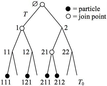
We will obtain upper bounds for these sums over the equivalence class [I] in terms ofpth powers of f summed across certain levels of the tree T.

Figure 1: Particles and join points in the example

To illustrate this, consider a specific case of the binary rooted tree of k = 3 lev-els with n = 4 particles. Starting with the configuration (111,121,211,212) of points of T0 (with the usual coding of vertices of the binary tree) the join points are at ∅,1

(g(111), g(121), g(211), g(212)) obtainable under an automorphismg of the rooted treeT. Assign each free vertexi∈T0 a positive weightµ(i). For each vertex j∈T write µ(j) for

the total weight of the free vertices below j, so, for example, µ(21) = µ(211) +µ(212). In this special case, our main inequality becomes, for any non-negative functionf on the vertices ofT and for allp1, p2, p3 >2 satisfying _p1

1 +

1

p2 +

1

p3 = 1, X

(i1,i2,i3,i4)∈[I]

µ(i1)µ(i2)µ(i3)µ(i4)F(i1,i2,i3,i4) (1.2)

≤ 8·81/p1 _·41/p2 _·21/p3 _{f(∅)µ(∅)}1+p11/p1

× f(1)p2_µ(1)1+p2 _+f(2)p2_µ(2)1+p21/p2

× f(11)p3_µ(11)1+p3 _+f(12)p3_µ(12)1+p3

+f(21)p3_µ(21)1+p3 _+f(22)p3_µ(22)1+p31/p3_{. (1.3)}

The sum (1.2) has 64 terms, each a product over 3 join points, one at each level 0, 1 and 2. The bound (1.3) is a product of weighted pith power sums of f across each of the 3

levels of the tree at which the join points occur. A check shows that equality holds if the weights µ(i) are equal for all i ∈ T0 and f is constant across each level, that is if

f(1) =f(2) andf(11) =f(12) =f(21) =f(22).

We will prove results of this type in a general context by employing induction with respect to automorphisms fixing the join points and incorporating H¨older’s inequality in a natural way.

2

Notation and statement of results

To state the main results we set out some further notation relating to the treeT.

For integers m ≥ 2 and k ≥ 1, we index the vertices of T, the m-ary regular rooted tree ofk+ 1 levels (including the level of the root), by thesymbolic space of words formed from the symbols {1,2, . . . , m}. Thus the vertices of T are given by {(i1, i2, . . . , il) : 0 ≤

l ≤k, 1≤ij ≤ m}, with the root of the tree as the empty word ∅. We often abbreviate

a word by i = (i1, i2, . . . , il) and write |i| = l for its level or generation. The set of free

vertices, that is those iwith |i|=k, is denoted by T0. We write ij to mean that iis a

curtailmentof j, that is i is an initial subword of j. If i,i0 ∈ T then the join i∧i0 is the maximal word such that bothi∧i0 i and i∧i0 i0. With each j ∈T we associate the

cylinderCj ={i∈T0 :ji} comprising those points ofT0 belowj.

We next consider automorphisms of the rooted tree T, regarded as a graph, which induce permutations of the vertices at each level of the tree. For each vertex v∈ T and 1≤n ≤mk _{we write}

Sv(n) =

(i1, . . . ,in) :ij ∈T0, ij v(1≤j ≤n), ij 6=ih(j 6=h) (2.1)

for the set of all orderedn-tuples of distinct elements of T0 that are descendents ofv. Let

Autvbe the group of automorphisms of the rooted treeT that fixv. Define an equivalence

relation∼ onSv(n) by

(i1, . . . ,in)∼(i01, . . . ,i

0

n) if there exists g ∈Autv such thatg(ir) = i0r for all 1≤r≤n;

thus the equivalence classes are the orbits of Sv(n) under Autv. We write [I]v for the

equivalence class containingI = (i1, . . . ,in). For notational simplicity, we often omit the

subscript when v=∅, so that S(n) =S∅(n) and [I] = [I]∅.

We require some terminology relating to the joins of subsets ofT0. LetI = (i1, . . . ,in)∈

Sv(n). Thejoin setofI, denoted byV(I) = V(i1, . . . ,in), is the set of vertices{j1, . . . ,jn−1} ⊂

T consisting of the join points ii ∧ij for all 1 ≤ i < j ≤ n, with w ∈ V(I) occurring

with multiplicity r if there are (r+ 1) distinct indices 1 ≤i1 < . . . < ir+1 ≤ n such that

iis∧iit =wfor alls6=t. Note that the join set ofn points always consists ofn−1 points

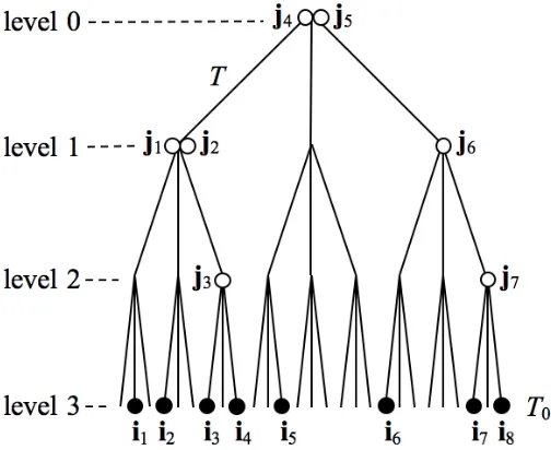
counting by multiplicity. Moreover, if T is a binary tree, so m = 2, all join points have multiplicity 1.

Figure 2: A 3-ary tree with 8 particles and 7 join points, 2 of which have multiplicity 2

The set of join levels L(I) of I ∈ Sv(n) is {|j1|, . . . ,|jn−1| : ji ∈

V

(I)} with levels repeated according to multiplicity. Notice that ifI ∼I0 thenL(I) =L(I0) =:L([I]v), i.e.

the set of levels is constant across each equivalence class [I]v of Sv(n).

For a levelLofT we will, by slight abuse of notation, writej∈Lto mean that|j|=L, so we think of a vertexj ‘belonging’ to a level of the tree.

We now assign a weight µ(i) ≥ 0 to each i ∈ T0. Then the weight of each cylinder

is defined to be the sum of the weights of the points in the cylinder, that is µ(Cj) =

P

i∈T0,jiµ(i) for each j∈T.

Next we assign a positive value f(j) to each vertex j of T, that is f :T →_R+_{. Then}

for each I ∈ S(n) we take the product of these values over the join points of I. Thus if n≥2 we define F :S(n)→_R+ _by

F(i1, . . . ,in) =f(j1)f(j2)· · ·f(jn−1), (2.3)

where I = (i1, . . . ,in) ∈ S(n) has join set

V

(i1, . . . ,in) = {j1, . . . ,jn−1}. For I = (i1) ∈

S(1) we make the trivial assignmentF(i1) = 1. Note that ifjis a join point of multiplicity

Theorem 2.1 Let T be the rooted m-ary tree of k levels. Let 2≤n ≤mk_{. Let I ∈S(n)}

have join points at levelsL1, . . . , Ln−1 and let p1, . . . , pn−1 >0 satisfy Pn

−1

i=1 1

pi = 1. Then

X

(i1,...,in)∈[I]

µ(i1)· · ·µ(in)F(i1, . . . ,in)≤K n−1

Y

i=1

X

j∈Li

f(j)pi_µ(C

j)1+pi

1/pi

, (2.4)

where K does not depend onf or µ.

The value of the constant K will be discussed in Section 4. We obtain the following estimate, though this is not in general optimal.

Corollary 2.2 We may take K =

j

Y

i=1

(m−1)! (m−ri−1)!

≤ (m− 1)n−1 in (2.4), where the

product is over the distinct join points which have multiplicities r1, . . . , rj. In particular,

for a binary tree, where m= 2, we can take K = 1.

For a binary tree we can, under certain conditions, improve on this to obtain the best possible value ofK.

Corollary 2.3 Let T be the rooted binary tree of k levels. Let 2 ≤ n ≤ 2k_{. Let I ∈}

S(n) have join points {j1, . . . ,jn−1} at levels L1, . . . , Ln−1 and let p1, . . . , pn−1 >0 satisfy

Pn−1

i=1 1

pi = 1. Suppose also that the following condition is satisfied:

If the join points of I are ordered so that j1 is the ‘top’ join point (i.e. j1 ji for all

i) and {j2, . . . ,jm} and {jm+1, . . . ,jn} are the join points below the left and right edges

abutting j1 respectively, then

m

X

i=2

1 pi

≤ 1

2 and

n

X

i=m+1

1 pi

≤ 1

2. (2.5)

Then

X

(i1,...,in)∈[I]

µ(i1)· · ·µ(in)F(i1, . . . ,in)≤

1 2n−1

n−1

Y

i=1

X

j∈Li

f(j)pi_µ(C

j)1+pi

1/pi

, (2.6)

with equality if µ(i) is constant for all i ∈ T0 and, for each level Li, f(j) is constant for

all j∈Li.

3

Proof of Theorem 2.1

In the proof of Lemma 3.1 we will refer to the numbers K(m;a1, . . . , am), defined as

follows form ≥1 and ai ≥0. With Sm as the symmetric group of all permutations σ of

(1,2, . . . , m), K(m;a1, . . . , am) is the least number such that

X

σ∈Sm

xa1

σ(1)x

a2

σ(2)· · ·x

am

σ(m) ≤K(m;a1, . . . , am)(x1+· · ·+xm)a1+···+am (3.1)

for allxi ≥0, where we make the consistent convention that 00 = 1. It is easy to see that

K(m;a1, . . . , am)≤m! ; we will discuss the value of K in more detail in Section 4.

Lemma 3.1 Let T be the rooted m-ary tree of k levels. Let v ∈T and 1≤ n ≤ mk−|v|_.

Let I ∈ Sv(n) have join points at levels L1, . . . , Ln−1 and let p1, . . . , pn−1 > 0 satisfy

Pn−1

i=1 1

pi = 1. Then

X

(i1,...,in)∈[I]v

µ(i1)· · ·µ(in)F(i1, . . . ,in)≤K n−1

Y

i=1

_X

j∈Li,jv

f(j)pi_µ(C

j)1+pi

1/pi

, (3.2)

where K does not depend onf or µ.

Proof. We proceed by strong induction. We take the inductive hypothesisP(n) forn ∈_N

to be as follows.

P(n) (n ≥ 1): For all v ∈ T, for all p1, . . . , pn−1 > 0 and 1 ≤ α ≤ ∞ satisfying

Pn−1

i=1 1

pi = 1−

1

α, if I ∈ Sv(n) has join levels L1, . . . , Ln−1, there is a constant K such

that

X

(i1,...,in)∈[I]v

µ(i1)· · ·µ(in)F(i1, . . . ,in)≤Kµ(Cv)1/α

n−1

Y

i=1

_X

j∈Li,jv

f(j)pi_µ(C

j)1+pi

1/pi

,

(3.3) for all µand f.

When n = 1 then α= 1 and we take the empty product to equal 1 in (3.3). The proof falls into several parts.

(a) Verification of P(1). If v∈T and I = (i1)∈Sv(1) then

X

(i1)∈[I]v

µ(i1)F(i1) =

X

i1v

µ(i1) =µ(Cv),

which isP(1) with K = 1, noting thatα = 1.

(b) The inductive step. Assume, for some integer n ≥ 2, that P(l) holds for all 1 ≤l ≤

n−1. We will show that P(n) holds. Let v ∈ T and I = (i1, . . . ,in) ∈ Sv(n) where,

without loss of generality, (i1, . . . ,in) are indexed in lexicographical order. We consider

two cases.

Case(b1). Suppose that v∈T is a join point ofI of multiplicityd−1 (2≤d ≤m). Let v1, . . . ,vd be the vertices of T that are children ofv and are above at least one of the ij,

that is for eachj, |vj| =|v|+ 1 and there is an k such that v vj ik. Then I splits

into d non-empty parts, Ij = (ij1, . . . ,ijnj) for 1 ≤j ≤d, so that i

j

i vj for all i, j, with

nj ≥1 and n1+· · ·+nd =n. Note that the join points of I comprise the join points of

Let p1, . . . , pn−1 > 0 be the exponents associated with the join points of I where

Pn−1

i=1 1

pi = 1−

1

α with 1 < α ≤ ∞. Re-index these exponents so that p j

1, . . . , p

j

nj−1 are

those associated with the join points of Ij for each j and the exponents p01, . . . , p0d−1 are

those associated withv. Let the corresponding join levels ofIj be Λ(Ij) ={Lj1, . . . , L

j nj−1}

for 1≤j ≤d. Define α1, . . . , αd by

nj−1

X

i=1

1

pj_i = 1− 1 αj

<1 (if nj ≥2) or αj = 1 (if nj = 1). (3.4)

Summing overj gives

1 α1

+· · ·+ 1 αd

=d−1 + 1 p0 1

+· · ·+ 1 p0

d−1

+ 1

α =d−1 + 1

β (3.5)

where, for convenience, we write 1/β = 1/p0

1+· · ·+ 1/p0d−1+ 1/α.

Now let (v1, . . . ,vd, . . . ,vm) be the set ofallvertices ofT immediately belowv. LetG

be a subgroup of Autv such that{(g(v1), . . . , g(vm)) :g ∈G}includes every permutation

of (v1, . . . ,vm) exactly once, so thatGhas orderm!. The orbits ofI may be decomposed

as

[I]v={([g(I1)]g(v1), . . . ,[g(Id)]g(vd))}g∈G,

but ifm≥d+ 2 then (m−d)! elementsg ofGwill yield each such decomposition of [I]v.

Then, by definition of F,

(m−d)! X

(i1,...,in)∈[I]v

µ(i1)· · ·µ(in)F(i1, . . . ,in)

=X

g∈G

f(v)d−1

X

(i1

1,...,i1n1)∈[g(I1)]g(v1)

µ(i1₁)· · ·µ(i1_n1)F(i1₁, . . . ,i1_n1)

× · · · ×

X

(id

1,...,idnd)∈[g(Id)]g(v_d)

µ(id₁)· · ·µ(id_n

d)F(i

d

1, . . . ,i

d nd)

≤f(v)d−1X

g∈G

K1µ(Cg(v1))

1/α1

n1−1 Y

i=1

_X

j∈L1

i,jg(v1)

f(j)p1iµ(C

j)1+p

1

i

1/p1i

× · · · ×

Kdµ(Cg(vd))

1/αd

nd−1

Y

i=1

_X

j∈Ld i,jg(vd)

f(j)pdiµ(C

j)1+p

d i

1/pdi

(on applying (3.3) to eachIj in the decomposition ofI, with Kj as the corresponding constant K)

=K1· · ·Kdf(v)d−1

X

g∈G

µ(Cg(v1))

1/α1_{· · ·µ(C}

g(vd))

1/αd

×

n1−1 Y

i=1

_X

j∈L1

i,jg(v1)

f(j)p1iµ(C

j)1+p

1

i

1/p1i

× · · · ×

nd−1

Y

i=1

_X

j∈Ld i,jg(vd)

f(j)pdiµ(C

j)1+p

d i

1/pdi

≤K1· · ·Kdf(v)d−1

X

g∈G

µ(Cg(v1))

β/α1_{· · ·µ(C}

g(vd))

β/αd

×

n1−1 Y

i=1

X

g∈G

X

j∈L1

i,jg(v1)

f(j)p1iµ(C

j)1+p

1

i

1/p1_i

× · · · ×

nd−1

Y

i=1

X

g∈G

X

j∈Ld i,jg(vd)

f(j)pdiµ(C

j)1+p

d i

1/pd_i

(using H¨older’s inequality, noting that _β1 +Pd

j=1

Pnj−1

i=1 1

pj_i = 1)

≤K1· · ·Kdf(v)d−1K(m;β/α1, . . . , β/αd,0, . . . ,0)1/β µ(Cv1) +· · ·+µ(Cvm)

1/α1+···+1/αd

×

n1−1 Y

i=1

(m−1)!X

j∈L1

i,jv

f(j)p1i_µ(C

j)1+p

1

i

1/p1_i

× · · · ×

nd−1

Y

i=1

(m−1)! X

j∈Ld i,jv

f(j)pdi_µ(C

j)1+p

d i

1/pd_i

(whereK(m;· · ·) is given by (3.1))

=K0f(v)d−1µ(Cv)d−1+1/p

0

1+···+1/p0d−1+1/α

Y

1≤j≤d,1≤i≤nj−1

X

j∈Lj_i,jv

f(j)pjiµ(C

j)1+p

j i

1/pji

(whereK0 =K1· · ·KdK(m;β/α1, . . . , β/αd,0, . . . ,0)1/β(m−1)!1−1/β and using (3.5))

(3.6)

=K0µ(Cv)1/α f(v)p

0 1µ(C

v)1+p

0 11/p

0

1_{· · · f(v)}p0_d−1µ(C

v)1+p

0

d−11/p 0

d−1

× Y

1≤j≤d,1≤i≤nj−1

_X

j∈Li,jv

f(j)pjiµ(C

j)1+p

j i

1/pj_i

=K0µ(Cv)1/α

Y

0≤j≤d,1≤i≤nj−1

_X

j∈Li,jv

f(j)pji_µ(C

j)1+p

j i

1/pj_i

(on incorporating the terms involving pj₀ as single terms in the product)

=K0µ(Cv)1/α

n−1

Y

i=1

_X

j∈Li,jv

f(j)pi_µ(C

j)1+pi

1/pi

.

ThusP(n) holds withK =K0/(m−d)!.

Case(b2). Now suppose thatv is not a join point of I. As before let p1, . . . , pn−1 >0 be

the exponents associated with the join points ofI wherePn−1

i=1 1

pi = 1−

1

α with 1< α≤ ∞.

Let w be the first join point of I below v, so that i1, . . . ,in w v, with n ≥ 2. Let

v1, . . . ,vr be the vertices ofT such thatvj vand |vj|=|w|, and letgj ∈Autv be such

that gj(w) = vj. We may decompose the orbits ofI as

[I]v ={[gj(I)]vj}

r j=1.

Applying case (b1) to [gj(I)]vj for 1 ≤j ≤r, and lettingK be the corresponding constant

given by (3.3), which will be the same for eachj, we obtain

X

(i1,...,in)∈[I]v

µ(i1)· · ·µ(in)F(i1, . . . ,in)

=

r

X

j=1

X

(i1,...,in)∈[gj(I)]v_j

µ(i1)· · ·µ(in)F(i1, . . . ,in)

≤

r

X

j=1

Kµ(Cvj)

1/α n−1

Y

i=1

_X

j∈Li,jvj

f(j)pi_µ(C

j)1+pi

≤K

r

X

j=1

µ(Cvj)

1/αn_Y−1

i=1

_Xr

j=1

X

j∈Li,jvj

f(j)pi_µ(C

j)1+pi

1/pi

=Kµ(Cv)1/α

n−1

Y

i=1

_X

j∈Li,jv

f(j)pi_µ(C

j)1+pi

1/pi

using H¨older’s inequality, to get (3.3) in this case.

Thus by induction P(n) holds for all n ≥ 1, and the Lemma follows if n > 1 taking α=∞. 2

Proof of Theorem 2.1The theorem is immediate on setting v=∅ in (3.3). 2

4

Value of the constant

K

The constantKthat occurs in (2.4) arises from a product of termsK(m;β/α1, . . . , β/αd,0, . . . ,0)

that are incorporated at (3.6) at each step of the induction. Thus to estimate K we first need to boundK(m;a1, . . . , am).

Lemma 4.1 Let m≥1 and let ai ≥0 for i= 1,2, . . . , m, with 0< a1+a2+· · ·+am =

s. Let Sm be the symmetric group of all permutations σ of (1,2, . . . , m). Recall that

K(m;a1, . . . , am) is the least number such that

X

σ∈Sm

xa1

σ(1)x

a2

σ(2)· · ·x

am

σ(m)≤K(m;a1, . . . , am)(x1+x2+· · ·+xm)

s

(4.1)

for all xi ≥0, with the convention that 00 = 1.

(i) If 0< s≤1 then

K(m;a1, . . . , am) =m!m−s.

(ii) If 1≤s then

m!m−s ≤K(m;a1, . . . , am)≤(m−1)!.

(iii) If 1≤s and ai ≥(s−1)/m for all i= 1, . . . , m then

K(m;a1, . . . , am) =m!m−s.

(iv) For m= 2, if (a1−a2)2 ≤a1+a2 then

K(2;a1, a2) = 21−s = 21−a1−a2.

With the values given in (i), (iii) and (iv) there is equality in (4.1) if and only if the xi

are all equal.

Proof. It is enough to prove (4.1) with the xi >0 and take the limit of the inequality for

any xi = 0. Modifying the exponents to sum to 1 and then using Muirhead’s inequality

(see [4, 5]) gives

1 m!

X

σ∈Sm

xa1

σ(1)x

a2

σ(2)· · ·x

am

σ(n) =

1 m!

X

σ∈Sm

(xs_σ(1))a1/s_(xs

σ(2))

a2/s_{· · ·(x}s

σ(m))

≤ 1

m(x

s

1+x

s

2+· · ·+x

s m).

Then (i) follows directly on applying the generalized mean inequality and (ii) follows using Minkowski’s inequality. Note that in case (ii), settingK =m!m−sin (4.1) we get equality when the xi are all equal but the inequality may fail with this K for other xi. For (iii)

we have

1 m!

X

σ∈Sm

xa1

σ(1)x

a2

σ(2)· · ·x

am

σ(n) =

1 m!

X

σ∈Sm

xa1−(s−1)/m

σ(1) · · ·x

am−(s−1)/m

σ(n) xσ(1)xσ(2)· · ·xσ(m)

(s−1)/m

≤ 1

m(x1+x2+· · ·+xm) (x1+x2+· · ·+xm)/m

s−1

using Muirhead’s inequality and the geometric-arithmetic mean inequality. For (iv) we first claim that for all r, q ≥0 such that (r−q)2 _≤r+q

cosh(r−q)θ

(coshθ)r+q <1 for all 06=θ ∈R. (4.2)

To see this, assume, without loss of generality, that 0≤q < r. Differentiating and using the addition formula for hyperbolic functions gives

d dθ

cosh(r−q)θ (coshθ)r+q

= rsinh (r−q−1)θ

−qsinh (r−q+ 1)θ

(coshθ)r+q_coshθ . (4.3)

Note that

r(r−q−1)−q(r−q+ 1) = (r−q)2−(r+q)≤0

from our assumption. Since (r−q−1)2 _{< (r−q+ 1)}2 _{and q(r−q+ 1) ≥ 0 it follows}

inductively that

r(r−q−1)2k+1−q(r−q+ 1)2k+1 <0 (4.4) for all integers k ≥ 1. But the left-hand expression in (4.4) is just the coefficient of θ2k+1/(2k+ 1)! in the power series expansion of the numerator of the quotient in (4.3). Thus the derivative (4.3) is strictly positive forθ <0 and strictly negative forθ >0, from which (4.2) follows.

Ifx1 =λx2 where λ >0 and settingλ1/2 = eθ,

xr

1x

q

2+xr2x

q

1

(x1+x2)r+q

= λ

(r−q)/2_+λ(q−r)/2

(λ1/2 _+λ−1/2₎r+q =

e(r−q)θ_{+ e}−(r−q)θ

(eθ_{+ e}−θ₎r+q = 2

1−r−qcosh(r−q)θ

(coshθ)r+q ≤2

1−r−q

by (4.2), with equality if and only ifx1 =x2. Taking r =a1 and q=a2 gives (iv). 2

Note that case (iv) of inequality (4.1) when m= 2 is related to Muirhead means and Schur convexity, which has a substantial literature, see [1, 4]. Some related inequalities are obtained in [1, 6] but we were unable to find the particular inequality that we required. Note also in relation to case (iv) that if (a1 −a2)2 > a1 +a2 then the maximum of

P

σ∈S2x

a1

σ(1)x

a2

σ(2)

(x1+x2)a1+a2 does not necessarily occur when x1 = x2, in which case

K(2;a1, a2)>21−a1−a2.

Proof of Corollary 2.2 Each time the induction step is applied at a join point with mul-tiplicityd−1 the constant gets multiplied at (3.6) by

≤(m−1)!1/β(m−1)!1−1/β(m−d)!−1 = (m−1)!(m−d)!−1

using Lemma 4.1(ii). The induction step is applied once at each join point, so the estimate forK follows. Noting that (m−1)!/(m−ri−1)! ≤(m−1)ri for eachiandPj_i=1ri =n−1

gives the stated inequality. 2

In general the value ofK stated in Corollary 2.2 will not be optimal which in the case of a binary tree gives K = 1. However, provided that the exponents pi are reasonably

well distributed in the manner stated precisely in Corollary 2.3, we can reduce this to K = 2−(n−1).

Proof of Corollary 2.3 For a binary tree, m = 2, all the join points are of multiplicity 1, and the inductive step is appliedn−1 times. Thus the corollary will follow if we can show that the multiplier incorporated at (3.6) each time the inductive step is used satisfies

K(2;β/α1, β/α2)1/β ≤2−1.

Note that (2.5) implies that at each stage of the induction 1/α1,1/α2 ≥ 1₂ each time

(3.4) is used. In particular (1/α1 −1/4)(1/α2−1/4)≥1/16 which rearranges to

1 α1

+ 1 α2

≤ 4

α1α2

. (4.5)

Then

1 α1

− 1

α2

2

= 1

α2 1

+ 1 α2

2

− 2

α1α2

≤

1 α2

1

+ 1 α2

2

+ 2

α1α2

−

1 α1

+ 1 α2

=

1 α1

+ 1 α2

1 α1

+ 1 α2

−1

=

1 α1

+ 1 α2

1 β

using (3.5), giving

β α1

− β

α2

2

≤ β

α1

+ β α2

.

Thus Lemma 4.1 (iv) gives

K(2;β/α1, β/α2)1/β ≤2(1−β/α1−β/α2)/β = 2−1

as required. 2

Finally note that conditions for equality are not in general easy to specify. This requires equality at each step of the induction when H¨older’s inequality and (4.1) are applied. There will be equality in Theorem 2.1 if µ(i) is constant for all i ∈ T0 and

f(j) is constant for all j ∈ Li for each level Li provided that we have the optimal value

of K. This we can do under the conditions of Corollary 2.3. However, as the value of K(m;a1, . . . , am) for Lemma 4.1 case (iii) seems to be unknown when m ≥3 and s > 1,

5

Acknowledgement

The author is most grateful to the referee for a number of helpful suggestions.

References

[1] Yu-Ming Chu and Wei-Feng Xia, Necessary and sufficient conditions for the Schur harmonic convexity of the generalized Muirhead mean, Proc. A. Razmadze Math. Inst. 152 (2010) 19–27.

[2] K.J. Falconer, Generalized dimensions of measures on almost self-affine sets, Nonlinearity 23 (2010) 1047–1069.

[3] K.J. Falconer and Yimin Xiao, Generalized dimensions of images of measures under Gaussian processes, Adv. Math. 252 (2014) 492–517.

[4] D.J.H. Garling, Inequalities: a Journey into Linear Analysis, Cambridge Univer-sity Press (2007).

[5] G.H. Hardy, J.E. Littlewood and G. P´olya, Inequalities, Cambridge University Press, Pbk. Ed. (1988).