doi:10.4236/jbise.2010.33043 Published Online March 2010 (http://www.SciRP.org/journal/jbise/).
A mixture model based approach for estimating the FDR in
replicated microarray data
Shuo Jiao, Shun-Pu Zhang
Department of Statistics University of Nebraska Lincoln, NE, USA. Email: [email protected]
Received5 November 2009; revised 27 November 2009; accepted 3 December 2009.
ABSTRACT
One of the mostly used methods for estimating the false discovery rate (FDR) is the permutation based method. The permutation based method has the well-known granularity problem due to the discrete nature of the permuted null scores. The granularity problem may produce very unstable FDR estimates. Such instability may cause scientists to over- or under-estimate the number of false positives among the genes declared as significant, and hence result in inaccurate interpretation of biological data. In this paper, we propose a new model based method as an improvement of the permutation based FDR estimation method of SAM [1] The new method uses the t-mixture model which can model the microarray data better than the currently used normal mixture model. We will show that our proposed method provides more accurate FDR estimates than the permutation based method and is free of the problems of the permutation based FDR estimators. Finally, the proposed method is evaluated using extensive simulation and real microarray data.
Keywords:FDR; T-Mixture Model; Microarray; Genes
1. INTRODUCTION
Genome-wide expression data generated from the mi-croarray experiments are widely used to uncover the functional roles of different genes, and how these genes interact with each other. A key step to achieve this is to identify the differentially expressed (DE) genes under different experimental conditions. Such information can be used to identify disease biomarkers that may be im-portant in the diagnoses of different types of diseases. Earlier statistical approaches for detecting DE genes focused mostly on parametric methods which are easily subject to model misspecification problems. Some of the well-known parametric methods for detecting DE genes include the two sample t-test [2], the analysis of variance approach [3], a regression approach [4], the regularized
t-statistic method (Bayes-t test) [5,6]), the semi- parametric hierarchical mixture method [7], and the pa-rametric EB method [8]. Recently, the availability of replicated microarrays has made it possible to use the nonparametric methods to detect the DE genes. The nonparametric methods require much less stringent dis-tributional assumptions, and thus can provide more robust results than the parametric methods. Some of the well-known nonparametric methods for analyzing mi- croarrays include the Significance Analysis of Mi-croar-ray (SAM) of [1], the nonparametric EB method [9,10], the non-parametric t-test with adjusted p-value [11], the Wilcoxon Rank Sum test [12], samroc [13] and the normal mixture model method (MMM) of [14].
In this paper, we will focus our attention on SAM, one of the most popular methods in microarray data analysis. SAM indentifies DE genes by computing a modified
t-statistic as the test score of a gene and finding the genes with test scores exceeding an adjustable threshold. The false discovery rate (FDR) was then estimated by a permutation based method. More specifically, the num-ber of false positive (FP) genes among the significant genes is estimated as the median of the numbers of scores exceeding the cutoffs in each permuted set of null scores.
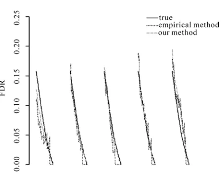
Since the permutation based approach estimates the FDR by counting the number of FP genes exceeding some cutoffs, we will call it the empirical method in this paper. Due to its nature, there are two drawbacks with the empirical method: 1) the granularity problem – the FDR estimates based on the counted number of FP genes tend to be unstable when the actual number of FP genes is small; 2) the zero FDR problem – the estimated FDR may be zero when the range of the permuted null scores is smaller than that of test scores and when the cutoffs are more extreme than the endpoints of permuted null scores. These two drawbacks are illustrated in the Fig-ures 1, 2 and 3.
Figure 1. Comparison of true FDR, the empirical FDR estimator
[image:2.595.312.530.78.275.2]FDR and the model based FDR estimator FDR1 for two sample microarray data. 5 replicates are listed. Total number of significant genes is decreasing from 100 to 1 (left to right) for each replicate.
Figure 2. Comparison of true FDR, the empirical FDR estimator
FDR and the model based FDR estimator FDR1 for two sample microarray data. 5 replicates are listed. Total number of significant genes is decreasing from 150 to 1 (left to right) for each replicate.
FDR estimation method: The granularity and the zero FDR problems. The performance of our method is as-sessed by applying them to simulated and real microar-ray data.
2. METHODS
2.1. SAM
2.1.1. SAM algorithm
Let Yij be the expression levels of genes i under array j
Figure 3. Comparison of the empirical FDR estimator FDR
and the model based FDR estimator FDR1 for Leukemia microarray data.
(i=1,…,n; j=1,… , +1,…, ), and the first and last arrays are obtained under two conditions. We need to test if gene i has differential ex-pressions under the two conditions.
1 j
2 j
1
j j1 j2 J
1 j
In SAM, the test statistic is defined as:
(1) (2)
2
1 2
(1 / 1 / ) i i i
i
Y Y Z
j j s
0
s
,
where , are the sample means under two
con-ditions;
(1)
i
Y
2
i
(2)
i
Y
s is the pooled sample variance; s0 is the
fudge factor. The null score is then computed by applying the test statistic to the b-th set of permuted data.
b i
z
In the SAM manual [15], the following algorithm is given to detect DE genes. First, all genes are ranked by the magnitude of their test scores Zi so that Z(1) is
the largest test score and Z( )i is the i-th largest test score. For the b-th set of null scores, the same procedure is applied so that is the i-th largest null score in the
b-th set of null scores. The expected relative difference is then defined as . After that, a scatter
plot of
( )
b i
z
( ) ( ) 1
/
z
B E b
i i b
z
B( )i
Z vs. ( )
E i
z is plotted. In the scatter plot, some
points are displaced from the Z( )i = ( )E i
z line with a
distance greater than , a pre-specified threshold. In [16], the author pointed out that the estimated total number of significant (TS) genes and FP genes obtained using the SAM algorithm can be written as:
( ) ( )
#{ ; i U or i L}
[image:2.595.58.277.349.510.2]S. Jiao et al. / J. Biomedical Science and Engineering 3 (2010) 317-321
( ) ( ) 1
#{ ; or z } / B
b b i U i L b
FP i z
B, (2)where U and L are the upper and lower cutoffs decided by the pre-specified threshold . For simplic-ity, we only consider symmetric cutoffs (| | |
|
U L
) in this paper though extensions to asymmetric cutoffs are straightforward. Under symmetric cutoffs, (1) and (2) can be written as:
( )
( ) #{ ;| i | }
TS i Z (3)
( ) 1
( ) #{ ;| | } /
B b
i b
FP i z
B (4)2.1.2. Empirical FDR Estimator of SAM
Given a gene-specific significance level (0, 1] and assume that we have obtained the p-values for all the genes under consideration, the FDR of [17] is defined as:
( ) [
( )
N
FDR E
TS ]
, (5)
where N( ) is the number of genes among the EE genes whose p-values are less than or equal to , and
(
TS) is the number of genes among all the genes whose p-values are less than or equal to (or it is the total number of significant genes). Instead of controlling gene-specific significance level , SAM usually con-trols the total number of significant genes by setting a corresponding cutoff , hence (5) can be re-written as:
( ) [
( )
N
FDR E
TS ]
, (6)
where N( ) is the number of EE genes with absolute value of Zi greater than , and TS( ) is the total number of genes with absolute value of Zi greater than .
It was shown in [18] that the FDR can be approxi-mated by
[ ( )] [ ( )]
E N FDR
E TS
. (7)
Since N( ) is the number of false positive among the EE genes, denote the proportion of EE genes by 0,
(7) becomes
0 [ ( )] [ ( )]
E FP FDR
E TS
, (8)
where FP( ) is the number of FP if all the genes are
EE. FP( ) and TS( ) can be estimated by FP( )
and TS( ) in (3) and (4), respectively. As a result, the empirical FDR estimator of SAM is
0 ˆ ( )
( )
FP FDR
TS
, (9)
As mentioned before, this empirical FDR estimator of SAM has the granularity problem and the zero FDR problem. In the following sections, we solve these prob-lems by proposing a model based FDR estimation method.
2.2. The T-mixture Model (TMM) Based FDR Eestimation Approach
Let f be the probability density of the test score Zi
and be the density of null score . In TMM, it is assumed that the data are from several components with distinguished t-distributions. In other words, both and are considered to be a mixture of the t-distribu-
0 f
0 f
b i
z
f
tions with probability density function:
1
( ; ) ( ; , , )
g
g i i i i
h z z i
, (10)where ( ;z i,i, )i denotes the t-distribution density function with mean i, variance , and degrees of freedom
i
i
. The coefficients i are the mixing pro-portions and g is the number of components, which can be selected adaptively. g denotes all the unknown
parameters (i , i, i, i) | in (5). The mixture model is fitted by maximum likelihood using an expectation conditional maximization (ECM) algorithm [19]. The final model is selected based on Bayesian In-formation Criterion (BIC). More details on how to fit the TMM to microarray data can be found in [20]. It was reported in their paper that not only does the TMM ap-proach provide more accurate estimates of the densities, but also it enjoys computational efficiency since it was demonstrated in [20] that one only needs to use one set of permuted null scores to fit the t-mixture model. More specifically, instead of using all ’s (size=n*B) to fit the t-mixture model, a random sample with size n can be drawn from and used as the null statistics.
1,.
i
b i
..g
z
1 1
B n b i b i
z
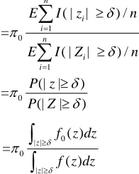
Since the test statistic Zi and the null statistic (because only one set of null score is used now, we will denote the null statistic as instead of ) have the densities
i
z
i
z zib
f and f0, respectively, it is easy to see from
(8) that
0
[ ( ) / ]
[ ( ) / ]
E FP n
FDR
E TS n
1 0
1
0
( | | ) / =
( | | ) /
(| | ) =
(| | ) n
i i
n
i i
E I z n
E I Z n
P z P Z
0 | | 0
| | ( ) =
( )
z
z
f z dz
f z dz
(11) where is chosen such that a given number of sig-nificant genes is detected. Equation (11) can be viewed as the model based formula of FDR.Assume that we have available the estimators fˆ and
0
f of and from the TMM, respectively, then the corresponding model based FDR estimator for (11) is
f f0
0 | | 1 0
| | ( ) FDR =
( )
z
z
f z dz
f z dz
, (12) The model based FDR estimator (12) has the follow-ing advantages compared to the empirical FDR estimator of SAM:1) It does not have the granularity problem of the em-pirical FDR estimator (9);
2) It provides non-zero FDR estimate for any
, while (9) only provides non-zero FDR when cutoffs are within the two endpoints of the range of the permuted null scores;3) Unlike (9), the numerator and the denominator of (12) are not subject to the sampling variability.
3. RESULTS
3.1. Simulated Data
In the simulation, replicates and n = 5,000 genes are generated while 200 of them are assumed to be differentially expressed. For the DE genes, the data un-der condition 1 are generated from N(2,1) and the data under condition 2 are generated from N(0,1). The EE genes are generated from N(0,1)regardless of the condi-tions. For the generated data, we calculate the true FDR and estimated FDR for a grid of total number of signifi-cant genes ranging from 100 to 1 (in decreasing order). This procedure is repeated for five times. Figure 1 shows comparisons of true FDR, empirical FDR estima-tor
1 2 4
j j
FDR defined by (9), and the model based FDR
estimator FDR1 defined by (12).
As we can see, the instability of empirical FDR in-creases significantly as it dein-creases to 0, which shows its granularity problem. Another fact worth noticing is that
FDR tends go to zero faster than the true FDR, which is the zero FDR problem. It can be seen that the true FDR strictly decreases as the total number of significant genes decreases. However, the empirical FDR does not show this characteristic. In contrast, FDR1 captures
the decreasing trend very well and does not have the erratic jumps of FDR. To check how well these two FDR estimators approximate the true FDR, we calculate the mean squared error for both of them. MSE for FDR
is 0.00045 and MSE for FDR1
2
) i i
is 0.00021, which shows that our method outperforms the empirical method.
Next, we compare the performances of the two meth-ods when the two populations for the DE and EE genes are not so well separated. For this purpose, we conduct an-other simulation which tries to mimic the real data. The expression levels for the EE genes under the two conditions are generated from N( 1, and 2
1
( i , i )
N with
1 2
i i
. The
expres-sion levels for the DE genes are generated similarly as the EE genes, except that
~N(0, 2) i2
~ Gamma(4, 2)
1
i
and i2 are generated
[image:4.595.133.231.85.207.2]from separately. In this case, the grid of total number of significant genes ranges from 150 to 1 (in decreasing order). Comparison results are displayed in Figure 2.
(0
N , 2)
It is seen from Figure 2 that FDR isvery unstable and approximates true FDR poorly, which makes the estimates highly inaccurate. On the other hand, FDR1
has a much smoother curve than FDR and seems to be able to capture the decreasing trend of the true FDR very well. In addition, the fact that MSE for FDR is 0.025 and for FDR1 is 0.015 shows that our method gives a
significantly better fit to the true FDR.
3.2. Real Data
The Leukemia data of [21] is one of the most studied gene expression data sets. This data set includes 27 acute lymphoblastic leukemia (ALL) samples and 11 acute myeloid leukemia (AML) samples for 7129 genes. In Figure 3, we estimate the FDRs for different number of significant genes using both our proposed model based FDR estimator and the empirical FDR estimator. As we expect, the model based FDR estimator gives a more stable estimate.
4. DISCUSSION
S. Jiao et al. / J. Biomedical Science and Engineering 3 (2010) 317-321
empirical method. The results also show that our esti-mator provides more stable and accurate estimates of the FDR. The advantage of our method is more evident in the case when DE genes are not well separated with EE genes and the variances of expression levels for every gene are different. This is due to the fact that the permu-tation FDR estimator is more easily affected by the sam-pling variability.
REFERENCES
[1] Tusher, V.G., Tibshirani, R. and Chu, G. (2001) Signifi-cant analysis of microarrays applied to the ionizing ra-diation response. PNAS, 98, 5116-5121.
[2] Long, A. D., Mangalam, H. J., Chan, B. Y. P., Tolleri, L., Hatfield, W. G. and Baldi, P. (2001) Improved statistical inference from DNA microarray data using analysis of variance and a Bayesian statistical frame work, 276, 19937-19944.
[3] Kerr, M.K., Martin, M. and Churchill, G. (2000) Analysis of variance for gene expression microarray data, Journal of Computational Biology, 7, 819-837.
[4] Thomas, J.G., Olson, J.M., Tapscott, S.J. and Zhao, L. P. (2001) An efficient and robust statistical modelling ap-proach to discover differentially expressed genes using genomic expression profiles. Genome Research, 11, 1227-1236.
[5] Baldi, P. L. and Long, A. D. (2001) A Bayesian frame-work for the analysis of microarray expression data: Regularized t-test and statistical inference of gene changes. Bioinformatics, 17, 509-519.
[6] Kendziorski, C. M., Newton, M. A., Lan, H. And Gould, M. N. (2003) On parametric empirical Bayes methods for comparing multiple groups using replicated gene expres-sion profiles. Statistics in Medicine, 22, 819-837. [7] Newton, M., Noueiry, A., Ahlquist, P., Sarkar, D. (2004)
Detecting differential gene expression with a semi-parametric hierarchical mixture method. Biostatistics,
5(2), 155-176.
[8] Smyth, G. K. (2004) Linear models and empirical Bayes methods for assessing differential expression in microar-ray experiments. Statistical Applications in Genetics and Molecular Biology, 3(1).
[9] Efron, B., Tibshirani R., Storey, J. D., Tusher, V. (2001) Empirical Bayes analysis of a microarray experiment.,
Journal of the American Statistical Association, 96, 1151-1160.
[10] Efron, B., Tibshirani, R., Gross, V. and Chu, G. (2000) Microarrays and their use in a comparative experiment, Technical report, Statistics Department, Standard Uni-versity.
[11] Dudoit, S., Yang, H. Y., Callow, J. M. and Speed, P. T. (2002) Statistical methods for identifying differentially expressed genes in replicated cDNA microarray experi-ments. Statistica Sinica, 111-139.
[12] Troyanskaya, O. G., Garber, M. E., Brown, P. O., Bot-stein, D. and Altman, R. B. (2002) Nonparametric meth-ods for identifying differentially expressed genes in mi-croarray data. Bioinformatics, 18, 1454-1461.
[13] Broberg, P. (2003) Ranking genes with respect to differ-ential expression, Genome Biology, 4, R41.
[14] Pan, W., Lin, J. and Le, C. (2003) A mixture model ap-proach to detecting differentially expressed genes with microarray data. Functional & integrative genomics, 3, 117-124.
[15] Chu, G., Narasimhan, B., Tibshirani, R. and Tusher, V. SAM “significance analysis” of microarrays-users guide and technical document, http://www-stat.stanford.edu/~tibs/ SAM/sam.pdf.
[16] Zhang, S. (2007) A comprehensive evaluation of SAM, the SAM R-package and a simple modification to im-prove its performance, BMC Bioinformatics, 8, 230. [17] Benjamini, Y. and Hochberg, Y. (1995) Controlling the
false discovery rate: a practical and powerful approach to multiple testing. Journal of the Royal Statistical Society,
57, 289-300.
[18] Storey, J.D. and Tibshirani, R. (2003) Statistical signifi-cance for genomewide studies. PNAS, 100, 9440-9445. [19] Liu, C. and Rubin, D. (1995) ML estimation of the t
dis-tribution using EM and its extensions ECM and ECME.
Statistica Sinica, 5, 19-39.
[20] Jiao, S. and Zhang, S. (2008) The t-mixture model ap-proach for detecting differentially expressed genes in microarrays. Functional & Integrative Genomics, 8, 181-186.