Optimal Climate Change Policies When Governments
Cannot Commit
1Alistair Ulph
2and
David Ulph
3Abstract
We analyse the optimal design of climate change policies when a government wants to encourage the private sector to undertake significant immediate investment in developing cleaner technologies, but the relevant carbon taxes (or other environmental policies) that would incentivise such investment by firms will be set in the future. We assume that the current government cannot commit to long-term carbon taxes, and so both it and the private sector face the possibility that the government in power in the future may give different (relative) weight to environmental damage costs. We show that this lack of commitment has a significant asymmetric effect: it increases the social benefits of the current government to have the investment undertaken, but reduces the private benefit to the private sector to invest. Consequently the current government may need to use additional policy instruments – such as R&D subsidies – to stimulate the required investment.
JEL Nos: H23, Q54, Q55, Q58
Keywords: Climate Change; Emissions Taxes; Impact on R&D; Timing and Commitment
1 Earlier versions of this paper have been presented to the World Congress of Environmental and Resource Economists, Montreal, 2010 and Towards Global Agreements on Environmental Protection and
Sustainability, Exeter 2011 as well as to workshops at ZEW Mannheim, SCI Manchester, Birmingham and St. Andrews. We are grateful to participants at these events, two anonymous referees, Michael Finus, Partha Dasgupta and Nick Stern for comments. The usual disclaimer applies.
2
Associate Vice-President and Executive Director of Sustainable Consumption Institute: Contact details: Sustainable Consumption Institute, The University of Manchester, Manchester M13 9PL, UK. E-Mail: [email protected]
3
1. Introduction
It is widely recognized (e.g. Stern (2007)) that climate change involves two types of externality: reflecting the global nature of the problem there is an intra-temporal externality whereby countries both affect and are affected by the actions of firms and consumers in all other countries; and there is an inter-temporal externality whereby emissions created by one generation cause damage to many future generations. In this paper we focus exclusively on the inter-temporal externality, so in what follows we assume that there is just a single country that both generates and suffers from climate change.
It is also widely recognized (again, see, for example, Stern (2007)) that tackling this inter-temporal externality cannot best be done solely by reducing the consumption and production of “dirty” goods, but will need large investments to bring about radically new cleaner technologies and products. A conventional economic argument is that if this inter-temporal environmental externality is the only market failure, and if the government of this single country can set a time-path of policy instruments to maximize welfare over an infinite horizon, then the only policy instruments that are needed are environmental policies such as a set of potentially time varying emissions/carbon tax rates4. For these emission taxes play a dual function: they induce the optimal levels of output/emissions in every period, and they give firms incentives to undertake investment (including investment in R&D) that will produce cleaner technologies and products. This perspective is consistent with broader discussions of R&D policy outside the
environmental context (Jaffe et al (2003)) that innovation incentives are driven by changes in relative prices.
Of course the conclusion that environmental policies alone are sufficient to tackle climate change breaks down once it is recognised that, particularly when we are dealing with R&D, there are other market failures involved - for example appropriability problems or rent-stealing (Jaffe at al (2003)), or imperfect competition (Helm et al (2003))5. In this paper we assume that either such market failures do not exist6, or, equivalently, that governments have sufficient policy instruments to deal with them. We focus instead on a different reason why the simple economic argument may not apply, namely that it assumes that current governments can commit to long-term future tax policies. But in a democratic system current governments may not be able to tie the hands of future governments on emission taxes.
There is now a significant literature on the possible sources of ‘time inconsistency’ of environmental policies (Brunner et al (2012)). First, there may be missing policy instruments, so that environmental policy is used to address more than one objective, for example equity issues as well as environmental issues, and this trade-off may be different ex post than ex ante. As already noted, in this paper we assume that governments have a full range of policy instruments to deal with other market failures, so in our paper this does not provide a rationale for time inconsistency of environmental policy (see Helm et al (2003) footnote 1). Second, time inconsistency may arise when nations are involved
strategically with other nations – for example through trade and environmental spillovers7. We deal with a single country so this source of time inconsistency does not arise. Finally, it is sometimes argued that time inconsistency arises if a government commits to a future emission tax rate, firms invest in R&D to cut their emissions, and the government subsequently changes the emission tax because, following the investment, abatement costs have fallen and the government either cuts the emission tax to transfer quasi-rents from firms to consumers (Blackmon and Zeckhauser (1992)) or raises it to induce more abatement (the ‘ratchet’ effect introduced in Downing and White (1986))8. However, this argument presupposes that governments are restricted to committing to just a single tax rate. In principle, if a government can commit, it should commit to a tax policy that conditions future taxes on abatement costs and hence the investment undertaken by firms. Such a policy can induce the optimal levels of investment and output and is time consistent. Indeed an anticipated reduction in the tax rate may be part of the profit incentive for the firm to innovate9.
In this paper we focus on a different source of tine-inconsistency, namely the fact that, in democracies, governments are in power for a short period of time. We suppose that current governments accurately reflect the views of the electorate about the long-term consequences of current and future actions, and in particular the emission damages that
7 It has been argued that joining an IEA is a form of commitment – but countries can leave IEAs. We discuss this further in the conclusions.
8
Further issues arise when the tax influences both emissions and extraction of exhaustible fossil fuels (Sinn (2008), Hoel (2010), Montero (2011)).
they might cause. We ignore uncertainty about the economy and the environment by assuming that damage costs are known for sure. If the current government were in power forever it would announce a time-path of environmental tax rates10, and, as we have noted above, the standard argument is that these environmental taxes would induce both the optimal outputs and optimal investment in emissions-reducing R&D.
However we recognize that governments are not in power forever, and, moreover, cannot tie the hands of future governments. This would not be a problem if future governments gave exactly the same weight to environmental damage as the current government, since, absent all other sources of time-inconsistency, they would implement whatever future policies the current government thought optimal, and, once again, a time-path environmental taxes would be the only policy instruments needed to support the optimum. So we assume instead that future governments may place different weights on environmental damages, not because there has been any change in the views of any of the electorate about the importance they attach to environmental damages, but because some unrelated political issue has arisen that brings to power a government that is thought by the electorate to be best able to address this issue but also represents a subset of the electorate that places a different weight on environmental damage than the electorate as a whole. Nevertheless on average future governments give exactly the same weight to environmental damages as the current government, reflecting our assumption that the current government correctly reflects the views of the electorate as a whole. It is the possibility that future governments give different weights to environmental damage costs
relative to economic output than current governments that is source of non-commitment in this paper. We assume that the current government and firms may be uncertain about what this weight of a future government might be.
Thus, the absence of commitment means that both the private sector and the current government face uncertainty about future tax rates. We show that this uncertainty about future governments’ preferences, and hence the emission taxes they will impose, reduces firms’ incentives to invest (see also Stern (2007)). However we show that lack of commitment increases the value attached by the Period 1 government to having a cleaner technology that lowers emissions per unit of output, essentially because a cleaner technology makes future output levels less sensitive to variations in the weight attached by future governments to environmental damage, and so makes future outputs deviate less from that which the current government regards as optimal. In order to induce the private sector to undertake the socially optimal investment in the absence of commitment, the Period 1 may need to subsidise R&D. In addition, we show that the more likely it is that future governments may attach significantly different weights to environmental damages than the current government the larger will be the optimal subsidy.
2. The Model
There is a single firm which produces a commodity the production/consumption of which generates pollution. Let x0 denote output; e0 emissions per unit of output, and
.
There are two periods. In period 1 the firm decides whether or not to make a large investment with fixed cost F > 0 in an environmental R&D project the sole benefit of which is to produce a cleaner technology. If the firm makes the investment, emissions per unit of output will be eL 0, but if it does not, emissions per unit of output will remain at the higher level eH eL, so that this investment makes a radical (i.e. non-marginal) change in emissions per unit of output. With a single firm there are no R&D spillovers and so there is no need for a policy instrument to correct that potential distortion. All the consumer benefits and environmental damage created by this firm accrue in period 2 and discounting is incorporated into the benefit and damage functions discussed below. It may seem odd that in a model designed to capture a stock externality such as greenhouse gases we assume emissions and damage occur only in one period. Our rationale is to focus on the idea that the key to reducing future environmental damage is innovation. We discuss this further in the concluding section.
In period 2 the firm chooses output, x, which yields consumer benefits B x( )0 (net of production costs), B x( )0, B x( )0. To capture the idea that consumers are reluctant to cut back consumption we assume that demand is inelastic:
1 ) (
) ( )
(
0
x B x
x B x
. (1)
We assume a linear environmental damage cost function11:
( ) , 0
D E E . (2)
Governments are in power for a single period and set policy only for the period in which they are in power and only in relation to decisions made by the firm in that period; in their objective functions they attach a weight ω to environmental damages relative to net consumer benefit. The government in period 1, which, without loss of generality, we assume has weight 1, cares about benefits and costs over both periods. However the only decision by the firm that the period 1 government can influence is whether or not it invests in R&D, and its only instrument is a lump-sum R&D subsidy S. The government in period 2, which may have weight 1, cares only about consumer benefits and damage costs in period 2 and can influence only the level of output, and hence emissions, chosen by the firm in period 2, which it does by a tax t per unit of emissions. The value of t chosen by the period 2 government depends on both its weight on environmental damages, ω,and on emissions per unit of output, and hence on the R&D decision made by the firm in period 1.
In this paper we say that the government in period 1 can commit if, in period 1, both it and the firm know for sure that the weight given to damages by the period 2 government is 1, so, in this sense, the ‘same’ government chooses both the period 1 R&D policy and the period 2 environmental policy. The government in period 1 cannot commit if both it and the firm recognize that the period 2 government may put a weight ω ≠ 1 on damage costs. We assume that they have a common probability density function f(ω) > 0,
defined over an interval [0, ], > 1, for the value this weight might take, and that E(ω) = 1 - the expected weight on environmental damages of the future government is the same as that of the current government. Taken together these assumptions his captures the idea discussed in the introduction that the fact that future governments might place a different weight on environmental damage from that of the current government :
just reflects political cycles bringing different governments to power for reasons uncorrelated with the state of the economy or the environment;
is not because of learning about the true state of the economy or the environment;
is not because with either government places the “wrong” weight on environmental damage; on average both governments correctly capture the views of the electorate on the long-term environmental damages the country faces. The implication of lack of commitment is uncertainty about future government’s weight on environmental damage costs, rather than a systematic difference in weights between current and future governments
.
3. Analysis of the Model
We determine first the decisions of the government and firm in period 2 and then work backwards to determine the decisions of the government and firm in period 1.
3.1 Period 2: Output Decisions
ˆ( , )
x e be the output level that maximizes this payoff and Eˆ(e,)e.xˆ(e,) the associated level of total emissions. The first-order condition for the optimum output (marginal benefit equals marginal damage cost) is:
ˆ( , )
. .B x e e (3) From (1) and (3) the comparative static elasticities for output and emissions are:
; 0 ˆ 1 ˆ ˆ 1 ˆ ˆ ; 1 ˆ ˆ ˆ
0
e x x e e E E e e x x e 0 ˆ ˆ ˆ ˆ ˆ x x E E (4)
Where, for notational simplicity, ˆ x eˆ ,
denotes the value of the demand elasticity in (1) at the optimal level of output.Higher emissions per unit of output lead to lower output, but, with inelastic demand, output falls less than proportionately, so total emissions increase. Only by moving to a cleaner technology can governments reduce total emissions. Governments that care more about the environment want lower levels of output and emissions.
To induce the profit-motivated firm to choose the optimal output level the second-period government sets an emission tax equal to marginal environmental damage costs. Let
( , ) ( )
x
e t MAX B x tex
(5)
( , ) ( )
x
x e t ARGMAX B x tex (6)
( , )
.B x e t t e. (7)
It follows from (3) and (7) that if the government sets an optimal emission tax, ˆ( )
t (8)
then the firm will be induced to choose the optimal level of output:
ˆ ˆ
( , ( )) ( , )
x e t x e (9)
Equation (8) captures how the emissions tax rate chosen in Period 2 will vary with the weight, ω, placed by the Period 2 government on environmental damage12
.
3.2 Period 1: R&D Decisions.
In the first period the only decision to be made by the firm is whether or not to undertake the R&D investment. The only decision to be made by the government is how to use its R&D policy instruments to align the firm’s investment decision with that which it regards as socially optimal. In making these decisions it is assumed that both the firm and the Period 1 government anticipate how the emissions tax will vary with the weight the Period 2 government attaches to environmental damage costs as shown in equation (8).
3.2.1 Commitment
In this case both the firm and the government are certain that the government in period 2 gives a weight to environmental damage costs. Let
ˆc( ) ( ) ˆ( ,1) ˆ( ,1)
x
W e MAX B x ex B x e ex e (10)
denote the net benefits the period 1 government anticipates arising in period 2 if emissions per unit of output are e and, in period 2, a government with the same weight on environmental damages as itself sets the emissions tax to maximize its payoff. Similarly,
ˆc
e
e t,ˆ
1
B x e t[ ( , (1))]ˆ ex e t( , (1))ˆ (11)denotes the maximum period 2 profits the firm will earn with emissions per unit of output e and an emission taxset by a government with weight = 1 on environmental damages. Since, from (9), x e t( , (1))ˆ x eˆ( ,1) e, equations (10) and (11) establish that
, ) ( ˆ ) (
ˆ e e e
Wc c so optimal tax policy by a Period 2 government that has the same welfare weight as the Period 1 government aligns the firm’s profits with the Period 1 governments objective for any level of emissions per unit of output.
Furthermore if we define ˆc ˆc
eL ˆc
eH and ˆ ˆ
ˆ
c c c
L H
W W e W e
as the
increase in profits and welfare that, in period 1, the firm and the government respectively anticipate from the R&D when they know for sure that the government in Period 2 places a weight on environmental damage costs, then it follows that
ˆ ˆ
, c c
H L
e e W
. Since it will be in the interests of the firm (resp. Period 1
government) for the R&D investment to be undertaken if and only if ˆc F (resp. )
ˆ F
Wc
, then we have proved:
Proposition 1. If commitment is possible, so that the government in Period 2 implements for sure an emissions tax policy ̂( ) in period 2, then for all
c c
L
H e W
investment undertaken are identical, and (ii) the private decision as to whether or not to undertake investment implements the social decision as to whether or not it should be undertaken.
This just illustrates the conventional wisdom that, in the absence of other market failures, the optimal emission tax will induce optimal investment in emissions-reducing R&D.
3.2.2 No Commitment
When there is no commitment both the Period 1 government and the firm have to anticipate that the emission taxes set in period 2 may be chosen by a Period 2 government that gives a weight ω ≠ 1 to environmental damage costs. We first assess the implications for the firm.
The firm’s period 2 profits when emissions per unit of output are e and the emission tax policy is chosen by a Period 2 government with weight on environmental damage costs are:
n( , ) [ , ( )]ˆ
ˆ( , )
ˆ( , ) ( )x
e e t B x e ex e MAX B x ex
. (12)
Consequently the firm’s incentive to invest in R&D in order to lower its emissions per unit of output from eH to eL is
( ) , ,
n n n
L H
e e
. (13)
It is clearly the case that:
ii. n(1) c 0.
Furthermore, if we differentiate (13) w.r.t ω we get:
( ) ˆ
,
ˆ
,
ˆ
,
ˆ
,
n
H H L L H L
d
e x e e x e E e E e
d
(14)
which, from (4), is strictly positive. So, as we would expect, the incentive to invest in emissions-reducing R&D is a strictly increasing function of the weight that the Period 2 government places on environmental damage.
Finally, if make the additional assumption that the demand elasticity, ( )x is independent of x with
x x then, by differentiating (14) w.r.t. ω we get:
2
2
( ) ˆ ˆ
, , 0
n
H L
d
E e E e
d
(15)
so the incentive of the firm to undertake emissions-reducing R&D is a strictly increasing and strictly concave function of ω. The intuition is that the emission taxes increase with the weight the Period 2 government places on damage costs, increasing the incentive to innovate, but they do so at a decreasing marginal rate because the firm responds by cutting emissions.
Turning now to the Period 1 government, let
,
ˆ( , )
ˆ( , )n
W e B x e ex e (16)
ˆ
( ,1) ( ) 0
n c
W e W e e , (17)
while from (3) and (4) it follows that:
ˆ
( , ) ( , ) ( , )
1 . 0 as 1
n n
W e x e W e
e
. (18)
Thus, for any technology, the period 1 government’s payoff is maximized when it anticipates that future governments will act like it.
We are interested in how the increase in welfare that the period 1 government gains from R&D, Wn( ) W en( , )L W en( H, ) , varies with ω. We know that (1)
n c
W W
,
while, from (14), it follows that (1) 0 n d W d
. (19)
Furthermore it can be shown that13 Wn(0) Wn(1) 0. This suggests that Wn( ) might take a minimum when 1. To investigate this possibility we first consider the increase in welfare that the period 1 government gains from a marginal reduction by the firm in its emissions per unit of output. This is given by
( ,) ˆ( ,)[1(1)ˆ].
x e
e e Wn (20) 13
Let xˆ0 ARGMAX B(x)
x
so xˆ(e,0)xˆ0. Then: xˆ(eH,1)xˆ(eL,1)xˆ0, , 0 ) ( ˆ ] ˆ ) ˆ ( [ ] ˆ ) ˆ ( [ ) 0
( 0 0 0 0 0
Wn B x eLx B x eHx x eH eL and
)} 1 , ( ˆ )] 1 , ( ˆ [ { )} 1 , ( ˆ )] 1 , ( ˆ [ { ) 1
( L L L H H H
n e x e e x B e x e e x B
W
. Given concavity of B(x) it follows that:
)} 1 , ( ˆ ) 1 , ( ˆ { } 1 , ( ˆ ) 1 , ( ˆ )]{ 1 , ( ˆ [ ) 1
( H L H H H L L
n e x e e x e e x e x e x B
W
If we now make the additional assumption that the demand elasticity, ( )x is independent of x with
x x then, differentiating (20) w.r.t. ω and using (4), yields:
2
( , )
ˆ
(1 ) ( , )[1 (1/ )]
n
W e
x e e
(21)
So the Period 1 government’s marginal gain from the firm’s reducing its emissions per unit of output is a decreasing function of ω when ω < 1, reaches a minimum when ω =1, and is an increasing function of ω when ω > 1. Thus the greater the difference between the weight that a Period 2 government places on environmental damages and the weight of the Period 1 government, the greater is the gain to the Period 1 government from having the firm reduce its emissions per output. The intuition is as follows. From (8) we know that tax per unit of emissions in Period 2 is tˆ( ) . However the level of output chosen in Period 2 depends on the effective tax per unit of output which is e. So the lower are emissions per unit of output the less this tax rate will vary with , and so the less will output vary from that which the period 1 government regards as optimal. Hence, the more the weight the Period 2 government varies from the weight the Period 1 government places on environmental damages, the greater is the desire of the Period 1 government to have the firm reduce its emissions.
Period 2 policy on the firm’s output. By contrast, the output chosen by the firm will not be that which the Period 1 government would wish the firm to choose. So even first-order effects depend on how output varies with .
To get a more complete understanding of Wn( ) and how it relates to n
, in the rest of this paper we again make the assumption that the demand elasticity, ( )x is independent of x with
x x. So we assume the demand function is:1 1 0 ( ) 1 B
B x B x
(22)
where B0 0,B10, 1 and so 1/ 1. It is assumed that B0 is sufficiently large
that B(x) > 0 for all x. It is straightforward to show that:
1
( ) ( )
n
(23a)
1
( ) ( )[ (1 ) ]
n
W
14
(23b)
where
1
1 1
1
( )
1 H L
B e e
. The key features of these functions are set out in the
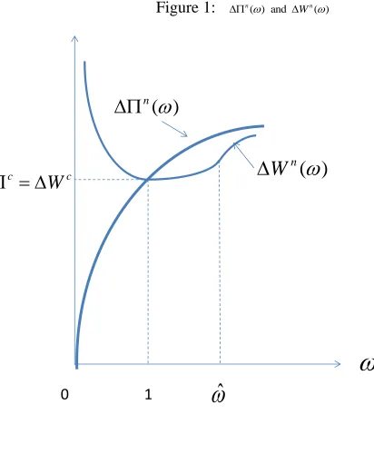
following Lemma, and illustrated in Figure 1. Lemma
(i)Wn()takes a minimum, Wn(1) Wc ( ), at 1and is convex over an interval [0, ~ ] where ~ >2; Wn() as 0; for ~,Wn() is increasing and concave.
(ii) n() is strictly increasing and concave; n(0)0; n(1) c ( ). (iii) Wn()n() 1.
Proof: The proof is in an Appendix available from the authors.
The intuition for (i) was given above in our discussion following equation (21); the intuition for (ii) was given above in our discussion following equation (15).
Given the absence of commitment, both the firm and the Period 1 government recognize that in Period 2 there could be a government that gives a weight 1 to environmental damage. We assume that, in Period 1, both the Period 1 government and the firm are uncertain about the precise type of Period 2 government that will be in power ( i.e. they are uncertain about what value ω will take), and that this uncertainty is represented by the common probability density function f( ) 0 defined over 0,, 1, with
( ) 0 0,1
f and E
1. So future governments might place a higher or lower weight on environment damage than the current government, but, on average, give exactly the same weight to damage costs as the current government. We then have:Proposition 2
Uncertainty regarding the weight placed on damage by future governments:
(i) increases the welfare gains of the Period 1 government from the firm’s R&D: ˆ
[ n( )] n(1) c
E W W W ;
(iii) E[Wn( )] E[ n( )] Proof:
(i) Follows from the fact that, as shown in Lemma (i)
( ) (1) 1
n n
W W
;
(ii) Follows from the fact that n( ) is strictly concave. (iii) Follows from (i) and (ii) and Proposition 1.
If we now take account of the fixed costs of R&D, F, then Proposition 2 raises three possible policy outcomes:
(i) if E[Wn( )] E[ n( )] F, without any intervention by the government the firm will undertake R&D which the government also regards as worthwhile; (ii) if F E[ Wn( )] E[ n( )] then the firm will not wish to undertake R&D
and the government will not wish to intervene in that decision;
(iii) if E[Wn( )] F E[ n( )] then in the absence of policy intervention the firm will not undertake the R&D but the government will wish it to undertake the R&D; the government can achieve this by offering an (absolute) R&D subsidy equal to F E[ n( )] .
Proposition 3
(i) If the Period 1 government can observe F and if [ n( )] [ n( )]
E W F E then it is optimal for the government to introduce an (absolute) R&D subsidy S F
F E[ n( )] ;(ii) If the Period 1 government cannot observe F then it can always ensure that the firm makes the right R&D decision by introducing an (absolute) R&D subsidy
[ n( )] [ n( )] 0
S E W E .
(iii) S F
S with equality if F E[ n( )]This establishes the key result of this paper: if governments are unable to commit to future environmental policies, in the sense that today’s agents (the current government and firms) cannot be sure what weight future governments might attach to environmental damage costs, then this lack of commitment can justify current governments subsiding environmental R&D.
3.2.3 Some Numerical Illustrations
Finally to relate these subsidies to potentially observable financial magnitudes we express the resulting subsidies as proportions of c - the profits the firm would make from undertaking R&D if the government could commit. Denote these subsidies (as proportions of c) by SU,ST. We show in the Appendix that these depend on the value of the demand elasticity, ε, through the formulae:
; (0) 0; (1) 0.5 2
2 )
(
U U
U S S
S
(24)
[(1 )2 2]; (0) 0; (1) 0.
) 3 )( 2 (
2 )
( 1
T T
T S S
S
(25)
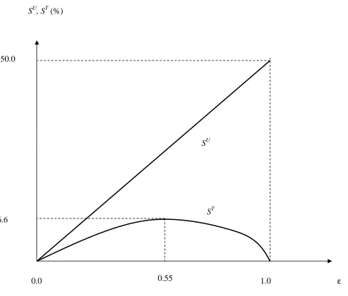
Figure 2 shows the values of these subsidies (as percentages of c) for values of ε
lying between 0 and 1. With the uniform density, the required subsidy rises from 0% to 50% of the commitment level of profit gain from R&D as the elasticity of demand, ε, rises from 0 to 1; in the mid-range of values for the elasticity of demand, 0.25 0.75 the subsidy level, SU, lies between 12% and 36%. For the triangular density, the required subsidy tends to zero as the elasticity of demand tends to 0 or 1; in the mid-range of values for the demand elasticity, 0.25 0.75the subsidy lies between 4% and 7%.
weight in the tails, and so a much great likelihood of Period 2 governments that are very different from the Period 1 government.
4. Conclusion
We have shown that the inability of governments to commit to future policies challenges the traditional prescription that environmental policies alone are sufficient to induce optimal emissions and optimal investment in R&D. This is because the inability of the current government to commit to future emission taxes increases the wish of the current government that firms undertake the investment but reduces firms’ incentives to invest.
Lack of commitment arises because governments are in power for short periods of time; have to tackle very long-lasting problems such as climate change; but cannot tie the hands of future governments. In this situation a current government faces the possibility that future governments may place a different weight on environmental damage than they do, and this for reasons entirely unrelated to the underlying economic and environmental conditions – since otherwise policies could be conditioned on these and future like-minded governments would implement them.
problems such a subsidy would be unnecessary. Our numerical results show that the required subsidies are not trivial, and depend critically on the shape of the probability distribution of future governments’ weights (on environmental damages) relative to those of the current government. The more likely it is that future governments could be very different from the current government, the higher is the required subsidy.
In demonstrating this result we have employed a very simple model. One issue is whether there may be other mechanisms by which a current government could make commitments, avoiding the need for an R&D subsidy. A number of such possibilities have been proposed in the literature: delegation of environmental policy to an independent agency, analogous to the independence of central banks in monetary policy, (Helm et al (2003)); using tradable permits linked to a financial instrument with a put option which guarantees a floor to the future price for permits (Ismer and Neuhoff (2009)). However, neither is straightforward (see Brunner et al (2012) for an excellent discussion of the relative merits of such commitment devices), particularly in the context of a long-term problem such as climate change. For example, as we have shown15, any future emission tax or permit price should be made contingent on what innovation has been carried out, so defining an appropriate floor price could be difficult; while delegation has been successful for short-term monetary policy, it would be more problematic for long-term environmental problems. Ultimately future governments could disband any such devices. A subsidy to environmental R&D by current governments is arguably a more secure way of offsetting industry’s concerns about investing in such projects.
A second issue is how robust our results would be in a richer model. There are a number of possible extensions.
One obvious extension would be to model a proper stock-externality problem with emissions also in Period 1; it is an interesting conjecture whether this could lead the Period 1 government to set too low an emission tax in Period 1 to force the Period 2 government to take more action.
A further extension would be to study a multi-country problem and consider whether joining an IEA gives a form of commitment to future emissions policy.
Thirdly we have ignored intrinsic uncertainty about the climate change process with the related issue of how the possibility of getting better information in the future about climate change damages affects current period policy in a world where governments cannot commit.
Finally we have assumed that there is just a single firm who is able to capture allReferences
Abrego, L. and C. Perroni (2002): “Investment Subsidies and Time-Consistent Environmental Policy”, Oxford Economic Papers, 54(4), 617-635.
Blackmon, G. and R. Zeckhauser (1992): “Fragile Commitments and the Commitment Process”, The Yale Journal of Regulation, 9(73), 73-105.
Boyer, M. and J-J Laffont (1999): “Towards a Theory of the Emergence of
Environmental Incentive Regulation”, Rand Journal of Economics, 30, 137-157. Brunner, S., C. Flachsland and R. Marschinski (2012): “Credible Commitment in Carbon Policy”, Climate Policy, 12(2), 255-271.
Downing, P. and L. White (1986): “Innovation in Pollution Control”, Journal of Environmental Economics and Management, 13, 18-29.
Golombek, R., M. Greaker and M. Hoel (2010): “Climate Policy without Commitment” CESifo Working Paper No 2909.
Helm, D., C. Hepburn and R. Mash (2003): “Credible Carbon Policy”, Oxford Review of Economic Policy, 19(3), 438-450.
Hoel, M. (2010): “Climate Change and Carbon Tax Expectations”, CESifo Working Paper No 2966.
Ismer, R. and K. Neuhoff (2009): “Commitments Through Financial Options: an Alternative for Delivering Climate Change Obligations”, Climate Policy, 9, 9-21. Jaffe, A., R. Newell and R. Stavins (2003): “Technological Change and the
Environment”, in K. Maler and J. Vincent (eds.) Handbook of Environmental Economics, North-Holland, Amsterdam, 461-516.
Montero, J-P, (2011) “A note on environmental policy and innovation when governments cannot commit” Energy Economics 33(1), S13-S19.
Petrakis, E. and A. Xepapadeas (2000): "Location Decisions, Environmental Policy and Government Commitment", in N. Georgantzis and I. Barreda (eds.), Spatial Economics and Ecosystems: The Interaction Between Economics and the Natural Environment, Series: Advances in Ecological Sciences WIT (Wessex Institute of Technology) Press. pp. 115-127.
Stern, N. (2007): Stern Review of the Economics of Climate Change, HM Treasury Ulph, A. and D. Ulph (1997), “Global Warming, Irreversibility and Learning”, Economic
Journal, 107, 636-650.
Ulph, A. and D. Ulph (2001) “Strategic Trade and Industrial Policy in Dynamic Oligopolies – the True Value of Commitment”, mimeo, University of Southampton.
Figure 1:
n( ) and Wn( )0
1
( )
n
( )
n
W
c c
W
ˆ
[image:28.612.42.531.85.501.2]
Figure 2: Required Subsidies with Uniform and Triangular
Density Functions as Functions of Demand Elasticity
ε SU
ST
0.0 1.0
SU, ST(%)
50.0
6.6