Centro de Astronomía(CITEVA), Universidad de Antofagasta, Avenida Angamos 601, Antofagasta, Chile 4
Department of Astronomy, Cornell University, Ithaca, NY 14850, USA 5
Instituto de Astrofísica de Andalucía(CSIC), Glorieta de la Astronomá s/n, E-18008 Granada, Spain 6
UK Astronomy Technology Centre, Royal Observatory Edinburgh, Blackford Hill, Edinburgh EH9 3HJ, UK 7
Núcleo de Astronomía, Facultad de Ingeniería y Ciencias, Universidad Diego Portales, Av. Ejercito 441, Santiago, Chile 8
Instituto de Física y Astronomía, Universidad de Valparaíso, Av. Gran Bretaña 1111, Playa Ancha, Casilla 5030, Chile Received 2019 February 4; revised 2019 May 30; accepted 2019 June 25; published 2019 August 14
Abstract
As part of the ongoing effort to characterize the low-mass(sub)stellar population in a sample of massive young clusters, we have targeted the ∼2 Myr old cluster NGC 2244. The distance to NGC 2244 from Gaia DR2 parallaxes is 1.59 kpc, with errors of 1%(statistical)and 11%(systematic). We used the Flamingos-2 near-infrared camera at the Gemini-South telescope for deep multi-band imaging of the central portion of the cluster(∼2.4 pc2). We determined membership in a statistical manner, through a comparison of the cluster’s color–magnitude diagram to that of a control field. Masses and extinctions of the candidate members are then calculated with the help of evolutionary models, leading to the first initial mass function (IMF) of the cluster extending into the substellar regime, with the 90% completeness limit around 0.02Me. The IMF is well represented by a broken power law (dN/dM∝M−α)with a break at∼0.4Me. The slope on the high-mass side(0.4–7Me)isα=2.12±0.08, close to the standard Salpeter slope. In the low-mass range(0.02–0.4Me), wefind a slopeα=1.03±0.02, which is at the high end of the typical values obtained in nearby star-forming regions (α=0.5–1.0), but still in agreement within the uncertainties. Our results reveal no clear evidence for variations in the formation efficiency of brown dwarfs (BDs)and very low-mass stars due to the presence of OB stars, or for a change in stellar densities. Our
finding rules out photoevaporation and fragmentation of infalling filaments as substantial pathways for BD formation.
Key words:open clusters and associations: individual(NGC 2244)–stars: formation–stars: luminosity function, mass function– stars: pre-main sequence
Supporting material:machine-readable tables
1. Introduction
1.1. Young Star Clusters and the IMF
Star clusters are the primary locations of star formation and the main suppliers of stellar and substellar objects in the universe(Lada & Lada2003; Portegies Zwart et al.2010). The youngest clusters are particularly important laboratories for understanding how star formation works. They give birth to objects spanning at least four orders of magnitude in mass, from the most massive stars reaching several tens of solar masses, down to substellar objects below the deuterium-burning limit at ∼0.012Me. Richly populated young clusters therefore provide an ideal testbed in which to probe a variety of yet unsolved questions related to the formation of stars, brown dwarfs (BDs), and clusters.
The distribution of stellar masses in young clusters, or the initial mass function (IMF), has been an important subject of many observational and theoretical efforts. On the high-mass side (1Me), it can be approximated by a power-law form dN/dM∝M−α, with α=2.35 (Salpeter 1955). Below
∼0.5Me, the mass distribution is significantly flatter (see, e.g., Luhman 2012 and references therein). Although the Salpeter slope is often considered universal (see, e.g., Bastian et al. 2010; Offner et al. 2014), there are some notable
examples of young clusters where the mass function appears to beflatter, withα=1.3–1.8(Stolte et al.2006; Harayama et al. 2008; Bayo et al.2011; Peña Ramírez et al.2012; Habibi et al. 2013; Andersen et al. 2017; Mužić et al. 2017). While the
flattening of the slope could be an effect of crowding for the clusters that are several kiloparsecs away(NGC 3603, Arches, Westerlund 1) (Ascenso et al.2009), this is certainly not the case for the more nearby ones(Collinder 69,σOri, RCW 38). Employing Bayesian statistics, Dib (2014) reports significant variations in IMF parameters of eight young Galactic clusters, including the slope of the IMF on the high-mass side. Recently, Dib et al. (2017) proposed a probabilistic formulation of the IMF, where the IMF is described by a tapered power law(De Marchi et al. 2010), and each parameter of this function is represented by a Gaussian probability distribution. The authors argue that the broad distribution of the IMF parameters might reflect the existence of equally broad distributions in the star-forming conditions(e.g., Svoboda et al.2016).
between low-mass stars and BDs is typically found in the range 2–5. The range of values reflects different sources of uncertainties that contribute to the derivation of the IMF slope and the star-to-BD ratio(uncertainties in distances, ages, use of different evolutionary models, reddening laws, membership issues, small sample sizes; see, e.g., Scholz et al.2013), rather than the variations between individual clusters. Although from the observations there is no convincing evidence for strong variations in the BD production efficiency in nearby star-forming regions, theoretical expectations are somewhat differ-ent. Most of the current BD formation theories in fact predict an increased production of substellar objects in dense environments or close to very massive stars. The factors that facilitate BD formation are high gas densities (Padoan & Nordlund 2002; Bonnell et al. 2008; Hennebelle & Chabr-ier 2009; Jones & Bate2018), high stellar densities that favor BD formation through ejections(Bate2012), and the presence of massive stars, where BDs can be formed through photoevaporation (Whitworth & Zinnecker 2004) or by fragmentation in their massive disks (Stamatellos et al.2011; Vorobyov 2013). Of the mentioned scenarios, a few give quantitative predictions of the impact of environment on the efficiency of BD production. In the scenario by Bonnell et al. (2008), where new objects form by gravitational fragmentation of gas infalling into a stellar cluster, BDs are preferentially formed in regions with high stellar density. An increase in object density by an order of magnitude would result in an increase in the BD fraction by a factor of about two. The predicted effect is more subtle in the hydrodynamical simulations of molecular cloud collapse by Jones & Bate (2018). An increase in gas density by a factor of 100 leads to BD frequencies larger by∼35%.
To explore potential environmental influences on BD formation, we have initiated a photometric study in a sample of young, massive clusters, characterized by high stellar densities and/or a substantial population of massive stars. In this sense, the environments we aim to cover are significantly different from those in nearby star-forming regions, with the exception of the Orion Nebula Cluster(ONC), the only site of massive star formation within 500 pc from the Sun. The latest results from the ONC show a bimodal form of an IMF, with a secondary peak in the substellar regime(Drass et al.2016). The authors interpret the substellar peak as possibly formed by BDs ejected from multiple systems or circumstellar disks at an early stage of star formation. The spectroscopic confirmation of this result, however, is still pending. In thefirst paper resulting from our study of massive clusters, we studied the core of RCW 38, a young (1 Myr), embedded cluster located at a distance of 1.7 kpc (Mužićet al. 2017). RCW 38 is characterized both by high stellar densities (core stellar surface density Σ∼2500 pc−2, i.e., twice as dense as the ONC and more than ten times denser than NGC 1333; Mužićet al.2017)and by a substantial population of massive OB stars (60 OB candidates in total, and a dozen in our small field of view of 0.5×0.5 pc2; Wolk et al.2008; Winston et al.2011). Given these characteristics, and the absence of more extreme environments that are close enough to allow the detection of BD candidates, this cluster was thought to be a good starting point in which to look for possible environmental differences in the substellar regime. Unlike what has been reported for the ONC, we found that RCW 38ʼs IMF is consistent with those in
nearby star-forming regions (α∼0.7 for the range 0.02–0.5Me).
1.2. NGC 2244
In this second paper of the series, we present the observation of the young cluster NGC 2244, located at the center of Rosette Nebula, one of the most prominent features of the Mon OB2 Cloud. The cluster contains more than 70 massive OB stars, which are presumed to be responsible for the evacuation of the central part of the nebula (Román-Zúñiga & Lada 2008). Estimates of the distance to NGC 2244 vary from 1.4 to 1.7 kpc (Ogura & Ishida1981; Perez et al.1987; Hensberge et al.2000; Park & Sung2002; Lombardi et al.2011; Martins et al.2012; Bell et al.2013; Kharchenko et al.2013), whereas most authors agree on∼2 Myr for the age of the cluster (Perez et al.1987; Hensberge et al.2000; Park & Sung2002; Bell et al. 2013).
The stellar content of NGC 2244 has been extensively studied from X-ray to mid-infrared (MIR) wavelengths. The most sensitive X-ray data to date are theChandraobservations published in Wang et al.(2008). The authors identify more than 900 X-ray sources in a∼17′×17′field, of which 77% have optical or near-infrared(NIR)counterparts and are considered young cluster members. The X-ray-selected population of Wang et al. (2008)is nearly complete down to 0.5Me. The deepest published NIR data on NGC 2244 are those taken with Flamingos at the 2.1 m telescope at the Kitt Peak National Observatory, as part of the imaging survey of the Rosette complex (complete down to J∼18.5 mag; Román-Zúñiga et al. 2008). The analysis of several clusters in the complex reveals NGC 2244 to be the largest one. That paper, however, deals with the entire Rosette complex, and does not present further specific analysis of the NGC 2244 cluster population. The early attempts to derive the IMF of the cluster reported a shallow slope α∼1.7−1.8 (Massey et al. 1995; Park & Sung2002)for stars withm>3Me, but at the same time Park & Sung (2002) cautioned about the incompleteness at the intermediate and low masses in their sample. More recently, Wang et al.(2008)derive the slopeα∼2.1 for the mass range 0.5–30Me, close to the Salpeter slope.
2. Observations and Data Reduction
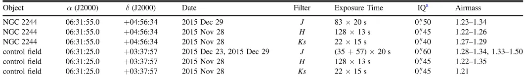
Observations of NGC2244 and another field outside the cluster area (the control field) were performed using the Flamingos-2 (F2) imager at the Gemini-South telescope (Eikenberry et al. 2004), with the program number GS-2015B-Q-46. The F2 camera provides a circularfield of view (FoV)with a radius of∼3 2 and a pixel scale of 0.18 arcsec per pixel, meaning that the instrument becomes critically sampled in very good seeing conditions. For the guiding, only the Peripheral Wavefront Sensor(PWS2)was available at the time of our observations. PWS2 vignetted part of the FoV in our observations, and these parts of the detector were masked during the data reduction. The data in J-, H-, and Ks-bands were obtained in queue mode in 2015 November and December. All the observations were taken at 70-percentile conditions for image quality, and 50-percentile cloud cover ( i.e.,J-band image quality better than 0 6 70% of the time and photometric sky at least 50% of the time).9The summary of the observations is given in Table1.
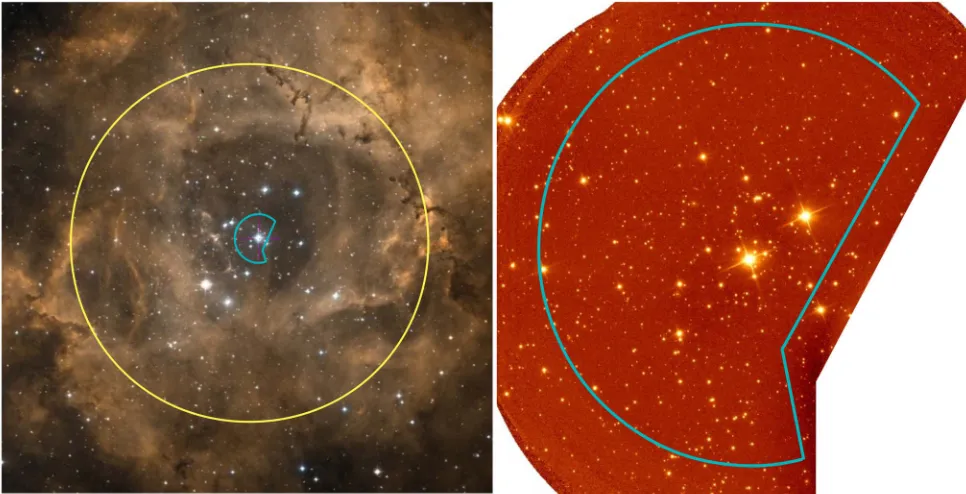
A control field was observed to estimate the degree of contamination byfield stars. A suitable controlfield should be far enough from the cluster not to contain any of its stars, yet close enough to trace the same background population. We selected a field located away from the main molecular cloud emission of the Rosette complex (see Figure2 of Román-Zúñiga et al.2008). Thefield is located ∼1°. 3 from the center of NGC 2244, along the line parallel to the Galactic plane.
Standard near-infrared data reduction techniques were applied using our home-brewed IDL routines, including dark subtraction, sky subtraction,flat-fielding, bad-pixel correction, and mosaic construction by a simple shift-and-add. Due to dithering and vignetting by the PWS2, the constructed mosaic varies in depth across thefield. To avoid issues with different photometric completeness limits, we constrain the analysis only to the part of the mosaic constructed from the maximum number of frames in all three bands, spanning the area of∼11.1 arcmin2. The Ks-band image of the observed region of NGC 2244 is shown in Figure1.
3. Data Analysis
3.1. Photometry
The photometry was performed using the DAOPHOTII/ ALLSTAR PSF-fitting algorithm (Stetson 1987), with a Gaussian PSF that varies quadratically with position in the frame(VARIABLE PSFparameter set to 2). We excluded all the
sources with the DAOPHOT sharpness parameter ∣ ∣sh >0.7, which helps to get rid of galaxies, clumps, knots, and spurious detections caused by ghosts in our images. The photometric zero-points and color terms were calculated from a comparison with the data from the United Kingdom InfraRed Telescope Infrared Deep Sky Survey (UKIDSS; Lawrence et al. 2007) Galactic Plane Survey (Lucas et al. 2008) Data Release 10. This catalog was chosen because of its photometric depth, which allows a significant overlap with the F2 source lists. The photometric uncertainties provided by the UKIDSS pipeline only include random photon noise error, and are therefore underestimated. We use a relation provided by Hodgkin et al. (2009)to calculate more realistic photometric errors that also include the systematic calibration error component. Stars with counts surpassing the linear regime of the F2 detector were excluded from the comparison. The transition to the nonlinear regime occurs atJ∼15 mag,H∼16 mag, andK∼15 mag. To avoid potential issues due different spatial resolutions of the F2 and UKIDSS data, we have discarded those sources with a neighbor at a distance <1 0 and brightness contrast ΔH<2 mag. Furthermore, we have rejected objects with uncertainties larger than 0.1 mag in the UKIDSS data or in the F2 instrumental magnitudes. Finally, the photometric zero-points and color terms were calculated using the following equations:
= + + *
-= + + *
-= + + *
-J J c J K
H H c J K
K Ks c J K
ZP ZP
ZP .
1
instr 1 1
instr 2 2
instr 3 3
( )
( )
( )
( )
For the clusterfield, the zero-points and the color terms are ZP1=25.07±0.02, ZP2=25.25±0.02, ZP3
=24.68±0.03, c1=0.06±0.02, c2 =0.04±0.02, and
c3=−0.08±0.03. For the control field we obtain ZP1=25.00±0.04, ZP2=25.28±0.04, ZP3
=24.64±0.05, c1=0.05±0.04, c2=−0.01±0.04, and c3=−0.06±0.05. The photometric uncertainties were cal-culated by combining the uncertainties of the zero-points and color terms, and the measurement uncertainties supplied by
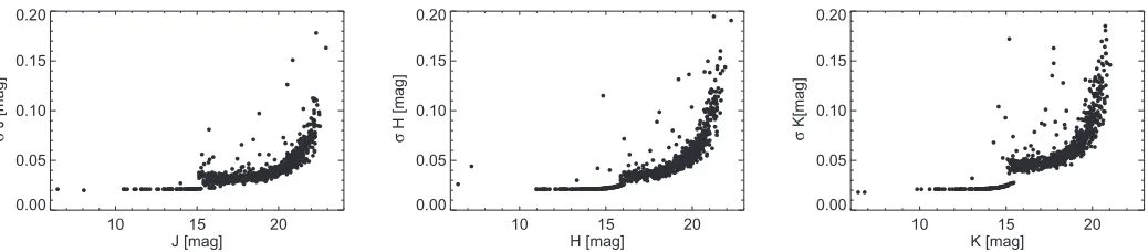
DAOPHOT, and are shown in Figure2for the clusterfield. The median uncertainties of the F2 photometry are 0.04 mag in J-and H-bands and 0.05 mag in theK-band. The photometry of the nonlinear stars was replaced by the UKIDSS measurements, with the exception of the two brightest stars in thefield which are saturated even in UKIDSS. Their photometry was taken from the Two Micron All Sky Survey(2MASS, Skrutskie et al. 2006), and transformed to the UKIDSS photometric system using the relations given in Hodgkin et al.(2009). Finally, we removed all the sources identified as galaxies in the UKIDSS catalog, verifying visually that they are not resolved into
Note.
a
Image quality(stellar FWHM measured in the reduced images).
9 http://www.gemini.edu/sciops/telescopes-and-sites/
[image:3.612.40.571.75.156.2]multiple sources in F2 images (eight galaxies removed). The
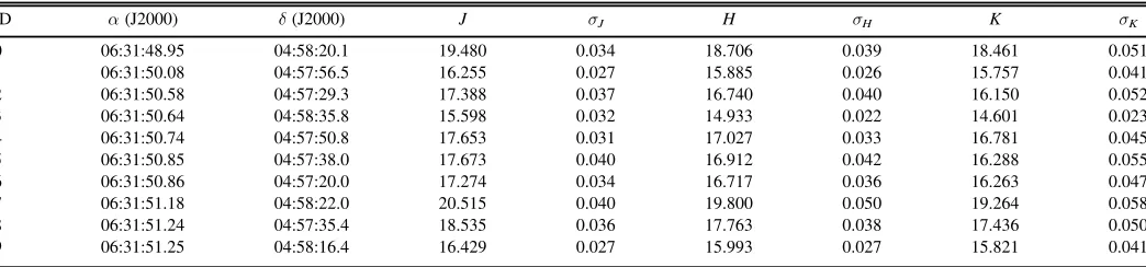
finalJHKcatalog contains 793 objects(Table2).
The completeness of the photometry was assessed with an artificial star test. Artificial stars were added to the original image using DAOPHOTʼs function ADDSTAR. The resulting image was then used as the input for a routine identical to the one used to obtain the photometry for the cluster and the control field (Section 3.1), using the same PSF solution. We inserted only 50 stars at a time to avoid crowding, and repeated the procedure 40 times at each magnitude(in steps of 0.2 mag) to improve statistics. The ratio between the number of recovered and inserted artificial stars is plotted against magnitude in Figure 3 for both the cluster (black lines) and the controlfield(blue lines). The 90% completeness limits are J=21.7 mag, H=20.9 mag, and K=20.2 mag for NGC 2244, and J=21.7 mag, H=21.1 mag, and K=20.1 mag for the controlfield.
3.2. Distance to NGC 2244 fromGaiaDR2
The distance to NGC 2244 was previously estimated to be between 1.4 and 1.7 kpc (Ogura & Ishida 1981; Perez et al. 1987; Hensberge et al. 2000; Dias et al. 2002; Park & Sung 2002; Lombardi et al. 2011; Martins et al. 2012; Bell et al. 2013; Kharchenko et al. 2013). The recently published Gaia Data Release 2 (DR2, Gaia Collaboration et al. 2018) provides precise positions, proper motions, parallaxes, and G-band magnitudes for more than 1.3 billion sources. We queried theGaiaDR2 catalog within 10′radius from the brightest star in the field(HD 46150; 06:31:55.52,+04:56:34.3). This area contains the region observed with F2, but covers a much larger portion of the cluster. The resulting list contains 3498 objects. We then cross-matched theGaiaDR2 result with the catalog of 718 clusters members from Meng et al. (2017), constructed
based on X-ray detection, infrared excess, proper motion, optical color selection, and a cut-off in the clustrocentric distance. The total number of matched sources with a valid
five-point astrometric solution is 528.
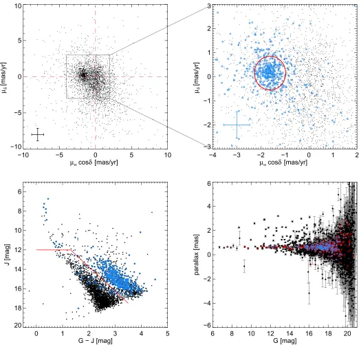
The proper motions of the Gaia sources in the field are shown in the top panels of Figure 4. There is a distinct overabundance of sources close to the positionμα,μδ≈(−1.5, 0.2)mas yr−1, corresponding to the location of the cluster members. An enlarged version of this plot is shown in the upper right panel, with the blue open circles marking the matched members from Meng et al.(2017). The mean proper
motion of the matched members is
μα=−1.62±0.65 mas yr−1 and
μδ=0.15±0.70 mas yr−1.
[image:4.612.64.547.54.301.2]The color–magnitude diagram (CMD) of the same set of sources constructed by matching theGaiaDR2 to the UKIDSS survey shows the probable member sequence clearly standing out to the right of the bulk of thefield stars. We can therefore use the proper motions and the position in the CMD as criteria to assign cluster membership. To consider a source a member in this exercise, we require it to be located inside the red ellipse in the proper motion space, to the right of or above the dividing line in the CMD, and to be classified as a star in UKIDSS (class=−1). The semimajor and semiminor axes of the red ellipse are equal to 1σwidths of the proper motion distributions in R.A. and decl. The transition from the pre-main sequence to the main sequence at the age of NGC 2244 occurs roughly at J=12(see Figures 16 and 8), motivating the horizontal red line. After applying the cuts mentioned above, we keep 345 out of the initial 3498 sources. These 345 sources are shown with red open circles in the parallax plot in the lower right panel of Figure4. 242 of the 345 selected sources belong also to the members list of Meng et al. (2017). We note that our criteria may cause us to miss some members (mainly due to the
relatively narrow allowed proper motion space, especially considering individual proper motion uncertainties), but the idea here is to minimize the number of interlopers that could bias our distance analysis, rather than to do a sophisticated membership analysis at this point.
We estimate the distance to the cluster through a maximum likelihood procedure (see, e.g., Cantat-Gaudin et al. 2018), maximizing the following quantity:
v s
ps
v s
µ v = -
-v v
P d, 1
2 exp 2 , 2 i i i i d 2 1 2 i i i 2 ⎛ ⎝ ⎜ ⎜⎜ ⎞ ⎠ ⎟ ⎟⎟
(
)
( ∣ ) ( )where P(vi∣d,svi) is the probability of measuring a valueϖi for the parallax of star i, if its true distance is d and its measurement uncertainty issvi. Here we assume that there are no correlations between individual parallax measurements, and that the likelihood of the cluster distance can be represented as the product of the individual likelihoods of all its members. We neglect any cluster spread, i.e., all the stars are assumed to be located at the same distance, which should have a negligible effect on our distance determination, given the relatively large distance to the cluster. In this way we obtain a distance to NGC 2244 of d=1.59±0.02 kpc. If we restrict ourselves only to the members identified by Meng et al.(2017)that also pass our cuts(242 objects), we obtain a very similar value of d=1.57±0.02 kpc. Our distance estimate is in agreement with the most recent value 1.55-+0.090.1 kpc from Kuhn et al. (2019), derived also from theGaiaDR2 data and assuming the systematic parallax uncertainty of 0.04 mas.
It has been shown that Gaia DR2 parallaxes suffer systematic uncertainties, with a global zero-point offset of
−0.029 mas (Arenou et al.2018; Lindegren et al. 2018; Luri et al.2018). However, applying this correction to small areas is not advisable, since the local variations can be significantly different (Arenou et al. 2018). Moreover, a low number of observed QSOs prevents a calculation of the local bias close to the Galactic plane. Arenou et al. (2018) report a median systematic offset in parallax of ∼−0.065 mas for the cluster samples of Kharchenko et al. (2013) and Dias et al. (2002), with a dependence on cluster distance and stellar colors. Judging from the right panels of Figure 16 of Arenou et al. (2018), an appropriate offset value for NGC 2244 is
∼−0.08 mas, i.e., the Gaia distance derived here might be overestimated by∼180 pc, or 11%. Considering this potential systematics, it might seem that the distance constrained by
Gaiadoes not provide a significant improvement with respect to previous measurement; however, we have to keep in mind that this is only the second data release, and that by the end of the mission, the systematics are expected to be at a microarcsecond level even at distances of a few kiloparsecs. To understand the effect this uncertainty might have on the results, we will report them for two values of the distance, 1.6 and 1.4 kpc.
As a side note, in the bottom left panel of Figure4, there is a group of relatively bright sources not recognized as members by Meng et al.(2017), located to the right of and above the red lines (roughly J<13 and G−J>1). Only about 10% of these sources pass all our membership cuts. The parallaxes of those that do not, signal that they are mostly located behind the cluster, and their position in absolute CMDs is consistent with a giant branch. About a quarter of these objects have been observed by the LAMOST survey,10and have determinations of surface gravity (logg) and effective temperature (Teff).
About 75% of those haveTeff=4500–5000 K and logg<3, i.e., they are background giants.
4. Identification of Cluster Members and the IMF
4.1. Outline
Since this is a long and relatively complicated section, here we present a short summary of the methodology, giving readers a chance to skip some sections that might be too technical or detailed.
1. The goal of this sectionis to derive the IMF and the star-to-BD number ratio for NGC 2244(Sections4.4and4.5). The results are presented for three different isochrones and two distances (1400 and 1600 pc), in order to estimate the effect that different assumptions have on the results.
[image:5.612.49.568.49.163.2]2. Membership determination(Section4.2). Thefirst step in the analysis is to separate cluster stars from the contaminants sharing the same line of sight. For the sources brighter thanJ∼18, this can be done using the color, proper motion, and parallax cuts on theGaiaDR2 andPan-STARRSdata(Section4.2.1). However, our NIR catalog extends more than 3 mag deeper, and in this regime we employ a statistical determination of member-ship, comparing the CMD of the population observed in direction of the cluster to that of the control field (Section 4.2.2). In this procedure, there are several parameters that are varied (cell sizes and positions,
Figure 2.Photometric uncertainties as a function of magnitude inJ(left),H(middle), andK(right), for the cluster data set. Photometry of the bright sources whose photon counts exceeded the linearity limit of the detector was replaced with the photometry from UKIDSS or 2MASS, causing the discontinuity.
10
difference in extinction between the cluster and the control field), and each combination of these parameters can give a slightly different solution. We keep all the possible solutions(324 member lists)and use them later to evaluate the uncertainties that this approach introduces to the IMF and star-to-BD ratio.
3.Isochrones(AppendixA). Stellar parameters are derived in comparison to theoretical models. The basic products of the stellar models are the bolometric luminosity and effective temperature, which are converted into magni-tudes and colors, by applying bolometric corrections and Teff–color relations. The conversion can be done by using
the atmosphere models or empirical relations. Here we decide to test both approaches, and we derive our results using three different isochrones.
4.Derivation of stellar parameters (Section 4.3). We compare three different methods to derive effective temperature, mass, and extinctions. The first method is based on fitting the spectral energy distribution (SED) over a large wavelength range (optical to mid-infrared, where available; Section 4.3.1). The other two methods explore the derivation of parameters from the three NIR colors only (JHK), in one case assuming that the observed colors are photospheric (Section 4.3.2), and in the other case assuming that some intrinsic excess at the NIR wavelengths is present(Section4.3.3). Wefind that
the results are consistent with each other, validating the use of only NIR magnitudes and colors in mass determination at the faint end, where this is our only option(Section4.3.4).
4.2. Cluster Membership
4.2.1.GaiaDR2 and Pan-STARRS1
For the brighter portion of sources in ourfield of view, data from Gaia DR2 and Pan-STARRS1 (PS1; Chambers et al. 2016)are available. 199 sources from ourJHKcatalog have a counterpart with afive-parameter astrometric solution in Gaia DR2 (down to J≈17.5−18) within the matching radius of 0 5. The average distance between the matched entries in the two catalogs is 0 03, justifying our choice of the relatively small matching radius. We consider a source to be member candidate if it satisfies the following criteria, as depicted in Figure5:(1)it is located above and to the right of the red lines in theJ,(G−J)diagram(open gray circles in top panels);(2) its 1σ proper motion errors intersect the circular area with a radius of 1.5 mas yr−1, centered at the average value of the proper motions derived in Section3.2(red circle in the top right panel);(3)its 1σerrors in parallax intersect one of the red lines plotted in the bottom left panel (marking 1.4 and 1.7 kpc distance, see Section 3.2). In total 72 of 199 sources pass our cuts and are considered member candidates. They are marked with orange diamonds in the bottom right panel of Figure5.
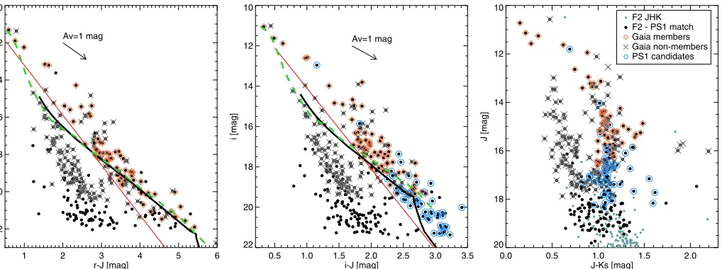
[image:6.612.46.568.74.196.2]PS1 contains neither proper motions nor parallaxes, but its optical photometry is deeper thanGaia, and can further help in selection of candidate members. As shown in the left and middle panels of Figure 6, the sources are separated in two bands when combining optical with NIR photometry.11Orange diamonds mark the member candidates selected byGaia, and gray crosses those rejected in the same procedure. Following the sequence of theGaiamember candidates, we draw dividing lines in r,(r−J)and i,(i−J) CMDs(solid red lines). We select the sources not classified byGaiaand located to the right of the red lines in both diagrams as member candidates(blue open circles). 47 out of 362 F2–PS1 matches(matching radius 0 5) with valid r or i magnitudes are selected in this way. Judging from theGaiacolor versus astrometric selection,∼15
Table 2
Near-infrared Photometry of Sources in the NGC 2244 Field Covered by Flamingos-2 Observations
ID α(J2000) δ(J2000) J σJ H σH K σK
0 06:31:48.95 04:58:20.1 19.480 0.034 18.706 0.039 18.461 0.051
1 06:31:50.08 04:57:56.5 16.255 0.027 15.885 0.026 15.757 0.041
2 06:31:50.58 04:57:29.3 17.388 0.037 16.740 0.040 16.150 0.052
3 06:31:50.64 04:58:35.8 15.598 0.032 14.933 0.022 14.601 0.023
4 06:31:50.74 04:57:50.8 17.653 0.031 17.027 0.033 16.781 0.045
5 06:31:50.85 04:57:38.0 17.673 0.040 16.912 0.042 16.288 0.055
6 06:31:50.86 04:57:20.0 17.274 0.034 16.717 0.036 16.263 0.047
7 06:31:51.18 04:58:22.0 20.515 0.040 19.800 0.050 19.264 0.058
8 06:31:51.24 04:57:35.4 18.535 0.036 17.763 0.038 17.436 0.050
9 06:31:51.25 04:58:16.4 16.429 0.027 15.993 0.027 15.821 0.041
[image:6.612.45.292.236.394.2](This table is available in its entirety in machine-readable form.)
Figure 3.Completeness of the F2 photometry calculated with an artificial star
experiment for NGC 2244(black)and the controlfield(blue). Different line styles represent different photometric bands: full, dashed, and dotted lines for J-,H-, andK-bands, respectively.
11
of these sources might still be interlopers. The selected sources are identified in Table3.
The selection usingGaiaand PS1 is nearly complete down toJ∼18.5. About 6% of the F2 sources with J<18.5 (21/ 337)cannot be classified as members or non-members in this way, because no counterpart with valid r or i magnitude is found in PS1, or no astrometry is given inGaia. Most of these sources are located very close to the two brightest stars in our FoV, which might have affected their measurements in Gaia or PS1.
[image:7.612.45.567.48.549.2]We matched the sources selected in this section with the member list of Meng et al. (2017), who select as member candidates all sources detected in both X-rays and Spitzer/ IRAC, or those that show excess at wavelengths of 8–24μm. The depth of their survey seems to be fairly complete down to the 2MASS completeness limit at J=15.8 mag, and we restrict the comparison down to that value. Of the 61Gaia/PS1 selected candidates brighter thanJ=15.8, 47 are found in the member list of Meng et al. Of the 14 sources that are not in their list, 10 are not in the X-ray/NIR combined catalog of Wang et al.(2008), which was used for selection in the former
work. The remaining four objects were observed by Spitzer (Balog et al. 2007), but they do not show an excess at these wavelengths, which is possibly the reason why they were rejected by Meng et al. (2017). On the other hand, of the 59 objects rejected byGaia/PS1, 20 are found in the member list of Meng et al. Of these 20, six were rejected based on either colors or proper motions, and the remainder based on parallax. It might be worth noting that the relative error of the parallax for these sources is relatively large(median∼0.3), but only for
four of them do the lower and upper bounds of the distance confidence interval fromGaiaDR2(Bailer-Jones et al. 2018) agree with the distance to NGC 2244.
4.2.2. Flamingos-2
[image:8.612.46.565.46.562.2]Our F2JHKphotometry extends more than three magnitudes inJdeeper from the objects detected in PS1. In the magnitude range covered by Gaia/PS1 the probable member sequence separates nicely from the background even in the NIR CMD,
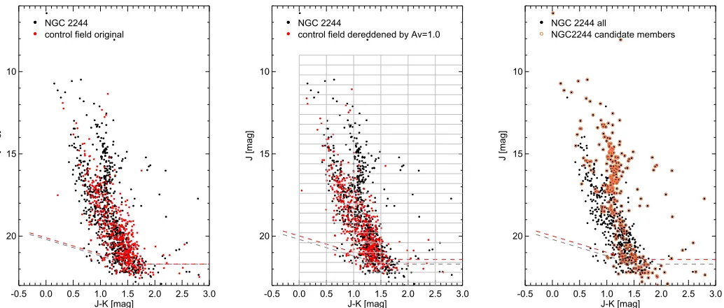
but belowJ∼17 the cluster members occupy the same space in the CMD as the foreground and backgroundfield stars. To estimate the relative contribution of the contaminants to the stellar sample observed in the direction of the cluster, we compare the cluster CMD with that of the control field (see Figure7). The method is similar to the one we applied to the cluster RCW38 (Mužić et al. 2017) but includes a few modifications. The main steps of the method are as follows.
1. The CMD is subdivided into grid cells with a step size (Δcol, Δmag) in the color and magnitude axes, respectively.
2. For each CMD cell, we calculate the expected number densities of stars in the clusterfield and the controlfield. The number density of field stars has in principle to be scaled to account for different on-sky areas covered by the images, although in our case this number is close to one.
3. A number of objects corresponding to the expectedfield object population is then randomly removed from corresponding cells of the cluster CMD.
To calculate the number densities of stars in each cell, we use the method outlined in Bonatto & Bica(2007). Each star is represented by a Gaussian probability distribution of magnitude and color, with the widths determined by the uncertainties. The expected number density of stars in each cell is calculated as the sum of each individual star’s probability of being in a corresponding cell. In this way we take into account the fact that stars with large uncertainties have a non-negligible probability of populating more than one CMD cell.
The choice of the cell size is an important parameter to take into account, and results from a compromise between having a sufficient number of stars in each cell and preserving the morphology of different CMD evolutionary sequences. We have tested the cell size of Δcol=(0.4, 0.5, 0.6) mag and Δmag=(0.4, 0.6, 0.8) mag. Furthermore, for each combina-tion of the color and magnitude cell sizes, we repeat the procedure with the grid shifted by±1/3 of the cell width in each dimension. This results in 81 different configurations.
The control field population seems to have, on average, a slightly higher extinction than the cluster field. This can be appreciated by looking at the upper sequence in the CMD, where there is a slight shift between the sequence of the cluster on the left and the controlfield. We estimate that the difference is somewhere in the range 0.5–1 mag. The control field sequence is therefore dereddened at the beginning of the procedure by ΔAV=(0.5, 1.0)mag. Finally, we applied the procedure to both theJ,(J−H)andJ,(J−K)CMDs. In total, this procedure results in 81×2×2=324 different member lists, which can then be used to calculate statistical errors of the IMF and the star-to-BD number ratio, which are introduced by the decontamination procedure.
We estimate that(61±2)% of the sources observed toward the cluster are actually field contaminants. The number of cluster stars surviving the procedure is 310±18 (the uncertainty is the standard deviation of the 324 outcomes of the above procedure).
Our procedure successfully recovers the member sequence at J17 mag, which appears separated from the field objects located to the left(see Figure8). Green diamonds in this plot show the candidate members from theGaiaand PS1 selection.
4.3. Derivation of Stellar Parameters
[image:9.612.60.569.50.240.2]In this section we explore different approaches to derive stellar effective temperatures, masses, and extinction (AV) of candidate members of NGC 2244 from multi-band photometry. For the candidate members selected with the help ofGaiaand Pan-STARRS1, we can take advantage of the existence of photometry over a large wavelength range, and derive these parameters by fitting their SEDs to the synthetic photometry obtained from atmosphere models. This, however, only works for the bright part of our catalog. For the objects withJ18.5 where we only have JHK photometry available, the two-parameter SED fitting becomes degenerate. Instead, to simultaneously derive the extinction and the masses of the cluster members, we compare the JHK photometry to model isochrones. The first approach here is to assume that the observed colors come from the reddened stellar photosphere.
However, as argued by Cieza et al. (2005), classical T-Tauri stars(CTTSs)can present an excess already in theJ-band, and therefore a simple dereddening of the photometry to the model isochrones can overestimate the extinction, and consequently also the stellar luminosity and mass. About 70% of the stellar members of NGC 2244 host dusty disks or envelopes (Meng et al. 2017), which can contribute some excess flux to their near-infrared colors. For this reason we also develop a method that takes into account this possible intrinsic excess when deriving the extinction toward individual stars in the cluster.
Throughout this section, we assume an age of 2 Myr(when employing the isochrones; Perez et al. 1987; Hensberge et al. 2000; Park & Sung 2002; Bell et al. 2013), and adopt the extinction law from Cardelli et al. (1989) with the standard value of the total-to-selective extinction ratio RV=3.1 (Fernandes et al. 2012). For a detailed description of the isochrones used in Sections 4.3.2and 4.3.3, see Appendix A. We derive the parameters assuming the cluster distance of 1.6 kpc derived from the Gaia data, and use this for the comparison of the different methods. At the end, we also derive the masses for the distance of 1.4 kpc, which should be a lower limit on the distance judged from the Gaiasystematics.
4.3.1. Optical to Near-infrared SED Fitting
We construct the SEDs of theGaia/PS1 candidate members using the available optical and NIR photometry mentioned in the previous sections. We also use the Spitzer/IRAC photo-metry from Balog et al.(2007)where available, but only for the sources not showing excess at mid-infrared wavelengths (15 sources). Whether a source exhibits an excess was determined with the help of the tool VOSA (Bayo et al. 2008), which detects mid-infrared excess based on the slope of the infrared SED. The validity of this selection was also visually inspected. We retrieved the BT-Settl atmosphere models (Baraffe et al. 2015)for loggvalues of between 3.5 and 4.5, andTeffbetween
2000 and 25,000 K12 and interpolate the models to the intermediate loggvalues of 3.75 and 4.25(young stars with an age of up to a few million years and masses below 10Me should have loggbetween 3.5 and 4.25). The metallicity is set to the solar value. The extinction was varied between 0 and 10 in steps of 0.1 mag. Wefind the model best matching the data by minimizing the χ2parameter calculated as
å
cs
= - ´
=
F_ D F_
_ , 3
i N i i i 2 1
obs model 2
obs 2
( )
( )
where Fobs and Fmodel are observed and model fluxes,
respectively, and σobs are observed flux uncertainties. D is
the dilution factor,D=(R/d)2, withRbeing the stellar radius anddthe cluster distance(fixed to 1600 pc). The value ofRis
fixed for each combination ofTeffand loggand was extracted
from the models. This is motivated by the relation
= ´
R G m g, wheremstands for the object’s mass, which is directly related to Teff at a particular value of logg. We
visually inspected all thefits, and rejected two of them due to a clear discrepancy between the observed and the best-fit model
fluxes. In Figure 9 we show a subset of the object SEDs, together with the best-fit model synthetic photometry(red). In the leftmost panels we show two objects with optical to near-infrared photometry, in the middle panels those with no excess in Spitzer photometry, and in the rightmost panels those showing the excess(the excess points were not used tofit the SED). The best-fit parameters are given in Table3.
Finally, the masses were obtained by interpolating the Teff–mass relation from the 2 Myr models to the best-fit Teff
values.
4.3.2. From NIR Colors, without Excess
In this section we derive the stellar parameters by using only the JHK photometry, assuming that the colors are coming directly from the stellar photosphere, i.e., the objects present no excess due to dusty disks in the NIR. To simultaneously derive Teff, masses, and AV of the cluster members, we simply deredden the photometry in the J, (J−H) diagram to the isochrones(see Figure8). We also check the source position in the color–color diagram(CCD; right panel in Figure8), where the solid blue line represents evolutionary models and the dotted red lines are the reddening vectors. If a source is not located in a strip defined by the two reddening lines encompassing the region compatible with evolutionary models (two dotted red lines to the left, region A), then the parameters cannot be derived.
[image:10.612.44.567.75.146.2]To estimate the effect that the photometric uncertainties have on this determination of extinction and mass, we apply the Monte Carlo method: for each source we create a set of 1000 magnitudes in each band, assuming a normal distribution with a standard deviation equal to the respective photometric uncertainty. For each of the 1000 realizations we then derive the mass, Teff, and AVby dereddening the photometry to the isochrone. The final AV for each source is calculated as an average, and its uncertainty as the standard deviation of all realizations. The resulting mass distributions, however, in most cases will not be well represented by a normal distribution because the magnitude is not a linear function of mass. The
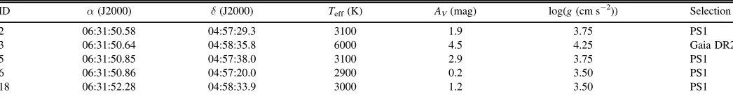
Table 3
Member Candidates fromGaiaDR2 and PS1, along with the Best-fit Parameters from the SED
ID α(J2000) δ(J2000) Teff(K) AV(mag) log(g(cm s−2)) Selection
2 06:31:50.58 04:57:29.3 3100 1.9 3.75 PS1
3 06:31:50.64 04:58:35.8 6000 4.5 4.25 Gaia DR2
5 06:31:50.85 04:57:38.0 3100 2.9 3.75 PS1
6 06:31:50.86 04:57:20.0 2900 0.2 3.50 PS1
18 06:31:52.28 04:58:33.9 3000 1.2 3.50 PS1
(This table is available in its entirety in machine-readable form.)
12
resulting mass distributions are typically skewed toward higher masses, meaning that by taking a mean of all the realizations as the final mass, we might in fact be overestimating it. For this reason, we save the resulting mass and Teff distributions for
each source. These distributions are later used to estimate the confidence interval for mass andTeffwhen comparing different
derivation approaches, and to draw masses in the Monte Carlo simulation used to determine the IMF.
4.3.3. From NIR Colors, with Excess
In this section we derive the stellar parameters by using only the JHK photometry, but this time allowing that some of the objects might have an intrinsic NIR excess. While this method makes various assumptions concerning the disk properties, it also might be more realistic, given the large disk fraction in the cluster. Figure 8shows the CMD and the CCD used to derive the source extinction and masses. To estimate the effect that the photometric uncertainties have on our determination of extinction and mass, we apply the same Monte Carlo method as in the previous section, only using a different method to derive individualTeff, mass, andAV, consisting of the following steps.
1. We first check the source’s position in the CCD. In Figure 8(c), the solid blue line represents evolutionary models, the solid and dashed orange lines the locus of T-Tauri stars and the corresponding uncertainties(Meyer et al. 1997). The dotted red lines are the reddening vectors, encompassing the regions where the colors are consistent with reddened evolutionary models or CTTSs (region A), and CTTSs only(region B).
2. Each star is represented by a distribution of colors determined by the value of photometry and the corresp-onding uncertainty (sampled 1000 times), which will typically fall into different regions of the CCD. If a point falls into region A, but below the CTTS locus, the
extinction and corresponding mass are derived by dereddening the photometry to the isochrone in the J, (J−H) CMD (case1). In region B, the extinction is derived by dereddening the colors to the CTTS locus (case2; Meyer et al.1997). If the object falls to the left of region A or to the right of region B, the extinction and mass cannot be derived.
3. Incase2, in addition to the interstellar extinction, we also correct for an excess due to the circumstellar disk or envelope, chosen randomly in the interval rJ=0–0.7 mag for the J-band and rH=0–1.1 mag for theH-band(Cieza et al.2005),13with a conditionrH>rJ (Meyer et al. 1997). If a point falls into region A but above the CTTS line (named A1 in the following), we have two options: deredden the photometry to the isochrone (as in case1) or to the CTTS locus (as in case2). To decide, we first look at in what fraction of 1000 realizations a star’s photometry ends up above the CTTS line. If this fraction is less than 70%, we apply the case2 procedure to all the points that fall into region A1. Otherwise, we randomly pick a number of points (from A1)to which thecase2 procedure would be applied, so that the total number of times we allow for an infrared excess amounts to 70%. In the remainder of the cases we apply the same procedure as in case1. The mentioned percentage is chosen to match the disk frequency of the cluster (Meng et al.2017).
4. The derived extinction is then used to convert theJ-band photometry to the absolute J-band magnitude, which directly corresponds to a certainTeffand mass as given by
[image:11.612.51.568.49.269.2]the models.
Figure 7.A demonstration of the procedure for statistical determination of membership. Here we show only one of a total of 324 realizations, which were obtained by varying several parameters, e.g., the difference in extinction between the cluster and the controlfield, cell size, etc.(see Section4.2.2for details). Left panel: CMD toward the cluster(black)and the controlfield(red). Gray and red dashed lines represent the 90% completeness limits for the cluster and the controlfield, respectively. Middle panel: here the control field has been dereddened by AV=1 to approximately match the probablefield sequence atJ−K<0.8 andJ<17. The
completeness limit for the controlfield has been modified accordingly. The grid cell size is 0.5×0.6 mag2. Right panel: we overplot(orange circles)the candidate members that“survived”the statistical CMD cleaning in this particular step.
13
4.3.4. Comparison of the Three Methods
In Figure 10, we compare the three mass/Teff methods
described in Sections 4.3.1(SEDfitting;method1 for the rest of the section),4.3.2(JHKwithout excess;method2), and4.3.3 (JHK with excess; method3). The top panels compare the results of method3 with those of method1, and the bottom panelsmethod3 withmethod2. In the left and middle panels, we show the comparison ofTeffand masses, where in the case
ofmethods2 and 3 we show only the results usingisochrone1. The Teff error bars for the SED fitting are set to 100 K,
reflecting the spacing of thefitting grid. For the methods based on JHK photometry only (methods2 and 3), we have a distribution ofTeffand masses for each object, which does not
necessarily follow the normal distribution, and in most cases is not symmetric. The Teffand mass for the plot were calculated
as the weighted average, with the weights provided by the distribution function. The error bars represent 95% confidence limits. We note that the large Teff error bars for the massive
stars in methods2 and 3 arise from the Teff/AVdegeneracy at the main-sequence transition region of the isochrones. Basically, there is more than one combination of Teff and AV that can be used to deredden a star’s photometry onto the isochrone, and the span of Teff values in this region is large
(∼14,000 K).
The right panels of Figure10show the IMFs derived using the masses obtained by different methods. The IMFs are derived in the same way as explained in the following section. For the upper plot the input object list contains the Gaia/PS1 candidate members, while in the lower plot the IMF is averaged over 324 lists resulting from the control-field-based member-ship analysis (Section4.2.2).
1. Method3 versusmethod1(top panels of Figure10): The values ofTeffobtained by the two methods are
in reasonable agreement below∼6000 K, where most of the objects are located. Above this temperature there is a
set of objects with significantly higherTefffrom theJHK
method(albeit with very large error bars). These are the objects that occupy the space in the CMD around the pre-main-sequence transition(masses roughly in the 2–6Me range, see Figure 8). Their Teff and mass distribution
tends to be bimodal, resulting in the larger error bars, and values typically higher than those obtained by the SED
fitting. There are also a handful of sources just above the smaller blue box in the left panel of Figure 10. SED
fitting for these sources prefers higherTeffandAVthan the JHK method. There is no obvious explanation for this discrepancy, but we note that most of them (4/5) are either at the faint end in Gaia and have very large parallax errors, or were selected in PS1(color selection only). They might simply be contaminants.
For the objects located inside the blue box of the top left plot of Figure 10, we obtain the average Teff
difference (method3 – method1) and its standard deviation ΔTeff =−80±310 K. The resulting IMFs
are very similar. The difference in the bin at around 3Me comes from thefive objects discussed above, where SED
fitting yields higher masses. Removing those objects, the red point becomes consistent with the black one.
To conclude, the overall good agreement between the parameters obtained by the two methods, and in particular by the similar IMFs, is reassuring, and validates the methods based onJHKcolors only. This is important, because it represents the only option to derive Teff and
mass for the fainter sources.
2. Method3 versusmethod2(bottom panels of Figure10): As expected, the method ignoring the NIR excess predicts systematically higher Teff and masses than the
method allowing for the infrared excess. The averageTeff
difference (method3 – method2) and its standard deviationΔTeff=−80±150 K. The results agree well
[image:12.612.48.567.50.267.2]within the errors, and the impact on the resulting IMF is
Figure 8.(a)J,(J−K)and(b)J,(J−H)color–magnitude diagrams, and(c)color–color diagram of all the sources detected toward NGC 2244(black dots), with the green diamonds marking the candidate members from theGaiaand PS1 selection. The blue solid line shows the 2 Myr isochrone(isochrone2)shifted to the distance of 1600 pc, while the red solid line represents the same isochrone reddened to the average extinction of the known cluster members(AV=1.5 mag). The dashed
magenta isochrone is the unreddened isochrone at the distance of 1400 pc. The solid and dashed orange lines represent the locus of T-Tauri stars and the corresponding uncertainties(Meyer et al.1997). The dotted red lines show the reddening vectors(Cardelli et al.1989), and the red crosses along the reddening lines markAV=0, 5,
minimal, and only at the lowest-mass bins. Clearly, ignoring the NIR excesses in the determination of mass does not seems to be a crucial point for studying the IMF, but anyway for the remainder of the paper we decide to use the masses derived frommethod3.
In Figure 11 we show histograms of the extinction values derived by the three methods. The top panel is comparing the AV values frommethods 2 and 3 for the objects from the full JHKsample. Note that theAVderivation relies on dereddening the photometry to the 2 Myr isochrone shifted to the distance of the cluster. The middle and bottom panels show the histograms of the three methods, but only for the objects in theGaia/PS1 sample of candidate members. The average extinction of the cluster is 1.7±1.1 mag from the SED fitting (method 1), 1.3±1.1 mag from JHK photometry without excess(method 2), and 1.4±0.9 mag from JHK photometry with excess (method3). The listed uncertainties are standard deviations of the three distributions. The extinctions derived by the three methods are in general consistent with each other, and we see no large intracluster spatially variable spread of extinctions.
4.4. Initial Mass Function
In this section we derive the IMF of NGC 2244, for masses in the range from 0.02 to 7Me. Stellar masses are binned with logarithmic bin sizes of Δlog(m/Me)=0.2. As can be appreciated from Figure8 our lower mass limit is well above the 90% completeness limit at the average cluster extinction (AV=1.5 mag), and should also contain the complete dereddened control field population to ensure the lowest-mass bins are not artificially overpopulated.
In Section 4.2 we have derived 324 lists containing statistically cleaned probable members. Each object was assigned a mass distribution using the method described in Section 4.3.3. For each of the 324 member lists, we run a Monte Carlo simulation to derive the values and uncertainties ofdN/dMfor each bin. ThedN/dMvalues of the resulting 324 IMF versions are combined (as a weighted average)to derive the final cluster IMF. The Monte Carlo simulation is very similar to the one previously applied in the cluster RCW 38
(Mužićet al.2017). The mass of each star is drawn from the distribution derived in Section 4.3.3. This is performed 100 times, and for each of the 100 realizations we do 100 bootstraps, i.e., random samplings with replacement. In other words, starting from a sample with N members, in each bootstrap we draw a new sample ofNmembers, allowing some members of the initial sample to be drawn multiple times. This results in 104mass distributions, which are used to derivedN/ dMand the corresponding uncertainties.
In the upper panels of Figures12and13we show the IMF in the power-law form (dN/dM∝M−α), derived from three different sets of isochrones and for distances of 1600 pc and 1400 pc, respectively. In all cases the IMF is well represented by two power laws, with a break at∼0.4Me. We fit separate power laws to the mass ranges 0.4–7Meand 0.02–0.4Me, as well as to the one encompassing only the substellar regime (∼0.02–0.1Me). The least-squaresfits are shown as gray lines in Figures 12and 13, and the resulting slopesα are given in Table4. For each distance, theαvalues derived from the three isochrones agree within the uncertainties. The largest variation is seen in the 0.02–0.1Merange, where thefit is more sensitive to single-point variations given the small number of points available for it. We can also observe that the uncertainty in distance of the cluster does not significantly affect our results, which again agree within the uncertainties. For a comparison, we overplot the Kroupa segmented power-law IMF, normal-ized to the total number of objects in the cluster(orange line). To estimate the effects of the choice of the bin size and location, we repeat the IMF calculation and power-law fits (within the same mass limits) for two additional bin sizes, Δlog(m/Me)=0.15 and 0.25. We also repeat the calculation with the same bin size as before(Δlog(m/Me)=0.2)but shift the bin locations by half the bin size. For each run, we combine the obtained slopes from the three isochrones as a weighted average, and we show the results in Table 5 of Appendix B. The first line in the table is the default one and is shown to facilitate the comparison. There is no major effect on the slope of the IMF in any of the considered mass ranges.
[image:13.612.115.497.51.258.2]In the lower panels of Figures12and13we plot the IMF in the log-normal form(dN/dlogM), and overplot the Kroupa and
Chabrier (Chabrier2005) mass functions, both normalized to match the total number of objects in the cluster. Unlike the power-law tail at masses >1Me, the log-normal part of the Chabrier mass function does not seem to represent the NGC 2244 mass function very well. Possible implications of this result will be discussed in Section 5.
For the masses above 0.4Me,α=2.12±0.08 is close to the Salpeter slope (α=2.35; Salpeter1955), and identical to the one derived for X-ray-selected members with masses >0.5Me (Wang et al. 2008). Below 0.4Me, a single power law with α=1.03±0.02 describes well both the low-mass stellar and substellar regimes. We can compare this with the values of other clusters and star-forming regions summarized in Table4 of Mužićet al.(2017). The slope of the low-mass IMF in NGC 2244 is steeper than the one in RCW 38(located at 1.7 kpc), where we find α=0.7±0.1 for the mass range 0.02–0.5Me. The slopes found in nearby star-forming regions at distances of up to 400 pc, typically lie in the range 0.5–1.0. The slope we derive for NGC 2244 at masses 0.02–0.4Meis at the high end of this range, but still in agreement with it, taking into account the statistical uncertainties. Furthermore, there are a number of other sources of uncertainty that are more difficult to take into account, such as the errors in age, systematics associated with the evolutionary models, extinction laws, and
finally the choice of the mass range included in the fit. The latter is demonstrated by the power-law fits in the substellar regime, which are somewhat shallower than those encompass-ing also very low-mass stars.
4.5. Star/BD Ratio
To estimate the ratio between stars and BDs, we use the masses derived in Section4.3.3and apply the same method as we did in deriving the IMF, generating 104mass distributions for each of the 324 member lists. The stellar–substellar mass boundary is set to 0.075Me, the value at the solar metallicity. We calculate the ratio using two low-mass limits on the BD side, 0.02 and 0.03Me. On the stellar side, we set an upper limit at 1Me as commonly found in the literature, but also calculate the ratio by taking into account all stellar candidates. The results are given in Table 4 for the three different isochrones used in this work. The first column contains the results for the mass ranges 0.03–0.075Me for the BDs and 0.075–1Mefor the stars, which are the limits most commonly used in the literature and the most suitable for comparison to other works. The star-to-BD number ratio in this mass range for the core of NGC 2244 is 3±0.3. Wefind that the star-to-BD ratio in NGC 2244 is slightly larger than that in RCW 38 (2.0±0.6; Mužićet al.2017); however, the values are still in agreement within their uncertainties. Furthermore, the star-to-BD ratio in NGC 1333 was found to be 1.9–2.4, and that in IC 348 was 2.9–4(Scholz et al.2013). For Cha-I and Lupus3, Mužić et al. (2015) derive the ratio of 2.5–6.0, although the analysis based on the completeness levels of the spectroscopic follow-up suggests that these ratios might in reality be on the lower side of the quoted span. These numbers are also in agreement with the star-to-BD ratios found in the ONC(3.3-+0.7
0.8 ; Andersen et al.2008)and NGC 2024(3.8-+1.5
2.1; Andersen et al.
[image:14.612.48.567.49.358.2]2008).
Figure 10.Comparison of effective temperatures(left), masses(middle), and the resulting IMF(right)derived by the three methods(see Section4.3for details). The
In Appendix C, we derive stellar surface densities for a number of young clusters and star-forming regions, and in Figure15we show the dependence of star-to-BD ratio on this parameter. Different regions are represented by polygons of different colors. The height of each polygon represents either the ±1σrange around the mean value or the range in star-to-BD ratio if given in this form. The width of the polygons has no physical meaning. The filled polygons represent the regions with few or no massive stars, while the dashed ones mark the regions with substantial OB star population. The star-to-BD ratio does not seem to depend on either the stellar density or the presence of OB stars.
To compare our results with expectations from the standard forms of mass function, we perform a simulation in which we draw 310 stars in the mass range 0.02–10Me(our estimate of the average number of members and mass limits in the data) from the underlying Kroupa or Chabrier mass functions. We then estimate the star-to-BD ratio counting the sources in the mass ranges 0.03–0.075Me and 0.075–1Me. Repeating this process 104 times, we obtain distributions of star-to-BD
to-BD ratio than the Chabrier one, which predicts higher values of the ratio than what wefind in NGC 2244.
The low-mass end IMF slope in RCW 38 is shallower than that of NGC 2244, while the star-to-BD ratio we derived for RCW 38 is lower than the one derived for NGC 2244. This is the opposite of what is expected, since a shallower IMF slope should in principle result in fewer BDs with respect to stars ( i.e., higher star-to-BD number ratio). The reason for this is the way we treated the incomplete mass bins in the survey of RCW 38. The data in the lowest-mass bins were corrected for incompleteness in the IMF calculation, according to the average K-band magnitude of the sources belonging to each bin. However, when calculating the star-to-BD ratio, all BDs are counted in a single bin and therefore this approach could not be applied. In this case we added a “missing”object for each source if its K magnitude was in the incomplete magnitude range. The mass function we derived for RCW 38 is consistent with a slightly higher star-to-BD ratio(∼4). The value is still within the range expected from other star-forming regions, but we note that the way the incompleteness is treated is clearly another important source of uncertainty. In this work, however, we do not encounter this issue since the analysis was restricted to the levels where our photometry is more than 90% complete.
5. Discussion
The main goal of this work is to study the low-mass part of the IMF and compare it with the well studied mass distributions in nearby star-forming regions and with the results of our recent study in another massive young cluster, RCW 38. According to different BD formation theories, increased gas or stellar density, as well as the presence of massive OB stars, are the factors that could lead to an increase in BD frequencies. To test these predictions, the first cluster we selected is the densest stellar system within 4 kpc from us (more than an order of magnitude denser than the nearby star-forming regions), and at the same time rich in massive stars (RCW 38; Mužić et al. 2017). The second cluster we studied is NGC 2244, which exhibits low stellar densities similar to nearby star-forming regions(e.g., Chamaeleon), but hosts a significant population of massive stars. When combined, these observations provide meaningful constraints on BD formation models, as outlined in the following.
[image:15.612.45.292.48.450.2]The main result of the two studies is that the slopes of the IMF in the power-law form, as well as the star-to-BD ratios, agree with each other, and also agree with the typical values derived for the nearby star-forming regions. If there are any variations in the low-mass mass function, they must be more subtle than the error bars allow us to discern. What is the level of variations that we expect from theory, and how does that compare to our results? In the scenario by Bonnell et al.(2008), BDs are preferentially formed in regions with high stellar
Figure 11.Histograms of extinction values derived in Section4.3. Top:AV
derived bymethods2 and 3 on the fullJHKsample, assuming that all the objects belong to the cluster. Middle:AVderived bymethods1 and 3 for the
Gaia/PS1 sample of candidate members. Bottom:AVderived bymethods2 and
density. An increase in object density by an order of magnitude would result in an increase in the BD fraction by a factor of about two. There is, however, no evidence for a change at this level from the observational data. The stellar densities in RCW 38 and the ONC are ∼25 and ∼10 times higher than those in NGC 2244, respectively, but the measured star-to-BD ratios are similar (2–4 for RCW 38, 3±0.3 for NGC 2244,
-+
3.3 0.7 0.8
for the ONC; see Figure 15). This scenario therefore seems to be ruled out by the available observations.
The predicted effect is more subtle in the hydrodynamical simulations of molecular cloud collapse by Jones & Bate (2018), where BDs are formed after ejection from multiple systems or disks. Here an increase in gas density by a factor of 100 leads to BD frequencies larger by ∼35% (assuming the mass bins 0.03–0.075Mefor the BDs, and 0.075–1Me). Gas surface density in the Milky Way’s clouds is linearly related to their star formation rate(Heiderman et al.2010), therefore we expect a similar increase in BD frequencies with the stellar density. Even if the predicted effect were present in our data, the errors involved in the calculation of the star-to-BD ratio would mask it.
Finally, the turbulent fragmentation scenario also predicts an increase in BD production with gas density (Padoan & Nordlund2002,2004; Hennebelle & Chabrier2009). However, it is not trivial to quantify this increase, because the outcome of the simulations depends also on other factors (Mach number, scale of the turbulence). Furthermore, the simulations of turbulent fragmentation result in core masses, rather than the stellar masses, and it is unclear how exactly the core mass function (CMF)corresponds to the IMF. We can nevertheless try to make an estimate, by taking two CMFs calculated for a constant Mach number and different gas densities(Figure1 of
Padoan & Nordlund 2002), and assuming that there exists a direct mapping from the CMF to the IMF, with a shift by a factor of 3 in mass(Alves et al.2007; Offner et al.2014). With this assumption, wefind that the increase in gas density by a factor of 25 results in a decrease in star-to-BD ratio by a factor of∼5. This is clearly not supported by our data, but it has to be stressed that this prediction might vary significantly if the initial conditions in the simulations are changed, or if the CMF/IMF mapping takes a different form.
[image:16.612.51.570.49.315.2]Apart from the density, a factor that could play a role in BD formation is a presence of OB stars. If a massive core that is significantly denser than its surroundings but not as yet gravitationally unstable is overrun by an HII region, its outer material can be photoionized, while at the same time a shock front compresses the inner regions of the core. Thefinal mass of the object depends on the competition between these two processes (Hester et al. 1996; Whitworth & Zinnecker 2004; Whitworth 2018). Although the photoevaporation process is considered inefficient (a massive core is necessary to form a single BD)and cannot be a dominant process in BD formation, it could still influence the BD production in centers of massive clusters rich in OB stars. The two clusters we studied, RCW 38 and NGC 2244, are both rich in OB stars, with stellar densities differing by a factor of∼25. In RCW 38 we found an IMF in agreement with low-mass star-forming regions, but this still left an option that the two factors(presence of OB stars and high stellar densities) might somehow play an opposite role and cancel out the potential differences. In NGC 2244, we test low stellar densities coupled with a presence of OB stars, but still we see no clear change in the IMF. We conclude that the presence of OB stars is unlikely to play any significant role in the formation of BDs.
Figure 12.Initial mass function of the central core of NGC 2244, represented in the equal-size logarithmic bins with sizeΔlog(m/Me)=0.2, with the masses derived
by comparison to three different isochrones(see AppendixAfor details). Two different IMF representations are shown:dN/dm(top panels)anddN/dlog(m) (bottom panels). Solid gray lines in the top panels show the power-lawfits with a break at 0.4Me, while the dashed magenta lines show the power-lawfits in the substellar
regime(0.02−0.1Me). The slopes are given in Table4. The orange solid line is the Kroupa segmented power-law mass function(Kroupa2001), and the blue dashed
Another interesting observation we can make is that the IMF does not seem to be well described by the log-normal function (Figures 12 and 13), being much flatter below 1Methan at higher masses. A comparison of the Chabrier(empirical)mass
function with simulations of turbulent fragmentation in molecular clouds with a variety of initial conditions is shown in Figures 8 and 9 of Hennebelle & Chabrier (2009). A log-normal mass distribution is a natural outcome of the turbulent fragmentation scenario, but basically in all cases the simulation underpredicts the number of BDs, i.e., the predicted IMF is steeper in the very low-mass regime than the Chabrier one. On the other hand, the IMF we measure in NGC 2244 is even shallower than the Chabrier mass function in this mass regime, which cannot be reproduced by the current simulations of turbulent fragmentation. Qualitatively, our IMF below 1Me looks more similar to that resulting from the simulations of gravitational collapse of molecular clouds by Jones & Bate (2018) at low gas densities, although the same simulation predicts more intermediate-mass stars than we see.
[image:17.612.34.565.49.320.2]Finally, we should mention that mass segregation has been reported for NGC 2244 at very large radii(r>14′; Chen et al. 2007), manifesting itself through an excess of bright stars
[image:17.612.318.569.383.526.2]Figure 13.Same as Figure12, but for the distance of 1400 pc.
Table 4
The Slope of the Initial Mass Function in NGC 2244 in the Power-law Form and Star-to-BD Number Ratio for the Three Different Sets of Isochrones, and
the Distances of 1600 and 1400 pc
Slope of the IMF
0.02–0.1Me 0.02–0.4Me 0.4–7Me
d=1600 pc
Isochrone1 0.86±0.19 1.04±0.05 2.12±0.04 Isochrone2 0.74±0.21 1.01±0.06 2.03±0.04 Isochrone3 0.51±0.19 1.05±0.05 2.18±0.03
d=1400 pc
Isochrone1 0.95±0.16 1.02±0.04 2.11±0.03 Isochrone2 0.77±0.17 1.04±0.05 2.06±0.03 Isochrone3 0.73±0.17 1.08±0.03 2.11±0.03
Star-to-BD ratio
Stars(Me) 0.075–1 0.075–1 >0.075
BDs(Me) 0.03–0.075 0.02–0.075 0.02–0.075
d=1600 pc
Isochrone1 2.72±0.41 2.00±0.41 2.31±0.49 Isochrone2 3.30±0.56 2.27±0.52 2.68±0.63 Isochrone3 3.21±0.54 2.22±0.50 2.62±0.60
d=1400 pc
isochrone1 2.34±0.25 1.74±0.28 1.95±0.32 isochrone2 2.95±0.39 2.04±0.38 2.34±0.44 isochrone3 2.62±0.30 1.87±0.31 2.15±0.36
Table 5
The Slope of the Initial Mass Function in NGC 2244 in the Power-law Form, for the Distances of 1600 and 1400 pc, and for Different Bin Sizes and Bin
Locations
Δlog(m/Me) mmin(Me) 0.02–0.1Me 0.02–0.4Me 0.4–7Me d=1600 pc
0.2 0.02 0.70±0.18 1.03±0.02 2.12±0.08 0.2 0.01 0.74±0.27 1.01±0.03 2.03±0.07 0.15 0.02 0.70±0.27 0.99±0.02 2.15±0.13 0.25 0.02 0.92±0.34 0.97±0.04 2.17±0.04
d=1400 pc
[image:17.612.44.295.383.670.2]