Endogenous price flexibility and optimal monetary policy

Endogenous Price Flexibility and

Optimal Monetary Policy

Ozge Senay

and Alan Sutherland

Abstract

Much of the literature on optimal monetary policy uses models in which the degree of nominal price flexibility is exogenous. There are, however, good reasons to suppose that the degree of price flexibility adjusts endogenously to changes in monetary conditions. This paper extends the standard New Keynesian model to incorporate an endogenous degree of price flexibility. The model shows that endo-genising the degree of priceflexibility tends to shift optimal monetary policy towards complete inflation stabilisation, even when shocks take the form of cost-push distur-bances. This contrasts with the standard result obtained in models with exogenous priceflexibility, which show that optimal monetary policy should allow some degree of inflation volatility in order to stabilise the welfare-relevant output gap.

JEL classifications: E31, E52

∗_{School of Economics and Finance, University of St Andrews. E-mail: [email protected]}

†_{School of Economics and Finance, University of St Andrews, St Andrews, KY16 9AL and CEPR.}

1

Introduction

Much of the recent literature on optimal monetary policy uses models in which the degree

of nominal price flexibility is imposed exogenously (see for example Woodford (2003)

and Benigno and Woodford (2005)). There are, however, good theoretical and empirical

reasons to suppose that the degree of price flexibility adjusts endogenously to changes

in economic conditions, including changes in monetary policy. The ability of monetary

policy to affect the real economy is closely linked to the degree of price flexibility, so

endogenous changes in price flexibility may have important implications for the welfare

effects of monetary policy.

This paper extends the standard New Keynesian DSGE model to incorporate an

en-dogenous degree of priceflexibility and uses this model to analyse optimal monetary policy

in the face of stochastic shocks. The model is based on an adaptation of the Calvo (1983)

price setting structure first proposed in Romer (1990). The key difference compared to

the standard Calvo model is that we allow producers to choose the average frequency of

price changes. An important advantage of our approach is that it is based on the general

workhorse model used in the monetary policy literature. Our model is easy to analyse and

offers potentially important results which can be compared directly to standard results

from the monetary policy literature. Alternative approaches to modelling endogenous

price flexibility, such as models of state-dependent pricing, may be more theoretically

appealing, but they represent a more radical and much less tractable departure from the

standard model used to analyse welfare maximising monetary policy.

Our model shows that monetary policy, by determining the volatility of macro

vari-ables, has an impact on the benefits of priceflexibility relative to the costs and thus affects

the optimal degree of price flexibility chosen by firms. For example, the greater is the

volatility of CPI inflation, the larger will be the benefits of price flexibility, sofirms will

in inflation will therefore tend to imply more priceflexibility in equilibrium.

Having established a framework which captures the connection between monetary

policy and price flexibility, we re-examine one of the main results from the literature

on welfare maximising monetary policy. This result (analysed in detail by, for instance,

Woodford (2003)) is that, in the face of cost-push shocks, it is optimal for monetary

policy to allow some volatility in CPI inflation in order to stabilise the output gap. How

might this result be changed when the degree of price flexibility is endogenised? Will

endogenising the degree of priceflexibility make it optimal for the monetary authority to

raise or lower the volatility of inflation?

Our model shows that endogenising the degree of priceflexibility tends to shift optimal

monetary policy towards a reduction in inflation volatility relative to the case of exogenous

price flexibility. Indeed, when the degree of price flexibility is endogenous, it appears

that optimal policy should almost completely stabilise inflation in the face of cost-push

shocks. This is in sharp contrast to the standard result emphasised in Woodford (2003)

and Benigno and Woodford (2005). The essential point is that, lower inflation volatility

tends to reduce the equilibrium degree of price flexibility and this both enhances the

power of monetary policy and reduces the resource cost of price adjustment.

Besides demonstrating these results, this paper makes a technical contribution by

demonstrating a relatively simple way to incorporate endogenous priceflexibility into an

otherwise standard model. Romer (1990), Devereux and Yetman (2002), Yetman (2003)

and Kimura and Kurozumi (2010) have previously proposed adaptations of the Calvo

model which are similar in nature to the one described below. However, unlike Romer

and Devereux and Yetman, we incorporate the modified approach into the standard

micro-founded New Keynesian model widely used by the literature on optimal monetary policy.

Note also that the main issue examined by Romer (1990) and Devereux and Yetman

(2002) is the impact of trend inflation on the equilibrium degree of price flexibility. They

they analyse welfare maximising monetary policy in the face of stochastic shocks.1

Kimura and Kurozumi (2010) do analyse endogenous price flexibility in a standard

New Keynesian model and, as in our paper, they do consider the implications of monetary

policy responses to stochastic shocks. However, Kimura and Kurozumi (2010) do not

explicitly derive the expected profit function from the micro-foundations of the model

and they adopt a solution approach which may not be robust in all cases. Our solution

approach on the other hand can more reliably deal with degenerate cases. Kimura and

Kurozumi (2010) also do not consider welfare maximising monetary policy in the presence

of endogenous priceflexibility, which is one of the main contributions of this paper.2

In two further related papers Devereux and Yetman (2003, 2010) analyse exchange

rate pass-through in an open economy model with endogenous price flexibility. These

papers are amongst the first to introduce this modification into a micro-founded general

equilibrium model. While the research question is different, in technical terms there are

parallels with our modelling approach. However, Devereux and Yetman either assume

that all shocks are i.i.d. or they make use of stochastic simulation techniques. In

con-trast to this, we show that, for quite general cases, it is possible to derive a closed-form

representation for producers’ expected profits. This greatly facilitates the derivation of

equilibrium in our model.

There are a number of other approaches to modelling endogenous price flexibility

which, compared to our approach, involve a greater departure from the general workhorse

1_{Empirically, it is arguable that trend inflation has a larger effect on price flexibly than does the}

variability of inflation, so it is natural that the first focus of this literature has been on the analysis of

the link between trend inflation and price flexibility. However, while the empirical impact of inflation

variability on price flexibility may be smaller, it nevertheless has a potentially significant effect on the trade-offthat determines the optimal choice of monetary rule (as shown in this paper).

2_{In an early draft of their paper (Kimuraet al 2008) there is some discussion of the implications of}

endogenous price flexibility for the optimal choice of the parameters of the Taylor rule. The authors

speculate that endogenous priceflexibility is likely to imply that a more aggressive anti-inflation stance

model used in the monetary policy literature. These include the models of Kiley (2000),

Calmfors and Johansson (2006), Devereux (2006), and Levin and Yun (2007). Calmfors

and Johansson (2006) and Devereux (2006) consider the interaction between endogenous

nominal flexibility and choice of exchange rate regime. In a related paper (Senay and

Sutherland, 2006) we also consider the impact of exchange rate regime choice on the

equilibrium degree of priceflexibility.3

The paper proceeds as follows. Section 2 describes the model. Section 3 discusses

our solution approach. Section 4 briefly discusses some features of equilibrium. Section 5

shows how welfare maximising monetary policy is affected by endogenising the degree of

price flexibility. Section 6 concludes the paper.

2

The Model

The model is a variation of the general equilibrium structure which is standard in the

literature on monetary policy. There is a single country which is populated by many

homogeneous households that supply labour tofirms and consume a basket of all goods.

There are many firms, each indexed on the unit interval and each a monopoly producer

of a single differentiated product. There is a unit mass of households and a unit mass of

firms.

Price setting follows the Calvo (1983) structure. In any given period, firm is allowed

to change the price of good with probability(1₋()).

In period 0 the monetary authority makes its choice of monetary rule. Immediately

following this policy decision, allfirms are allowed to make a first choice of output price.

Simultaneously, all firms are also allowed to make a once-and-for-all choice of (). In

3_{The degree of price flexibility is, in a sense, also endogenous in models of state-dependent pricing.}

See, for instance, Dotsey et al (1999), Dotsey and King (2005), Devereux and Siu (2007), Golosov and

Lucas (2007) and Ho and Yetman (2008). These papers typically focus on the implications of state

each subsequent period, beginning with period1, stochastic shocks are realised, individual

firms receive their Calvo-price-adjustment signal, thosefirms which are allowed to adjust

their prices do so, and finally trade takes place.

Firms face costs of price adjustment. These costs are increasing in the average

fre-quency of price changes. When firms make their decision on the choice of  they must

balance the benefits of greater price flexibility against the costs of price adjustment.

The model economy is subject to stochastic shocks from two sources: productivity

and cost-push shocks.

2.1

Preferences

Households have preferences represented by

= " _∞ X = − µ

1− 

1₋ −

    ¶# (1)

where0  1   0  1and is hours worked,  is the expectations operator

(conditional on time  information) and  is a consumption index given by

 = ∙Z 1

0

()

−1

 _

¸  −1

(2)

where  1and()is consumption of good. The aggregate consumer price index is

 = ∙Z 1

0

()1− ¸ 1

1−

(3)

The budget constraint of the representative household is

+ =−1+





+Π (4)

where  is holdings of risk-free real bonds at the end of period ,  is the gross real

return on bonds,  is the nominal wage and Π is the household’s share in the profits

of firms. It is assumed that all households own an equal share in all firms so households

are insured against stochastic variation in individual firm profits caused by Calvo price

2.2

Firms, Price Setting and Cost-push Shocks

Each individual firm produces a single differentiated product. The only input into

pro-duction is labour, which is hired in a homogeneous labour market wherefirms act as price

takers. The production function for product is given by () = () where () is

labour input.  is a stochastic shock to productivity where log = log−1+,

0   1 and is symmetrically distributed over the interval [− ] with [] = 0

and [] =2 .4

Firm  maximises the discounted present value of expected profits, i.e. firm 

max-imises

Π() =

( _∞ X = − −  − [()()  −

Λ()

  − (())  ] ) (5)

where(())represents the costs of price adjustment, which we assume take the form of

additional labour input. The function () is clearly crucial in the determination of the

optimal degree of price flexibility. The details of this function will be discussed in the

next section. Λ is a stochastic shock to labour costs (which may arise for instance from

a distortionary employment tax), where logΛ=ΛlogΛ−1+Λ, 0 Λ 1 and Λ is

symmetrically distributed over the interval[₋ ] with [Λ] = 0 and [Λ] =2Λ.

In equilibrium, allfirms choose the same value of()denoted. In any given period,

proportion(1₋) of firms are allowed to reset their prices. All producers who set their

price at timechoose the same price, denoted. The first-order condition for the choice

of prices implies

 =



(₋1)

(P∞

=() −

Λ−1−−1

P∞

=() −

−   −1

)

(6)

where  is aggregate demand for final goods (which in equilibrium equals ).

Later it proves useful to consider the price that an individual firm would choose if

4_{Extending the model to allow for diminishing returns to labour is straightforward and has no}

prices could be reset every period. This price is denoted

 and is given by

_ = 

(₋1)Λ

−1

  (7)

2.3

Costs of Price Adjustment

Price flexibility is made endogenous in this model by allowing all firms to make a

once-and-for-all choice of the Calvo-price-adjustment probability in period zero. When making

decisions about price flexibility each firm acts as a Nash player. Given that all firms

are infinitesimally small, the choice of individual () is made while assuming that the

aggregate choice of  is fixed. The equilibrium is assumed to be the Nash equilibrium

value (i.e. where the individual choice of () equals the aggregate).

Firms make their choice of  in order to maximise the discounted present value of

expected profits. From the point of view of the individual firm, the optimal is the one

which equates the marginal benefits of price flexibility with the marginal costs of price

adjustment. The benefits of price flexibility arise because a low value of  implies that

the individual price can more closely respond to shocks. The costs of price adjustment

may take the form of menu costs, information costs and other decision making costs.

These costs of price adjustment are captured by the function(()) in equation (5). It

is further assumed that price adjustment costs are proportional to the expected number

of price changes per period, i.e. proportional to1₋(). Thus(())is of the following

form

(()) =(1₋()) (8)

where 0. Note that the cost of priceflexibility is a function of the average rate of price

adjustment, and is not linked to actual price changes.5 _{We assume that price adjustment}

costs are second order in the sense that they are proportional to the variance of the

5_{Kimura and Kurozumi (2010) on the other hand assume that a lump-sum cost arises on each occasion}

prices are adjusted. Our formulation in identical to Kimura and Kurozumi’s assumption in terms of the

innovations to exogenous shocks. Thus, the labour effort expended on price adjustment is

irrelevant in determining equilibrium employment in both the non-stochastic steady state

of the model and in thefirst-order approximation.

The assumption that () is linear is adopted for simplicity. An alternative (which

could easily be accommodated by our solution procedure) would be to assume that ()

is convex, so that price adjustment is subject to increasing marginal costs as the average

frequency of price changes rises. We comment further on this below.

The assumption that there is a once-and-for-all decision aboutis required for

tractabil-ity. A more general model would allowfirms to choose in each period (or alternatively

in those periods in which they have the opportunity to change price). This would allow

the equilibrium  to respond dynamically to the evolution of state variables. However it

would also imply that the choice of  will vary acrossfirms (because in any given period

output prices differ across firms so the incentive for priceflexibility differs across firms).

The solution of the model is this case would be very complex because it would need to

account for the evolution of the distribution of s across the population of firms. By

restricting the choice of  to period zero we avoid this added level of complexity. Given

that our main objective is to investigate how the choice of  responds to the choice of

monetary rule, and given that the choice of the monetary rule is itself assumed to be a

once-and-for-all decision, it is unlikely that much is lost by restricting the choice of  in

this way. Nevertheless, extending the model to allow for time variation in  is likely to

be an interesting avenue of future research.

A more general model could also allow price adjustment costs to be convex in the

size of price changes (as in Rotemberg (1982)). This would effectively turn the model

into a hybrid of the Calvo (1983) and Rotemberg (1982) models. In technical terms this

would again create problems of tractability because each individual firm’s price would

effectively become a state variable of the model. For these reasons we confine attention

Calvo and Rotemberg models have a number of different implications for monetary policy

(see Ascari and Rossi (2012)) the interaction between the endogenous determination of

the frequency of price changes and the macro dynamics implied by the Rotemberg cost

assumption are likely to be an interesting topic of future research.

2.4

Monetary Policy

Monetary policy is modelled in the form of a targeting rule. The monetary authority is

assumed to choose the monetary instrument (which is the nominal interest rate) in order

to ensure that the following targeting relationship holds

log 

−1

+log 

∗



= 0 (9)

where∗

 is monetary authority’s target output level. We assume that∗ is chosen to be

the welfare maximising output level (which is specified in more detail below). Thus the

monetary authority follows a inflation targeting policy where  measures the degree to

which inflation is allowed to vary in response to changes in the welfare-relevant output gap.

The analysis below focuses on the welfare implications of the choice of  A rule of this

form is of particular interest because it is known to be optimal (within the class of

“non-inertial rules”) in a model where the degree of priceflexibility is exogenously specified (see

for instance the discussion of non-inertial policy rules in Benigno and Woodford (2005)).

Note that it is not necessary to specify explicitly the form of the interest rate rule which

delivers the targeted outcome defined by (9).

3

Model Solution

It is not possible to derive an exact solution to the model described above. The model

is therefore approximated around a non-stochastic equilibrium. In what follows a bar

indicates the value of a variable at the non-stochastic steady state and a hat indicates the

Our objective is to solve for the Nash equilibrium value of  In order to do this it is

necessary to consider the optimal choice of()at the level of the individualfirm. Before

going into detail, however, we outline our general solution approach.

First note that, for a given value of aggregate  it is possible to solve for the

behav-iour of the aggregate economy. The behavbehav-iour of the aggregate economy is, by definition,

unaffected by the choices of an individual firm (because eachfirm is assumed to be infi

n-itesimally small). It is therefore possible to analyse the choices of firm while taking the

behaviour of the aggregate economy as given. This allows us to solve for the expected

profits of firm  for given values of  and () It is then possible to identify the profit

maximising value of () for any given value of  In other words, it is possible to plot

the “best response function” of firm  to aggregate  Using the best response function

it is straightforward to identify Nash equilibria in the choice of A Nash equilibrium is

simply one where the profit maximising choice of ()is equal to aggregate 

Below we outline each stage of this solution process. We start with the aggregate

economy. We then derive an explicit solution for firm ’s expected profits as a function

of and() We use a grid search technique to analyse the expected profit function and

to plot the best response function. This allows us to identify all possible Nash equilibria

for each parameter combination.

3.1

The Aggregate Economy

For a given value of aggregatethe aggregate economy behaves exactly like the standard

New Keynesian model analysed by Benigno and Woodford (2005) (and many others).

As is standard, it is possible the derive the New Keynesian Phillips curve, which, using

first-order approximations of (3), (6) and (7), can be written in the form6

=( ˆ−ˆ) +[+1] + ¡

2¢ (10)

where= ˆ−ˆ−1 = (1−)(1−) =+−1 andˆ is the natural rate

of output, which is given byˆ = (−Λˆ+ˆ)

The New Keynesian Phillips curve provides one of the relationships which ties down

equilibrium in the macro economy. The second key relationship is provided by the policy

rule (9), which can be written in the form

+( ˆ−ˆ∗) = 0 + ¡

2¢ (11)

where ˆ∗ is defined to be the welfare maximising output level, which, following Benigno

and Woodford (2005), we assume is given byˆ∗

 =ΛΛˆ+ˆ where

Λ = − Φ

[+ (1₋)Φ] = 1

 (12)

and where Φ= 1₋(₋1)

Using (7), (10) and (11) it is simple to show that the solution for ˆ

 −ˆ and  can

be written in the form

ˆ

−ˆ =ΛΛˆ+ˆ+ ¡

2¢ (13)

and

 =ΛΛˆ+ˆ+ ¡

2¢ (14)

where Λ,  Λ and  are defined in the Appendix.

3.2

Expected Pro

fi

ts of the Representative Firm

In order to derive the equilibrium value of  it is necessary to consider the impact of

the choice of  on the expected profits of a representative individual firm. The expected

profits of firm  at time zero (i.e. at the time() is chosen) are given by

Π() =

( _∞ X = − −  − [()()  −

Λ()

The Appendix shows that a second-order approximation of (15) takes the form

˜

Π0()₋Π¯

¯

 =

(₋1)

2 0

∞

X

=1

−1h₋(ˆ()₋ˆ)2+ 2(ˆ_{ −}ˆ)(ˆ()₋ˆ)i

−−_ 1₁¯

−(1−()) ++

¡

3¢ (16)

where  represents terms independent of firm.

We will evaluate and use (16) to analyse the optimal choice of () for firm . It is

first useful to consider the general form of (16) in order to understand the underlying

links between () andfirm ’s profits. The choice of () most obviously affects profits

via the costs of price adjustment. However,()also affects profits via its impact on the

evolution offirm’s price, ˆ(). Equation (16) shows that there are two routes by which

the evolution of ˆ() affects profits. The first route arises via the term 0[(ˆ()₋ˆ)2_]

This term captures the variance of ˆ() relative to the general price level. A higher

variance of(ˆ()₋ˆ)implies lower expected profits. Note that the variance of(ˆ()₋ˆ)

depends on the difference between the flexibility of ˆ() and theflexibility of ˆ This is

captured by the difference between ()and aggregate  This term is therefore likely to

create a tendency for the individualfirm to prefer a value of()close to aggregateThe

second route by which the evolution of ˆ() affects expected profits arises via the term

0[(ˆ

−ˆ)(ˆ()−ˆ)] This term is the covariance between the actual price charged by

firm and the optimal price if firm  had complete freedom to choose a new price every

period. Not surprisingly, an increase in the covariance has a positive effect on expected

profits. Also not surprisingly, this covariance is negatively related to (), i.e. the more

rigid isˆ()the less correlated it can be withˆ7

The effect of () on expected profits is a combination of these three effects, i.e. it is

7_{Note that Romer (1990), Devereux and Yetman (2002) and Kimura and Kurozumi (2010) start}

from a postulated profit function of the form [ˆ()−ˆ]

2

. This can be expanded to yield

£ˆ2

()−2ˆˆ() + ˆ2

¤

 If it is noted that ˆ2

 is independent of the actions of producer  this can

be written as £ˆ2

()−2ˆˆ()¤+ which has the same form as the first term in (16). Note also

uncon-a combinuncon-ation of the effect on the costs of price adjustment, the variance of (ˆ()₋ˆ)

and the covariance betweenˆ()andˆAn increase in()will reduce the costs of price

adjustment and will thus increase expected profits, but it will also tend to reduce the

covariance betweenˆ()and ˆ

 which tends to reduce expected profits. The effect of an

increase in()on the variance of(ˆ()₋ˆ)will depend on whether()is greater than

or less than aggregate  The optimal () will obviously depend on the net outcome of

the interaction of all these three factors.

In order to analyse equation (16) in more detail it is necessary to derive equations which

describe the expected evolution offirm’s price, i.e. ˆ(). In particular it is necessary to

derive second-order accurate solutions for0[(ˆ

 −ˆ)(ˆ()−ˆ)] and0[(ˆ()−ˆ)2]

Sinceˆ() depends onˆ()(i.e. the optimal price chosen whenfirm is allowed to reset

the price of good ) it is first necessary to solve for thefirst-order accurate behaviour of

ˆ

() The Appendix shows that ˆ()₋ˆ can be written in the following form

ˆ

()₋ˆ=ΛΛˆ+ˆ+ ¡

2¢ (17)

and further shows how this expression can be used to solve for 0[(ˆ −ˆ)(ˆ()−ˆ)]

and0[(ˆ()₋ˆ)2_{] The definitions of }

Λ and are given in the Appendix.

Using equations (13), (14), (17) and the expressions for 0[(ˆ

 −ˆ)(ˆ()−ˆ)] and

0[(ˆ()₋ˆ)2_{] derived in the Appendix we can derive a closed-form solution for the}

expected profits of firm For the sake of simplicity we focus on the case where the only

source of shocks is the cost-push disturbance,ΛExtending the expression to incorporate

other shocks is straightforward. The resulting expression is

˜

Π0()₋Π¯

¯

 = −

(₋1)∆2

Λ

2(1₋)(1₋2Λ)(1−Λ())(1−())

−−_ 1₁¯

−(1−()) ++

¡

3¢ (18)

ditional expectations) yields an expression based on expected profits for a given output price discounted

at rate. A similar form of expression can be obtained (after much rearrangement) from (16) by taking

where

∆ = (1₋Λ())(1−())2Λ+ (1 +Λ())()2Λ

−2Λ()(1−())ΛΛ−2(1−())[(1−())ΛΛ−()ΛΛ] (19)

In principle it would be possible to analyse the optimal choice of () by examining

the derivatives of (18). The resulting expressions are however very complex. Furthermore,

because the choice of()must lie in the[01]range (since it is a probability) the optimal

choice of () may be a corner solution rather than an interior solution. It is therefore

easier to analyse (18) by means of a numerical grid search technique. This is the most

reliable way to identify the global maximising value of () within the [01] range for

each  in the [01] range. We use this grid search technique to plot the best response

function for each parameter combination. In turn, this allows us to identify all possible

Nash equilibria for each parameter combination.8

4

The Equilibrium Degree of Price Flexibility

This section presents numerical results which illustrate the general nature and properties

of equilibrium in the model described above. We analyse the model using the benchmark

set of parameter values in Table 1. Most of the values chosen are quite standard and

require no explanation. The only parameter which requires some discussion is  i.e. the

coefficient determining the costs of price adjustment. The function (()) in principle

captures a wide range of costs associated with price adjustment. Not all these costs are

directly measurable, so there is no simple empirical basis on which to select a value for

As a starting point, for the purposes of illustration, the value of  is set at 00006 in the

8_{Devereux and Yetman (2003) derive a closed-form solution for their model which plays a similar role}

to (18). However, their expression is only valid for the case ofi.i.d. shocks. But note that our model

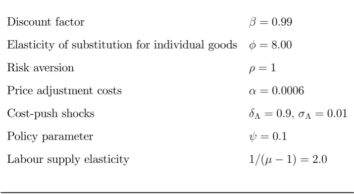
Discount factor  = 099

Elasticity of substitution for individual goods = 800

Risk aversion = 1

Price adjustment costs = 00006

Cost-push shocks Λ = 09 Λ = 001

Policy parameter = 01

Labour supply elasticity 1(₋1) = 20

Table 1: Parameter Values

benchmark case. In equilibrium (given the benchmark values for other parameters) this

implies prices are adjusted at an average rate of once every four quarters (i.e.  = 075) so

aggregate price adjustment costs are0015% of GDP in equilibrium. This total aggregate

cost is not implausibly high, given the potentially wide range of costs incorporated in

(()) but it is acknowledged that a more satisfactory basis needs to be found for

calibrating In order to test the sensitivity of the main results we consider a wide range

of alternative values for .

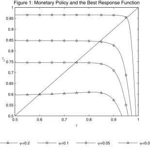
Figure 1 illustrates some of the main features of equilibrium in the benchmark case and

a number of simple variations around that benchmark case. Figure 1 plots the optimal

value of () against values of aggregate  In other words it shows the “best response

function” of firm against aggregate. The benchmark case is illustrated with the plot

marked with circles. This plot intersects the 450 _{just once. This point of intersection}

represents a single Nash equilibrium where() = _≈075

The position of the best response function, and its shape, are contingent on the values

of other parameters of the model. A change in the value of any parameter implies a

shows four other examples of best response functions - each based on a different value of

the parameter of the monetary policy rule. The higher is the more monetary policy

is aimed at stabilising the output gap, while a lower value of  implies that monetary

policy is aimed at stabilising inflation. The general pattern that emerges from the cases

illustrated in Figure 1 is that an decrease in shifts the best response function upwards,

and thus leads to an increase in the equilibrium value of  while an increase in shifts

the best response function downwards and thus leads to a reduction in the equilibrium

value of In other words, the more policy focuses on stabilisation of inflation, the lower

is equilibrium price flexibility.

The intuition behind this result is relatively straightforward. If the monetary authority

is stabilising aggregate inflation it is by definition stabilising the desired price, ˆ If the

desired price is very stable then the incentive to incur the costs of price flexibility are

much reduced, hence firms choose a high value of . At the other extreme, a high value

of  (i.e. a monetary rule which allows fluctuations in inflation in order to achieve some

stabilisation of the output gap) will necessarily cause fluctuations in the desired price,

ˆ



 This raises the incentive for firms to incur the costs of price flexibility and therefore

choose a lower value of

The results illustrated in Figure 1 correspond to the results presented by Kimura and

Kurozumi (2010). They model monetary policy in terms of a Taylor rule, rather than as

a targeting rule of the form used in this paper, but the same relationship between the

anti-inflation stance of monetary policy and the equilibrium value of  emerges. As the

feedback coefficient on inflation in the Taylor rule is increased the equilibrium value of 

increases, so output prices become lessflexible.

The cases illustrated in Figure 1 are quite regular in the sense that for each value

of  there is a single intersection between the best response function and the 450 _line,

so there is a unique Nash equilibrium. Furthermore that equilibrium is strictly within

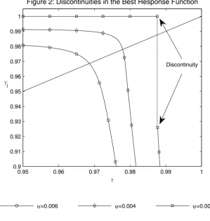
parameter becomes very small (i.e. as policy approaches strict inflation stabilisation).

Figure 2 illustrates an example of this case. Thisfigure focuses on values of very close

to zero and it shows that, for instance when= 0002there is a discontinuity in the best

response function which implies that there is no intersection with the 450 _{line. There is}

thus no simple Nash equilibrium for this (or smaller) values of9

It will become apparent below that the non-existence of a simple Nash equilibrium

for low values of  is relevant in the analysis of the welfare maximising choice of  so

it is worth considering this result in more detail. Consider the best response function

for  = 0002 shown in Figure 2. The best response function is horizontal at unity

for values of  less than approximately 0987. There is then a discrete downward jump

at  _' 0987 after which the best response function becomes downward sloping. The

discontinuity arises because the profit function is not single-peaked. Thus, for values of

in the neighbourhood of the discontinuity, the profit function has two local maxima, one

at() = 1 and one at a lower value of()For values of to the left of the discontinuity

profits are higher at () = 1 But for values of to the right of the discontinuity profits

are higher at the internal turning point in the profit function. At the discontinuity the

two maxima yield the same value of profits.

The fact that the profit function has two local maxima suggests that, even though

there is no simple Nash equilibrium with a unique equilibrium value of  there may be

a more complex Nash equilibrium where the set of firms divides into two groups, each

group setting a different value of (corresponding to the two maxima). It is considerably

more complex to derive solutions for such equilibria so we do not investigate them further

in this paper. Below, when we consider the welfare maximising choice of we therefore

confine attention to the range of values of  for which simple Nash equilibria exist (i.e.

where there is single equilibrium value).

A number of other potentially important special cases are illustrated in Figure 3, which

shows the effect of varyingthe parameter that determines the cost of price adjustment.

This figure shows that as  increases, the equilibrium value of  tends to increase. The

explanation for this is obvious. As price adjustment becomes more costlyfirms optimally

choose to make output prices less flexible.10 _{Note however that for very high values of}

 the best response function intersects the 450 line twice. There are thus two Nash

equilibria. And for the highest values of  the best response function does not intersect

with the450 _{line within the zero-one interval. In this latter case the Nash equilibrium is}

a corner solution at = 1i.e. completelyfixed prices. In other words, when the costs of

price adjustment are sufficiently high, firms optimally choose to avoid price adjustment

entirely.

Figures 2 and 3 illustrate a number of cases where the Nash equilibrium of this simple

model either does not exist, is based on a corner solution or is not unique. These cases

illustrate the benefits of working with the explicit functional form for the profit function

given by (18). By applying a numerical grid search technique to this functional form

it is possible reliably to identify the profit maximising value of () even when there

are multiple turning points in the function or when the maximum occurs at a corner.

By contrast, methods which rely on evaluating the first derivative of the profit function,

such as used by Kimura and Kurozumi (2010), potentially yield spurious results for some

parameter configurations.

10_{Notice from (18) that the profit function consists of two main terms: one that measures the expected}

profits foregone because of price inflexibility and one that measures the expected costs of price changes.

Increasing obviously increases the weight on the second term relative to the first. Notice that, other

things being equal, this is equivalent to reducing 2 _{(the variance of the innovations in the cost-push}

5

Welfare and Optimal Policy

We now consider the welfare implications of endogenous price flexibility. In particular

we consider the implications for the welfare maximising choice of the policy parameter,

 For the purposes of this exercise aggregate welfare in period 0 (i.e. at the time the

monetary policy parameter,  is set) is defined as

Ω=0

∞

X

=1

−1

½

1−

1₋ −

    ¾ (20)

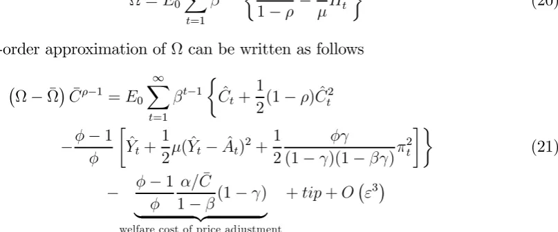
A second-order approximation ofΩ can be written as follows

¡

Ω₋Ω¯¢¯−1 =0

∞

X

=1

−1

½ ˆ

+ 1

2(1−) ˆ 2 

−−_ 1 ∙

ˆ

+ 1

2( ˆ−ˆ) 2₊1

2



(1₋)(1₋)

2 

¸¾

(21)

− −_ 1₁¯

−(1−)

| {z }

welfare cost of price adjustment

++¡3¢

Equation (21) shows that the welfare expression in this model takes the same form as in

the conventional model (with exogenous ) but with an added term that represents the

welfare costs of price adjustment.

5.1

The Benchmark Case

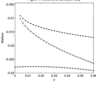
Figure 4 plots welfare against a range of values for while keeping other parameters at

their benchmark values. In this figure the plot marked with circles shows the behaviour

of welfare for the case of endogenous priceflexibility. As a point of comparison, thefigure

also shows welfare for the case where priceflexibility is exogenouslyfixed at a given level.

(This latter plot is marked with squares.) In this example we set = 075The exogenous

 case corresponds to the standard model widely analysed in the literature on optimal

monetary policy (see e.g. Benigno and Woodford (2005)) and it is therefore a natural

The welfare plot for the exogenous case shows that the welfare maximising value of

is approximately0013. This implies that it is optimal for monetary policy to allow some

volatility in inflation in order to achieve some stabilisation of the welfare-relevant output

gap. This corresponds to the result emphasised by Benigno and Woodford (2005). In

essence, cost-push shocks are distortionary and imply that the flexible price equilibrium

is sub-optimal. In a sticky price environment it is therefore not optimal for monetary

policy to reproduce theflexible price equilibrium. Sticky prices give monetary policy some

degree of leverage which can be used to stabilise output around the welfare maximising

level. This requires some volatility in inflation.

Now consider the plot of welfare in the case were priceflexibility is endogenous (i.e. the

plot marked with circles). It is immediately clear from this plot that, when priceflexibility

is endogenous, welfare appears to increase monotonically as decreases towards zero. In

other words, when price flexibility is endogenous, it appears to be optimal to engage

in aggressive inflation stabilisation. This is in contrast to the case of exogenous price

flexibility, where it is optimal to allow some variability in inflation.

As noted above (in relation to the discussion of Figure 2) in Figure 4 we confine

attention to the range of values of  for which a simple Nash equilibrium exists, i.e.

where there is a single equilibrium value ofThis implies that we do not consider values

of  below 0.0035. It is apparent from Figure 4 that this lower limit on the value of 

corresponds to the welfare maximising choice of  (within the range that we consider).

Because  does not equal zero at this point, we describe this as aggressive inflation

stabilisation rather than strict inflation targeting.

The contrast between the exogenous and endogenous flexibility cases illustrated in

Figure 4 arises for two reasons. Firstly, as is reduced, the rise in the equilibrium value

of  reduces the resource cost of priceflexibility (i.e. less frequent price changes implies

lower costs). Secondly, the rise in the equilibrium value of implies that monetary policy

on the presence of nominal rigidities and these become more significant as  increases).

Therefore, as  increases, monetary policy becomes more effective in dealing with the

distortions caused by cost-push shocks. This is reflected in a higher level of welfare as 

decreases and increases.

It is simple to measure the relative contributions of these two welfare effects by plotting

the welfare measure excluding the welfare costs of price adjustment (i.e. excluding the

term indicated in (21)) and comparing it to the full welfare measure (which includes the

costs of price adjustment). This comparison is also shown in Figure 4. The plot marked

with asterisks in Figure 4 is the value of welfare excluding the costs of price adjustment.

This can be compared to the plot marked with the circles, which shows welfare including

the costs of price adjustment. It appears that the decline in the welfare costs of price

adjustment (i.e. the vertical distance between the two plots) contributes about half of

the rise in total welfare asis reduced. The other half of the rise in welfare (i.e. the rise

in welfare illustrated in the upper plot in Figure 4) comes from the effect of more rigid

prices on the ability of monetary policy to deal with cost push shocks .

The result illustrated in Figures 4 represents a significant departure compared to the

literature based on exogenous price flexibility. That literature has emphasised that

com-plete inflation stabilisation is not optimal in the face of cost-push shocks. The comparison

between the exogenous and endogenous price flexibility cases shown in Figure 4 implies

that this basic result may be overturned when priceflexibility is endogenised.

Of course, Figure 4 is based on just one set of parameter values. Nevertheless,

exper-iments (not reported) testing the sensitivity of this basic qualitative result indicate that

it is robust across a wide range of values for key parameters, such as   and  The

basic comparison between the exogenous and endogenous price flexibility cases remains

the same across these parameter variations. Namely, it is optimal to allow some degree

of inflation variability in the exogenous price flexibility case but it is welfare enhancing

5.2

Discussion and Generalisations

As already noted, our analysis of the welfare effects of  in the endogenous  case is

restricted to values of  for which a simple Nash equilibrium exists. This places a lower

limit on the value It is apparent from the example illustrated in Figure 4 that welfare

reaches its maximum at exactly this lower limit. Our analysis therefore leaves open the

question of what happens to welfare for values of below this lower limit. This question

can only be answered by considering more complex Nash equilibria than those analysed

here. Such equilibria are likely to imply a division of the set offirms into different groups,

each with a different value of  A preliminary investigation of an example of such an

equilibrium has been carried out for the benchmark case, which suggests that welfare

continues to increase as  is reduced below the value considered in Figure 4. But a full

analysis of this type of equilibrium is well beyond the scope of this paper.

There are a number of other generalisations of our analysis which are more

straight-forward. For instance, as noted above, a more general approach to the modelling of price

adjustment costs would be to allow convexity in(), so that price adjustment is subject

to increasing marginal costs as the average frequency of price changes rises. Note that

this alternative assumption would tend to strengthen the incentive forfirms to set a high

value of . This suggests that our main result (i.e. that the optimal choice of  is very

close to zero and that the resulting equilibrium choice of byfirms is very close to unity)

is robust to convexity in the price adjustment costs function ().

The cost function could further be generalised to allow for the effects of aggregate

variables on the cost of price adjustment. For instance, the cost of price adjustment could

be assumed to fall as aggregate prices become moreflexible. An effect such as this could

easily be incorporated into our analysis.

It would also be straightforward to generalise our analysis to encompass more sources of

shocks. The results described above focus entirely on the implications of cost-push shocks.

flexibility, show that government spending shocks are very similar to cost-push shocks in

terms of their implications for optimal monetary policy. This similarity carries over into

our model. Extending our analysis to consider productivity shocks (i.e. shocks toin our

model) would also add little to the results we have emphasised above. Woodford (2003)

and Benigno and Woodford (2005), using models of exogenous priceflexibility, show that

optimal monetary policy should completely stabilise inflation in the face of productivity

shocks. In that case, our model of endogenous priceflexibility simply predicts that prices

will be completely rigid. This has no impact on the nature of optimal monetary policy in

the face of productivity shocks.

A potentially important further extension of the model would be to introduce a cost

of inflation indexation. It is well-known that the standard Calvo model generates inertia

in the price level but leaves the rate of inflation completelyflexible. Likewise, our model

makes the degree of price-level inertia endogenous while retaining the assumption that

the inflation rate is completely flexible. It has become standard in many applications

of the Calvo model to include an partial degree of inflation indexation which creates an

exogenous degree of inertia in the inflation rate. Just as the model used in this paper

endogenises the degree of price-level inertia, it would be possible to endogenise the degree

of inflation inertia by allowingfirms to choose the rate of indexation subject to some cost

of indexation. This would be another interesting line of future research.

6

Conclusion

This paper takes a standard sticky-price general equilibrium model and incorporates a

simple mechanism which endogenises the degree of nominal priceflexibility. The analysis

shows that the equilibrium degree of price flexibility is sensitive to changes in monetary

policy. For instance, the more the more weight monetary policy places on inflation

flexibility tends to shift optimal monetary policy towards complete inflation stabilisation,

even when shocks take the form of cost-push disturbances. This contrasts with the

stan-dard result obtained in models with exogenous price flexibility, which show that optimal

monetary policy should allow some degree of inflation volatility in order to stabilise the

welfare-relevant output gap.

The model we develop and analyse in this paper takes a somewhat stylised shortcut to

the representation of endogenous priceflexibility. A more theoretically appealing approach

would be to develop a structural model of state-dependent price setting. While such

models are being developed and analysed in the recent literature, they are still some

way from being tractable enough to allow a detailed analysis of optimal monetary policy.

In lieu of further progress with the development of state-dependent pricing models, the

results we present in this paper offer a potentially useful benchmark for judging the impact

of endogenous priceflexibility on the welfare effects of monetary policy.

Acknowledgements

We are grateful to two anonymous referees for many useful comments on an earlier draft

References

Ascari, G. and L. Rossi (2012) “Trend Inflation and Firms’ Price Setting: Rotemberg

versus Calvo”Economic Journal, 122, 1115-1141.

Benigno, P. and M. Woodford (2005) “Inflation Stabilization and Welfare: The Case of a

Distorted Steady State”Journal of the European Economic Association,3, 1185-1236.

Calmfors, L. and A. Johansson (2006) “Nominal Wage Flexibility, Wage Indexation, and

Monetary Union” Economic Journal,116, 283-308.

Calvo, G. A. (1983) “Staggered Prices in a Utility-Maximising Framework” Journal of

Monetary Economics, 12, 383-398.

Devereux, M. B. (2006) “Exchange Rate Policy and Endogenous Price Flexibility”,

Jour-nal of the European Economic Association, 4, 735—769.

Devereux, M. B. and H. E. Siu (2007) “State Dependent Pricing and Business Cycle

Asymmetries”International Economic Review, 48, 281-310.

Devereux, M. B. and J. Yetman (2002) “Menu Costs and the Long Run Output-Inflation

Trade-off” Economic Letters, 76, 95-100.

Devereux, M. B. and J. Yetman (2003)“Price-Setting and Exchange Rate Pass-Through:

Theory and Evidence” in Price Adjustment and Monetary Policy: Proceedings of a

Conference Held by the Bank of Canada, Bank of Canada Publications, Ottawa,

347-371.

Devereux, M. B. and J. Yetman (2010)“Price Adjustment and Exchange Rate

Pass-through” Journal of International Money and Finance, 29, 181-200.

Dotsey, M. and R. G. King (2005) “Implications of State-Dependent Pricing for Dynamic

Dotsey, M., R. G. King and A. L. Wolman (1999) “State Dependent Pricing and the

Gen-eral Equilibrium Dynamics of Money and Output” Quarterly Journal of Economics,

114, 655-690.

Golosov, M. and R. E. Lucas (2007) “Menu Costs and Phillips Curves” Journal of

Political Economy, 115, 171-199.

Ho, A. W. Y. and J. Yetman (2008) “The Long-Run Output-Inflation Trade-off with

Menu Costs”North American Journal of Economics and Finance, 19, 261-273.

Kimura, T. and T. Kurozumi (2010) “Endogenous Nominal Rigidities and Monetary

Policy” Journal of Monetary Economics, 57, 1038-1048.

Kimura, T., T. Kurozumi and N. Hara (2008) “Endogenous Nominal Rigidities and

Monetary Policy” Bank of Japan, Tokyo, unpublished manuscript.

Kiley, M. T. (2000) “Endogenous Price Stickiness and Business Cycle Persistence”

Jour-nal of Money, Credit and Banking, 32, 28-53.

Levin, A. and T. Yun (2007) “Reconsidering the Natural Rate Hypothesis in a New

Keynesian Framework”Journal of Monetary Economics, 54, 1344-1365.

Romer, D. (1990) “Staggered Price Setting with Endogenous Frequency of Adjustment”

Economics Letters, 32, 205-210.

Rotemberg, J. J. (1982) “Monopolistic Price Adjustment and Aggregate Output”Review

of Economic Studies, 49, 517-531.

Senay, O. and A. Sutherland (2006) “Can Endogenous Changes on Price Flexibility Alter

the Relative Welfare Performance of Exchange Rate Regimes?” inNBER International

Seminar on Macroeconomics 2004 R. H. Clarida, J. F. Frankel, F. Giavazzi and K.

Woodford, M. (2003) Interest and Prices: Foundations of a Theory of Monetary Policy

Princeton University Press, Princeton, NJ.

Yetman, J. (2003) “Fixed Prices versus Predetermined Prices and the Equilibrium

Appendix

Optimal Prices and Aggregate Inflation

Expressions (13) and (14) are derived using (3), (7) and (11). The coefficients Λ, Λ

and are given by the following

Λ=ΓΛ(1−Λ) =Γ(1−) Λ =ΓΛ 

 =Γ 

 (22)

where

ΓΛ =

[1 +Λ] +(1₋Λ)

 Γ=−

[1 +]

+(1₋) (23)

Approximation of Firm ’s Expected Profit Function

A second-order approximation of (15) is derived as follows. First substitute for()and

rearrange to yield

Π() = 1

_− ∞ X = − " 1 µ ()  ¶1−

−2 µ

()

 ¶−

−_−(1₋())

 #

(24)

where

1 =− and2 =−Λ





−_1 (25)

This form of the profit function isolates terms which depend on () A second order

approximation implies

˜

Π0()−Π¯ = −

(₋1)

2 ¯ 0

∞

X

=1

−1h(ˆ()₋ˆ)2 ₋2(ˆ2−ˆ1)(ˆ()−ˆ) i

−−_ 1₁ 

−(1−()) ++

¡

3¢ (26)

whererepresents terms independent offirm. This may be written in the form of (16)

by noting that

ˆ

2−ˆ1 = ˆΛ+ ˆ−ˆ−ˆ+ ¡

The Expected Dynamics of Firm ’s Price

The first-order condition for price setting forfirm implies

ˆ

()₋ˆ= (1−())(ˆ−ˆ) +()[ˆ+1()−ˆ+1] +()[+1] + ¡

2¢ (28)

When combined with (13) and (14) it is simple to show thatˆ()₋ˆ can be written in

the form

ˆ

()₋ˆ=ΛΛˆ+ˆ+ ¡

2¢ (29)

where Λ and are given by

Λ = ΓΛ

(1₋Λ)(1−())+Λ()

(1₋Λ())

(30)

 = Γ

(1₋)(1₋())+()

(1−())

(31)

To complete the solution for 0[(ˆ −ˆ)(ˆ()−ˆ)] and 0[(ˆ()−ˆ)2] it is

use-ful to decompose the expectations operator 0 into 0 expectations across aggregate

disturbances, and 

0 expectations across the Calvo pricing signal for firm , where

0[] = 

0 [0[]] (Note that 0[] is conditional on particular realised values of the

aggregate disturbances,Λˆandˆ.) Since aggregate disturbances and aggregate variables

are independent from the Calvo pricing signal forfirm, we may write

0[(ˆ−ˆ)(ˆ()−ˆ)] =   0 [(ˆ



 −ˆ) 

0 [ˆ()−ˆ]] (32)

It is thus necessary to obtain a first-order accurate solution for 

0 [ˆ()−ˆ]

The Calvo pricing process implies that 0[ˆ()−ˆ] evolves according to

₀[ˆ()₋ˆ] =()₀[ˆ−1()−ˆ−1] + (1−())(ˆ()−ˆ)−()+ ¡

2¢ (33)

This can be solved and combined with (13) and (17) to yield a second-order accurate

expression for0[(ˆ

 −ˆ)(ˆ()−ˆ)]

An equation for the evolution of 0[(ˆ()₋ˆ)2_{]can be derived in a similar way. The}

Calvo pricing process implies that

0[(ˆ()₋ˆ)2] =()0[(ˆ−1()−ˆ)2] + (1−())0[(ˆ()−ˆ)2] +

¡

Using the relationships

0[(ˆ−1()−ˆ)2] =0[(ˆ−1()−ˆ−1)2] +0[2]−20[(ˆ−1()−ˆ−1)] (35)

0[(ˆ−1()−ˆ−1)] =0[0(ˆ−1()−ˆ−1)] (36)

equation (34) can be written as

0[(ˆ()₋ˆ)2] = ()0[(ˆ−1()−ˆ−1)2] + (1−())0[(ˆ()−ˆ)2]

+()0[2_]₋2()₀[0(ˆ−1()−ˆ−1)] +

¡

3¢ (37)

which can be solved in combination with (13) and (17) to yield a second-order accurate

0.5 0.6 0.7 0.8 0.9 1 0.5

0.55 0.6 0.65 0.7 0.75 0.8 0.85 0.9 0.95

1Figure 1: Monetary Policy and the Best Response Function

 _j

0.95 0.96 0.97 0.98 0.99 1 0.9

0.91 0.92 0.93 0.94 0.95 0.96 0.97 0.98 0.99 1

Figure 2: Discontinuities in the Best Response Function

 _j

=0.006 =0.004 =0.002

0.5 0.6 0.7 0.8 0.9 1 0.5

0.55 0.6 0.65 0.7 0.75 0.8 0.85 0.9 0.95 1

Figure 3: Price Adjustment Costs and the Best Response Function

 _j

0 0.01 0.02 0.03 0.04 0.05 0.06 -0.03

-0.025 -0.02 -0.015 -0.01 -0.005

Figure 4: Welfare and Monetary Policy

Welfare

