A review of thermal and optical characterisation of complex window systems and their building performance prediction

1

A Review of Thermal and Optical Characterisation of Complex

Window Systems and Their Building Performance Prediction

Yanyi Sun, Yupeng Wu* and Robin Wilson

Department of Architecture and Built Environment, Faculty of Engineering, The University of Nottingham, University Park, Nottingham, NG7 2RD, UK

*Corresponding author: Tel: +44 (0) 115 74 84011; emails: [email protected], [email protected]

Abstract:

Window systems play a key role in establishing both the thermal and luminous environments within buildings, as well as the consequent energy required to maintain these for the comfort of their occupants. Various strategies have been employed to improve the thermal and optical performance of window systems. Some of these approaches result in products with relatively complex structures. Thus, it becomes difficult to characterise their optical and thermal properties for use in building performance prediction. This review discusses the experimental and numerical methods used to predict the thermal and optical behaviour of complex window systems. Following a discussion of thermal characterisation methods available in the literature that include experimental test methods, theoretical calculation methods and Computational Fluid Dynamic methods, sophisticated optical methods, such as use of Bidirectional Scatter Distribution Functions (BSDF) to optically characterise complex window systems, are introduced. The application of BSDF allows advanced daylight assessment metrics along with daylight evaluation tools to be used to realise dynamic annual prediction of the luminous environment. Finally, this paper reviews methods that permit the prediction of the combined thermal, daylight and energy behaviour of buildings that make use of complex window systems.

Keywords:

2 Nomenclature

Symbols

𝑐_𝑝 specific heat capacity J/kgK 𝑣 kinematic viscosity m2_/s

𝐶𝑜𝑛𝑠𝑡. constant - V(λ) spectral luminous efficiency

for photonic vision

-

𝑑 thickness of glass pane m

Dλ spectral distribution - 𝑥, 𝑦 Cartesian coordinates -

e exponent - ∆𝑇 temperature difference K

Ev vertical eye illuminance lux ∆𝜆 wavelength interval nm

Eo exterior IR incident on window plane

W/m2 _{𝛽 thermal expansion coefficient 1/K}

𝜀 Emissivity -

Ei interior IR incident on window plane

W/m2 _{𝜎 Stefan-Boltzmann constant W/m}2_K4

θ incidence angle °

𝐹 view factor - φ azimuth angle °

𝑔 gravitational acceleration m/s2 _{λ wavelength nm}

ℎ heat transfer coefficient W/m2_K τ _{transmittance}

-- also thermal conductance W/m2_{K 𝜇 dynamic viscosity of gas kg/ms}

𝐽 radiosity W/m2 _{𝜌 density of air kg/m}3

𝑘 thermal conductivity W/mK 𝜔𝑠 solid angle sr

Ls luminance of source cd/m2

N number - 𝐃𝐢𝐦𝐞𝐧𝐬𝐢𝐨𝐧𝐥𝐞𝐬𝐬 𝐍𝐮𝐦𝐛𝐞𝐫𝐬

𝑝 pressure Pa Gr Grashof number

P position index - Nu Nusselt number

𝑞 heat flux W/m2 _{Pr Prandtl number}

𝑅 thermal resistance mK/W

𝑠 thickness of the window air cavity

m Subscripts

e external

Sh radiative heat transfer g gas

Si radiation (short-wave, and long-wave from zone internal sources) absorbed by face i

W/m2 _{p glass pane}

H hot i internal i, j, k counter

𝑇 temperature ℃ m mean

𝑈 thermal transmittance W/ m2_{K t total}

𝑢, 𝑣 velocity components r radiation

1.

Introduction

Windows in building envelopes are critical components that determine direct solar energy gains and daylight, facilitate the view into and out of a building, and influence overall building energy consumption [1-3]. However, the material properties of glass when used in conventional windows arouse concerns in response to the recent sustainability agenda, in particular in relation to the responsible use of energy in buildings. The most common issues are:

3

2) Significant heat loss during cold seasons due to the relatively high U-value compared with walls or ceilings [7-12];

3) Visual discomfort from glare in work spaces [13-15];

4) Glare caused by the reflection of sunlight from glazing to a buildings immediate surroundings or the city more widely [16];

5) Air infiltration through defects between glazing and frame due to poor workmanship [17, 18];

6) Degradation and fading of building components or furniture due to the presence of high levels of transmitted sunlight in the internal environment [19, 20].

Improvements to the design and manufacture of window systems seek to optimise the effective use of solar resource, minimise undesired energy losses and effectively moderate the indoor environment. The two main strategies that have been applied are: 1) increasing thermal resistance using approaches such as multiple glass panes, inert gases as cavity fill, low emissivity coatings, and vacuum glazing; 2) controlling solar radiation and daylight through application of tinted coatings, reflective coatings, interstitial shading devices, and smart window techniques (e.g. electrochromic, thermochromic, photochromic glazing). Some of these approaches result in window systems with relatively complex structures, which increases the challenge of accurately characterising their behaviour for use in studies of building performance. The process of characterisation for these complex glazing systems involves investigations that explore and quantify both their thermal and optical behaviours. There is little in the literature, however, that reviews these methods of characterisation or explores their use to inform the predicted performance of buildings employing these systems. This review will play a critical role in addressing these challenges and suggest ways in which they might be used to inform the future application of novel and complex window systems to buildings.

4

that permit the prediction of the combined thermal, daylight and energy behaviour of spaces served by complex window systems.

2.

Thermal investigations of window systems

In this section, the experimental and numerical methods that can be used to evaluate the thermal properties of a building component, with a focus on window systems with complex structures, is introduced and discussed.

2.1Experimental investigation methods

5

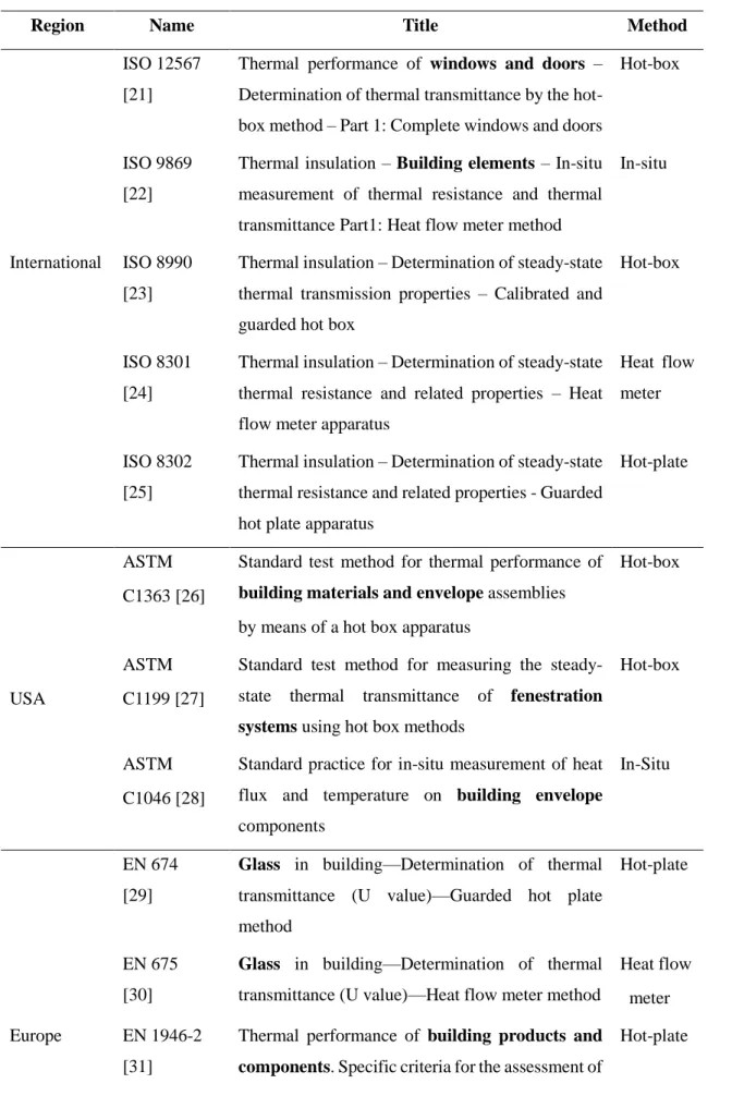
Table 1: Standards for determining thermal properties using experimental methods

Region Name Title Method

ISO 12567

[21]

Thermal performance of windows and doors – Determination of thermal transmittance by the hot-box method – Part 1: Complete windows and doors

Hot-box

ISO 9869 [22]

Thermal insulation – Building elements – In-situ

measurement of thermal resistance and thermal transmittance Part1: Heat flow meter method

In-situ

International ISO 8990 [23]

Thermal insulation – Determination of steady-state

thermal transmission properties – Calibrated and guarded hot box

Hot-box

ISO 8301

[24]

Thermal insulation – Determination of steady-state

thermal resistance and related properties – Heat flow meter apparatus

Heat flow

meter

ISO 8302 [25]

Thermal insulation – Determination of steady-state thermal resistance and related properties - Guarded

hot plate apparatus

Hot-plate

ASTM

C1363 [26]

Standard test method for thermal performance of

building materials and envelope assemblies

by means of a hot box apparatus

Hot-box

USA

ASTM

C1199 [27]

Standard test method for measuring the

steady-state thermal transmittance of fenestration systems using hot box methods

Hot-box

ASTM

C1046 [28]

Standard practice for in-situ measurement of heat flux and temperature on building envelope

components

In-Situ

EN 674 [29]

Glass in building—Determination of thermal transmittance (U value)—Guarded hot plate

method

Hot-plate

EN 675

[30]

Glass in building—Determination of thermal transmittance (U value)—Heat flow meter method

Heat flow

meter

Europe EN 1946-2

[31]

Thermal performance of building products and components. Specific criteria for the assessment of

6

laboratories measuring heat transfer properties. Measurements by guarded hot plate method

EN 1946-3 [32]

Thermal performance of building products and components – Specific criteria for the assessment of laboratories measuring heat transfer properties—Part 3: Measurements by heat flow

meter method

Heat flow meter

Russian GOST

26602.1 [33]

Windows and doors. Methods of determination of resistance of thermal transmission

Hot-box

7

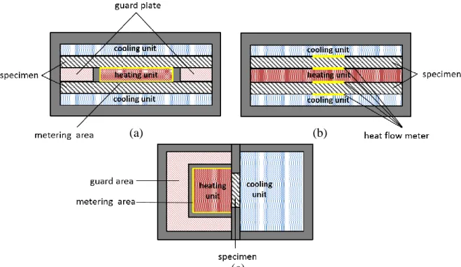
Figure 1: Steady-state thermal properties laboratory measurement method (a) hot-plate method, (b) flow meter

method and (c) hot-box method

The hot-plate and flow meter methods are suited for characterising homogeneous materials, such as single glazing, insulation materials, etc. Goetzberger [34], Platzer [35, 36] and Suehrcke et al. [37] used hot-plate methods to measure the thermal characteristics of various Transparent Insulation Materials (TIMs). When faced with the issue of measuring the overall heat transfer through large, inhomogeneous structures, such as glazing with frames or shading devices, the hot-box method [21, 23, 26, 27, 33] is better suited and more widely used [38]. In this apparatus (Figure 1 (c)), the specimen is mounted between two chambers that are kept at stable hot and cold conditions. The hot chamber serves as a guard to a metering box, which is mounted over the test sample. By maintaining equal temperatures in the hot chamber and the metering box, all the heat supplied to the metering box is assumed to be transmitted through the sample, which is then be used to determine the thermal transmittance of the sample [39]. Asdrubali and Baldinelli [40] compared three hot-box methods according to ISO 8990 [23], ASTM C1363 [26] and GOST 26602.1 [33] respectively. The results revealed that ISO 8990 and ASTM C1363 are very similar since they only measured the total heat transfer through the specimen; while GOST 26602.1 measured individual thermal characteristics of each component of the specimen, giving more information on the weaknesses and strengths of these components.

The method to obtain the dynamic thermal properties of building components uses thermocouples and heat flux meters to measure both the temperature gradient between any

(a) (b)

8

two surfaces of a building component, as well as the heat transfer rate through them, on the site where they are situated [22, 28]. There are, however, various factors that can significantly affect the accuracy of the measurements taken. These include the type and quantity of sensors used, component location, and extreme ambient conditions. There are also some challenges that cannot easily be controlled during a measurement, such as seasonal weather, wind speed and radiant energy from the sun, which can make measurements impractical [41, 42].

2.2Numerical investigation methods

The numerical investigation of the thermal properties of window systems can be classified into two major groups: 1) one-dimensional calculation based on standard calculation methods and 2) two- or three-dimensional simulation using finite element or finite volume models.

2.2.1 Standard calculation method

Standards describing the centre-of-glazing thermal behaviour of window systems include International Standards ISO 10292 [43] and ISO 15099 [44] and European Standard EN 673 [45].

Under these standards, the centre-of-glazing U-value, which is the reciprocal of total thermal resistance consisting of the internal and external surface thermal resistances and the thermal resistance of the glazing unit, can be described by the following equation:

𝑈 = 1

𝑅_𝑡=

1 1

ℎ_𝑒+ 𝑅 +ℎ1_𝑖

(1)

where, he and hi are the external and internal heat transfer coefficients, respectively. For a vertical soda lime glass surface, the value of he used in standard EN 673 [45] is 25 W/m2K and the value of hi is 7.7 W/m2K. These two values are standardised for the purposes of comparing glazing U-values. The total thermal resistance of the glazing unit, R, can be described for double glazing using the following equation [45]:

𝑅 = 1

ℎ_𝑟+ ℎ_𝑔+ 2 𝑑

𝑘_𝑝 (2)

9

According to the empirical equation provided in EN673 [44], the radiation conductance, hr, is given by:

ℎ_𝑟 = 4𝜎 (1 𝜀1+

1 𝜀2− 1)

−1

𝑇_𝑚3 ₍₃₎

where σ is the Stefan-Boltzmann’s constant, Tm is the mean absolute temperature of the gas space, 1 and 2are the corrected emissivities of the surfaces bounding the enclosed space between the panes at temperature, Tm. For uncoated soda lime glass surfaces, 0.83 can be used as the corrected emissivity [45], while the corrected emissivity for a glass surface with low-emissivity coating can be as low as 0.013 [46].

The thermal conductance of the gas in the cavity is given by:

ℎ𝑔 = 𝑁𝑢

𝑘_𝑔

𝑠 (4)

where s is the thickness of the air cavity, kg is the thermal conductivity of the air space. The

Nusselt number, Nu, which indicates the intensity of convection by representing the ratio between the pure conduction resistances to a convection resistance [32], is given by:

𝑁𝑢 = 𝐶𝑜𝑛𝑠𝑡. (𝐺𝑟 ∙ 𝑃𝑟)𝑒 ₍₅₎

where Const. is a constant and e is an exponent that makes it possible to account for the orientation of the glazing. For vertical glazing, these are 0.035 and 0.38 respectively [44]. The Grashof number, Gr, and the Prandtl number, Pr, are given by:

𝐺𝑟 =𝑔𝛽∆𝑇𝑠3

𝑣2 (6)

and

𝑃𝑟 = 𝑐𝑝𝜇

𝑘_𝑔 (7)

10 2.2.2 Numerical models

Apart from experimental measurement and standard equation calculation methods, finite element or finite volume simulations are the most common approach used in order to obtain the thermal properties of window systems, especially when the air flow pattern in the cavity is of particular interest.

Computational Fluid Dynamics (CFD) tools have been used by researchers to solve the heat transfer problem and explore the air flow pattern in the vertical air cavity of both conventional double glazed units [52-56] and complex window systems [7, 57-61] .Zhao et al.[52] Wright et al. [54] and Ganguli et al. [55, 56] used a finite volume method to study natural convection in the cavity of double glazed units. The possibility of reducing free convection by integrating shading devices, such as horizontal Venetian blinds, pleated blinds and different configurations of fins into the cavity of double glazed units has also been investigated [7, 57-61]. In their finite volume models, the following assumptions were made: 1) the glass surfaces facing into the cavity were set as two isothermal walls each with a different temperature to represent the temperature difference between indoor and outdoor environments; 2) the top and bottom surfaces bounding the cavity were assumed to be adiabatic; 3) the cavity was filled with air with a Prandtl number of approximately 0.71

[57-61]. All thermophysical properties of the fluid were assumed to be constant, except for the fluid

density and viscosity [57-61] .

The governing equations for these finite volume models are [57-61]:

Mass balance:

∂u ∂x+

𝜕𝑣

𝜕𝑦= 0 (8)

Momentum balance:

ρ (u∂𝑢 ∂𝑥+ v

𝜕𝑢 𝜕𝑦) = −

∂p ∂x+ 𝜇 (

∂2_𝑢

𝜕𝑥2+

∂2_𝑢

11 𝜌 (u∂v

∂x+ v 𝜕𝑣 𝜕𝑦) = −

∂p ∂x+ 𝜇 (

∂2_𝑣

𝜕𝑥2+

∂2_𝑣

𝜕𝑦2) + 𝜌𝑔𝛽(𝑇 − 𝑇𝐶) (10)

Energy balance:

𝜌𝑐_𝑝(𝑢𝜕𝑇 𝜕𝑥+ 𝑣

𝜕𝑇

𝜕𝑦) = 𝑘 ( ∂2_𝑇

𝜕𝑥2+

∂2_𝑇

𝜕𝑦2) (+𝑆ℎ) (11)

However, in most of these studies, long-wave radiation heat transfer, which accounts for two thirds of the total heat transfer across the air cavity [53], is neglected in the numerical modelling, which means the radiative heat transfer, Sh in Equation (11), was not included. Some improved simulation methods have been implemented by Avedissian and Naylor [58] and Sun et al. [61], who used a “surface-to-surface” (S2S) model to include radiation. All the surfaces were assumed to be grey bodies, diffuse and opaque to thermal radiation. The air in the cavity was assumed to be a non-participating medium. The view factors (Fkj), which depend on surfaces’ size, separation distance and orientation, were computed before simulating the radiation. The S2S method can be represented by the following equation:

𝐽𝑘 = 𝜀𝑘𝜎𝑇𝑘4 + (1 − 𝜀𝑘) ∑𝑁𝑗=1𝐹𝑘𝑗𝐽𝑗 (12)

Through CFD simulation, the convective heat flux and combined convective and radiative heat flux at the boundaries of the two glazing panes can be obtained from the converged temperature field. The overall thermal conductance (h) including both radiation conductance between two glass panes and the thermal conductance of air cavity of a double glazing unit with or without a complex interstitial structure can be expressed in Equation (13):

ℎ =(

𝜕𝑇 𝜕𝑥)𝑝 𝑘𝑎

∆𝑇 =

𝑞

∆𝑇 (13)

12

The Nusselt number of convective heat flux, which is determined by empirical equation in standard calculation method, can also be expressed by the calculated air temperature gradient using Equation (14):

𝑁𝑢 =(

𝜕𝑇 𝜕𝑥)𝑝 𝑠

∆𝑇 =

𝑞′𝑠

𝑘_𝑎∆𝑇 (14)

where q’(W/m2) is the average convective heat flux across the two surfaces.

Some of these models have been validated by temperature field visualisation obtained by interferometry [62-64], while other models have been validated by hot-box tests [65].

3.

Optical investigations of complex window systems

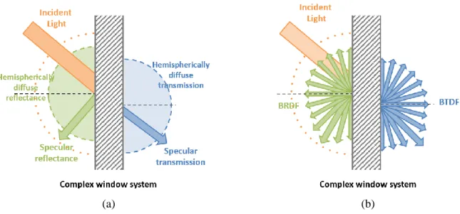
There are two primary ways of expressing the optical properties of a window system containing a complex structure (e.g. interstitial shading devices) as illustrated in Figure 2. The first quantifies the strength and direction of the direct flux and then quantifies the remaining flux as a single value by assuming it is diffuse and contains no useful directional information. These data, describing the total amount of transmitted/reflected flux, are sufficient for predicting solar gains in cases where directional information is not important. The second is to use a method such as Bidirectional Scattering Distribution Functions (BSDF), which represent magnitude and the directional qualities of reflected or transmitted flux.

Figure 2: Methods for qualifying the transmission/reflection behaviour of glazing systems: (a) Simple: diffuse

component expressed as an angular coverage value; (b) Complex: specular and diffuse components discretised and

expressed as vectors.

(a) (b)

13

If there is a requirement to retain information relating to the direction of entry of the light to its direction(s) of exit, as the case of daylight distribution calculations, these more sophisticated measure measures of glazing behaviour are required.

The following two sections introduce experimental methods (i.e. spectrophotometer combined with integrating sphere measurements or goniophotometer measurements) and numerical methods (i.e. radiosity or ray-tracing) to obtain these two types of measure.

3.1Simple methods to measure total transmittance or reflectance

The measurement of transmittance and reflectance of a building component can be obtained using a spectrophotometer and an integrating sphere. International Standard ISO 9050 [66] and European Standard EN410 [67] describe the methods used to calculate light and solar transmittance/reflectance based on the measured spectral transmittance/reflectance data. The technical requirements of the measurement apparatus and details of their use to determine these quantities are described in International Commission on Illumination (CIE) standard [68]. A schematic of the experimental setup is shown in Figure 3 [69].

Figure 3: Experiment set up for measuring transmittance and reflectance (adopted from [69]): (a)

overview of apparatuses; (b) use of integrating sphere/ spectrometer to qualify transmitted (T) and

reflected (R) components.

As shown in Figure 3 (b), the integrating sphere is used to detect the diffuse and the total magnitude of transmittance, Tdiffand Ttotal respectively [69]. The diffuse transmittance is obtained by opening a port and letting the specular component exit the integrator. The

(a)

14

specular transmitted component, Tspec is determined from the difference, Ttotal-Tdiff [69]. The same approaches are adopted in determining reflected qualities.

Photometric data can be obtained based on the measurement of light transmittance over a number of wavelength intervals in the visible wavelength range (380 ~ 780 nm). From these, the overall light transmittance, 𝜏_𝑣, of a glazing component can be calculated using the following equation [67]:

𝜏𝑣 = ∑ 𝐷𝜆

780

380 𝜏(𝜆)𝑉(𝜆)𝛥𝜆

∑780380𝐷𝜆𝑉(𝜆)𝛥𝜆 (15) where Dλ is the relative spectral distribution of light source (e.g. illuminant D65); τ(λ) is the

spectral transmittance of the glazing over wavelength interval 𝛥𝜆, and V(λ) is the spectral luminous efficiency for photonic vision defining the standard observer. The solar transmittance is obtained by neglecting the V(λ) correction and is typically determined over the wavelength range from 300 nm to 2500 nm [67].

A singnificant volume of research refers to this methodology in relation to the exploration of innovative glazing materials and window systems in terms of their respective optical prefromance [70-77]. However, this method of combining a spectrophotometer with an integrating sphere is mainly suited to the characterisation of homogenous glazing systems or materials. In the case of a window system that includes a complex interstitial structure, the standard integrating sphere measurement method can prove inappropriate as it does not easily accommodate the effects of anisotropy and spatial variation that are typically present. These can result in significant deviation in the directional characteristics of transmitted and reflected flux as well as variation in the total amount of flux transmitted/reflected. Not only can this give rise to significant errors in the estimates of transmission, these simple methods of measurement do not capture valuable directional information that is necessary to make accurate predictions of daylight distribution in the room served by these glazing systems.

3.2Numerical methods for predicting total transmittance or reflectance

15

patch is considered as a Lambertian reflector [78] and the view factors between all patches are paired in an iterative calculation [79]. When the beam radiation passes through the structure without intercepting any of the slats (Figure 4 (b)), it is regarded as contributing to the direct transmittance, 𝜏_{𝑑𝑖𝑟, 𝑑𝑖𝑟}. When either the beam radiation or incident diffuse radiation intercepts the slats, it is regarded as contributing to the spatially averaged diffuse transmittance or reflectance, which may be broken down into sub components i.e. direct-to-diffuse (𝜏_{𝑑𝑖𝑟, 𝑑𝑖𝑓}, 𝜌_{𝑑𝑖𝑟, 𝑑𝑖𝑓}) and diffuse-to-diffuse (𝜏_{𝑑𝑖𝑓, 𝑑𝑖𝑓}, 𝜌_{𝑑𝑖𝑓, 𝑑𝑖𝑓}) as shown in Figure 3 (c, d) [44].

Figure 4: (a) discretisation used to model a Venetian blind, (b) the direct-direct transmittance of the shading device,

(c) the direct-diffuse transmittance and reflectance of the shading device and (d) illustration of the diffuse-diffuse

transmittance and reflectance of the shading device [44]

The radiosity method as described in ISO15099 has been utilised in building simulation software, such as EnergyPlus, to calculate the transmittance and reflectance of a window system with complex interstitial structures [79]. Its application to window systems with integrated Venetian blinds has been implemented by a number of investigators [80-88] and has proved to be a quick and effective numerical method. The assumption of Lambertian surfaces means that this method is not suitable for systems with highly specular surfaces, however, overcome this limitation, researchers [89-91] have proposed a mixed method that combines radiosity with a ray-tracing method to yield both the specular and scattering optical characteristics.

This approach can yield simple averaged optical properties, however, when the application requires the outgoing directions of light to predict its distribution in a space, knowledge of only the ratio between the amounts of transmitted or reflected light to the

16

amount of incident light is no longer sufficient. A detailed knowledge of directional optical properties is necessary.

3.3Complex methods for determining transmittance and reflectance –

the Bidirectional Scattering Distribution Function (BSDF)

The Bidirectional Scattering Distribution Function (BSDF) comprises matrices of coefficients that for light from each incident direction quantify the proportion transmitted in each outgoing direction. It is currently regarded as the most important method for characterising complex glazing systems, allowing them to be represented with precision in daylight analysis simulations. The BSDF can be further divided into a Bidirectional Transmittance Distribution Function (BTDF) and a Bidirectional Reflectance Distribution Function (BRDF). The BSDF based on Klems’ angle basis (Figure 5 (a) ) [92, 93] is the most commonly used format. It is formed by 145 x 145 matrices including both solar and optical spectrum. Each matrix describes reflectance or transmittance distribution in the outgoing hemisphere for a single incidence angle from the incoming hemisphere. Equation (9) [94] illustrates how the value of total transmitted radiation is obtained with regard to any particular angle of incidence (azimuth, θ1 and altitude, φ1). This value is derived using a matrix calculation based on the result of the sum of the individual products of the luminous coefficients and incident irradiance, for each segment of the hemispherical basis.

τ(θ₁, φ₁) = ∑ BTDF(patch_k) ∫ dφ₂∫ cos θ₂sin θ₂dθ₂ (16)

π/2

0 2π

0 145

k=1

where, θ and φdefine the boundaries of each patch as shown in Figure 5(b).

17

Figure 5: (a) Klems’ 145-patch hemispherical basis with numbered subdivisions; (b) coordinate system for

bidirectional measurements [94]

Recent investigators have focused on the development of measurement techniques for complex window systems in an attempt to capture the respective BRDF and BTDF data. The instrument most commonly used is a goniophotometer and these can be divided into two catalogues: 1) scanning-based instruments, where each outgoing direction of light is detected by each individual movement of the detector, and 2) video-based instruments, where digital imaging techniques are used to collect the outgoing direction of light from a single image. The schematic diagrams and features of goniophotometers are illustrated in Table 1.

As suggested by the name, the scanning-based method measures all required incoming and outgoing light flux directions by moving the sample, detector or light source. Each value in the BSDF matrix is measured discretely. Although, this method is intuitive and can offer high and variable angle resolution [69], it is an onerous time consuming task (i.e. 4 to 30 days according to [95]). Moreover, the scanning of discrete BSDF-related data presents the potential risk of omitting significant features that may lie between the points where measurement are taken [69, 95].

18

Table 2: Goniophtotometers to measure the BSDF data

Institute LBNL, USA ISE, Germany Cardiff University, UK pab Ltd, Germany

Schematic

Method Scanning-based Scanning-based Scanning-based Scanning-based

Year 1988 1994 2001 2006

BTDF √ √ √ √

BRDF - √ - √

Spectral

capability

- - √ -

Validated

by

measured g-value transmittance measured with integrating

sphere

measured g-value, transmittance measured with

integrating sphere

-

19

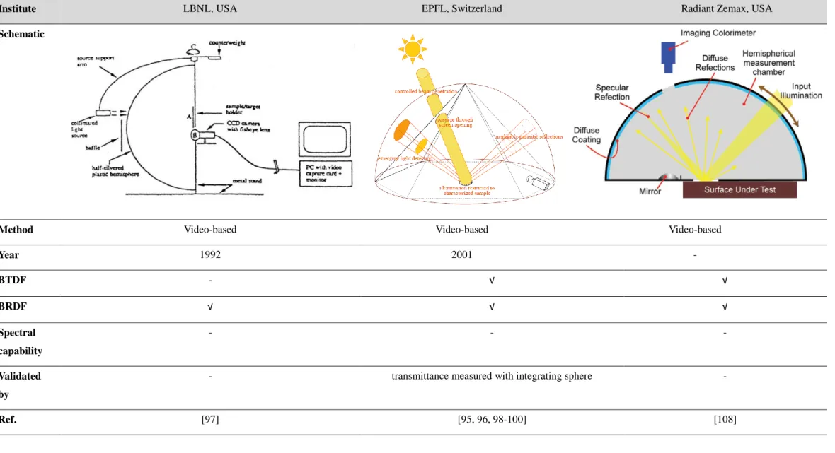
Table 3: Goniophtotometers to measure the BSDF data (continued)

Institute LBNL, USA EPFL, Switzerland Radiant Zemax, USA

Schematic

Method Video-based Video-based Video-based

Year 1992 2001 -

BTDF - √ √

BRDF √ √ √

Spectral

capability

- - -

Validated

by

- transmittance measured with integrating sphere -

20

The complexity and the levels of skill required to operate goniophotometers means that they have received relatively low levels of uptake in both academic and commercial sectors.

As an alternative, researchers have been developing and validating virtual goniophotometers based on commercial forward ray-tracing simulation tools and using these in conjunction with virtual representations of complex fenestration systems (based on description of their geometry and optical characteristics) to obtain BSDF data. This approach is easier to implement, less expensive, less time-intense and more flexible for conducting parametric studies. Researchers in LESO-PB/EPFL [98, 99] used commercial ray-tracing software TracePro to model a virtual goniphotometer, which has same configuration (i.e. receiving surfaces that consist of six triangles) as the experimental goniophotometer in EPFL, as shown in Figure 6 (a). The results were validated by comparison with experimental data and showed a difference of between 2 ~14%. Another numerical goniophotometer was developed by de Boer [109] using the ray-tracing tool OptiCad, as shown in Figure 6 (b). This method used virtual sensors to receive flux on individual geometric positions and then calculated the BSDF values. The resolution of this numerical goniophotmeter can be defined by the user [95].

21

Figure 6: Virtual goniophotometers generated using (a)TracePro [98] and (b)OptiCad [109]

22

4.

Daylight performance predictions for buildings with complex

fenestration systems

The quantity, quality and distribution of natural daylight passing through window systems and illumination of an interior space, play an important role in determining building energy efficiency and indoor environmental quality [113]. For example, excess sunlight in summer results in unwanted glare and presents an overheating risk, insufficient daylight results higher electricity consumption due to the use of artificial lighting, etc. Additionally, appropriate provision of daylight is also proven to have beneficial effects on human health, mood, activity and working efficiency [114].

Traditional approaches to evaluating the quantity, quality and distribution of daylight, which are in the main based on the use of rules of thumb or simplified calculation methods, such as daylight factor (DF), are increasingly becoming perceived as inadequate [114]. Key concerna are that they offer only an average picture of what is in reality a time varying behaviour, and that they neglect the contribution made by sunlight and focus only on the illumination produced by skylight. A number of new and refined metrics, such as Useful Daylight Illuminance (UDI) and Daylight Glare Probability (DGP), have been proposed [115-117] as a means of improving the objectivity and accuracy of studies evaluating the effectiveness of daylighting strategies and designs. These more sophisticated metrics are made possible through the use of dynamic simulation tools (e.g. RADIANCE [100, 118-120], Daysim [121-127], etc.). In this section, the daylight assessment metrics, from basic metrics and their limitations to more advanced metrics and their advantages, are introduced and analysed. The daylight evaluation tools, used in building services engineering and related research fields, are discussed and summarised.

4.1Daylight assessment metrics

4.1.1 Daylight availability

Daylight availability describes the available daylight transmitted through a window system to an indoor space. It can be defined by static metrics, such as Daylight Factor (DF) or the illuminance or luminance in a space on specific days, or through dynamic/climate-based metrics, such as Daylight Autonomy (DA), Useful Daylight Illuminance (UDI) or Annual Light/Sunlight Exposure.

23  Daylight factor (DF)

Daylight factor (DF) is the ratio of interior illuminance at a point within a building to the exterior horizontal illuminance under an unobstructed CIE overcast sky [128]. DF has found favour in building daylight assessment because it is a simple way to calculate daylight availability at a given location in buildings. It considers the worst case scenario, i.e. an “overcast sky”, for daylight assessment and may be paired with representative values of illuminance for a given site to provide estimates of daylight autonomy. Various sources of design guidance and standards recommend DF values for different building types, e.g. British Standards for Lighting in Buildings [129], American IESNA Standards [130], Chinese Standards for Daylight Design of Buildings [131] etc. Typically these recommend a minimum DF of 2% for an office space. The thresholds of 2% and 5% can also be used to divide a space into three regions [132]: a perimeter region with DF of more than 5%, where no artificial lighting is required; an intermediate region with DF between 2% and 5%, where artificial lighting partially supplements daylight, and an inner region with DF less than 2% that relies on permanent artificial lighting.

However, because DF is a static metric it does not take account of a building’s site, associated climate, or time of day [133]. Similarly, the assumptions that underlie the concept of DF mean that variable sky conditions, and in particular direct solar radiation, which has significant influence on the daylight performance, are not considered. Any one of these has the potential to result in considerable loss of accuracy if there is a need to predict realistic levels or patterns of daylight distribution [134]. While there are some standards that advise against over illumination from daylight (by suggesting optimum DFs) there is a general risk that the DF approach can be interpreted by designers as a metric that should be “maximised’. This may be achieved by enlarging opening sizes, increasing transmittance of glazing and improving reflectivity of ceiling and wall finishes. These approaches can lead to extreme luminous environments with oversupply of daylight and high glare risk, as well as a propensity for thermal discomfort with overheating in summer and under heating and/or high heating demand in winter [133].

 Clear sky studies on solstice and equinox days

24

solstice and equinox days under clear sky conditions [135]. It can be seen that the amended façade designs lead to more light being transferred into the depth of the room improving both the average daylight levels and distribution uniformity. LEED Version 3.0 requires a minimum light level of 269 lux (25 footcandles) on the equinox at 9 am and 3 pm under CIE clear sky conditions for an office building [136]. The clear sky studies combined with DF leads to a more balanced daylighting design as the high levels of illumination predicted by the former counter the temptation to over illuminate implicit in the latter. Both of these approaches represent climatic extremes and fail to exploit the opportunities to develop a picture of the luminous environment that reflects the time varying nature of the daylight resource. Alternative approaches that make use of climatic data specific to the site offer a means of achieving this. [133].

Figure 7: False colour contour in a room with three different window designs on solstice and equinox days under

clear sky conditions (adopted from [135])

3.1.1.2 Dynamic metrics

25

What these newer dynamic approaches offer is an alternative to simulating under a standard fixed condition or under a small number of scenarios, that instead makes use of a weather file with hourly measurements of solar irradiance. From these, they are able to return a comprehensive set of hourly simulation results for daylight performance providing a clearer picture of the luminous environment within a building over the course of a typical year.

 Daylight autonomy (DA)

Daylight autonomy (DAx lux)is a climate-based metric defined as the percentage of

occupied hours in a year when a minimum illuminance threshold (x lux) can be met by daylight alone [139]. Illuminances of 300 lux (DA300 lux) and 500 lux (DA500 lux) are the most

common target thresholds for offices, classrooms and libraries [133, 140]. For any given point in a building, daylight is considered sufficient if the daylight autonomy exceeds 50% of the occupied hours of the year (ie DA300 lux or 500lux >50%) [140-142]. This concept is also

used in defining spatial daylight autonomy (sDA) as described in IESNA LM [143], which is defined as the percentage of floor area achieving a given DAx lux [127]. According to the

investigations by Reinhart et al. [140, 142], who compared occupants’ subjective evaluations of daylight with simulated results for various daylight metrics (Figure 8), sDA was found to be the most reliable metric for predicting the perceived daylight condition within interior spaces.

A further modification of the daylight autonomy metric, continuous daylight autonomy (cDA or DAcon), defines these time steps in daylight period when the daylight

26

Figure 8: Comparison between DA150 lux 50%, DA300 lux 50%, DA500 lux 50% and

daylit area boundary line from occupants’ subjective evaluation [140]

 Useful Daylight Illuminance (UDI)

The DA metrics provide an indication of the percentage of daytime hours during which sufficient illuminance can be supplied by daylight alone. However, this value can be misleading because when there is an oversupply of daylight (e.g. illuminance value > 3000 lux), building occupants tend to deploy blinds, shades or curtains to control visual and thermal discomfort [146]. Based on investigations of occupant response to varying daylight illumination, the Useful Daylight Illuminance (UDI) metric was proposed [117]. This places the results from hourly simulation into one of three bins where the central bin is defined by lower and upper useful illuminance thresholds.

Results landing in the lower bin (UDI<100lux) suggest periods when daylight alone is

insufficient either as the sole source of illumination or to contribute significantly to offsetting use of artificial lighting. Results landing in the upper bin (UDI>2000lux) indicate periods when

daylight is likely to lead to visual or/and thermal discomfort. Results falling into the intermediate bin (UDI100-2000lux) are considered to be useful, and can be further subdivided

around a threshold of 500 lux. Values of UDI in the range of 100-500 lux land in what has been termed a “supplementary” bin, in which daylight is deemed sufficient as a sole source of illumination or making a significant contribution to illumination when used in conjunction with artificial lighting. Values of UDI in the range of 500-2000 lux land in what has been termed as “autonomous” bin, in which daylight is perceived either as desirable or at least tolerable [112, 117, 147]. Other values for the threshold between the intermediate and upper bin have been proposed e.g. 2500 lux [147] or 3000 lux [146], as have values for the threshold to subdivide the useful bin, e.g. 300 lux [146].

27

Overlaying plots of UDI on the floor plan of a building under investigation can provide an intuitive description of the available daylight distribution in a space [133] or allow quick comparisons between different designs of window system or glazed façade [117, 148]. As an example, Figure 9 illustrates results from a study of a façade designed with and without a light shelf at different window-to-wall ratios (WWR). From this it can be found that, with the presence of light shelf, the daylighting quality near the window was improved while there is a slight deterioration for the deeper ends of the room for all cases under different window-to-wall ratios [148].

Figure 9: Comparison between UDI maps for façade with and without light shelf at different window-to-wall ratios

(WWR) [148]

 Annual Sunlight/Light Exposure (ASE or ALE)

Annual Sunlight Exposure (ASE) or Annual Light Exposure (ALE) is a metric that cumulates the amount of light incident on a given point over the course of a year [133]. It is a well-established metric for assessing whether daylight levels are appropriate in spaces for artwork where the sunlight has a propensity to cause damage to exhibitions [149] or in spaces designed for plants to ensure sufficient sunlight for them to grow. In IES LM-83 [143], ASE is defined as the percentage of the given plane of interest within a space that has direct sunlight for more than 250 hours in a year.

4.1.2 Visual comfort levels and daylight

Once the requirement for achieving sufficient light for efficient visual performance through daylight design has been met, a second and equally important requirement is to Width of the room

Dep

th

o

f

th

e

ro

o

28

ensure a comfortable and pleasing visual environment [150]. The metrics for quantifying these visual qualities include illuminance Uniformity Ratio (UR) and Glare related metrics.

 Illuminance Uniformity Ratio (UR)

Uniformity is the ratio between maximum and minimum illuminance on a defined plane inside a space [112, 151]. As the natural light variations inside a room can result in sharp illuminance contrasts, and as human vision is more sensitive to this contrast than to the absolute amount light within a space, the uniformity becomes a very important metric. CIBSE [152] recommend uniformity should not exceed 1:5 for a naturally lit space and the BREEAM [153] assessment method specifies a daylight ratio between average illuminance of a given task area and its immediate surrounds of 1:2.5.

 Glare

Glare describes the condition where the luminance level within the field of vision exceeds the brightness to which eyes are adapted. It is a relatively subjective metric as it is dependent on the observer’s personal preference, age, gender, etc. According to Reinhart [133], glare can be subdivided into disability glare and discomfort glare; the first describes the inability of a person to see a certain objects in a scene due to glare; while the latter describes the premature tiring of the eyes caused by glare. Disability glare is relatively easy to identify, however, discomfort glare, is more subtle and harder to quantify. Glare Index (GI) has been used as a metric for many years; however, early variants such as Unified Glare Rating (UGR) and Daylight Glare Index (DGI) are based on relatively small glare source typical of artificial lighting. In 2006, a discomfort daylight glare index named Daylight Glare Probability (DGP) was introduced and validated by Wienold and Christofferen [150]. The DGP has become the preferred metric for assessing glare within a daylit space.

DGP is expressed as follows [150]:

DGP = 5.87 × 10−5_E

v+ 9.18 × 10−5log (1 + ∑

L2_s,iω s,i

E_v1.87_P i2

i ) + 0.16 (17)

29

generated by rendering a HDR image for a position in a daylit space for every daylight hour of the year, and then comparing the luminance ratios and adjacencies to determine an average probability that an observer at that point would find it objectionable.

Performing this calculation for even a simple space with one observer position over a period of a year imposes a significant computational overhead and can be highly time consuming, so in practice, a simpler method is desirable. Wienold [115, 116] proposed a simplified version of DGP, DGPs, where the logarithmic term quantifying the luminance and solid angle of the source seen from the observation point is neglected:

DGPs = 6.22 × 10−5_E

v+ 0.184 (18)

In use, the DGP thresholds of 0.35, 0.40 and 0.45 can be used to divide the DGP results calculated for occupied hours of a year into four bins: lower than 0.35 is ‘imperceptible’ glare sensation, between 0.35 and 0.40 is ‘perceptible’, between 0.40 and 0.45 is ‘disturbing’, while higher than 0.45 is deemed ‘intolerable’. The visual quality of the space may then be rated according to the following scale: ‘Best’ class corresponds to over 95% of office hours having imperceptible glare sensation, ‘Good’ class requires over 95% of office hours having glare weaker than perceptible, while ‘Reasonable’ class will have over 95% of office hours with glare weaker than disturbing [115, 116, 150]. Implicit in these calculations is the assumption that the sun is not contained within the field of view, i.e. DGPs cannot be used to evaluate glare probability when the sunlight directly hits the observer [13].

4.1.3 Lighting energy consumption

30

Figure 10: Overall consideration of uniformity, DA, DGI and energy saving for building

design with different window-to-wall ratio (WWR) [151]

4.2Daylight simulation methods

31

Table 4: Daylight simulation tools

Simulation software

Algorithms Sky model Dynamic

simulatio n

photoreal istic rendering

Note Reference for

complex window application

RADIANCE backward ray-tracing

all weather sky model

yes yes [112, 148, 154]

Daysim backward ray-tracing

all weather sky model

yes yes a RADIANCE- based method with easy-use interface

[122, 123, 125-127]

3DS Max Design

ray-tracing all weather sky model

yes yes [124]

Lightsolve combines forward ray tracing with radiosity and shadow volumes rendering [155]

all weather sky model

yes yes a goal-based approach to support daylight design during early design stages [155-157] Daylight visualiser ray-tracing method [137] CIE standard sky models

no yes predicting

daylight levels and appearance prior at building design stages

[137]

DIAlux version DIAlux 4 uses radiosity method; version DIAlux evo uses photon shooting method [158]

CIE standard sky models

no yes mainly used for electric lighting design practice

[159]

Lightscape radiosity and ray-tracing algorithms, only use radiosity solution for the quantitative results

yes lighting design and rendering tool

[160]

EnergyPlus radiosity and split-flux method

all weather sky model

yes no overall building performance simulation engine

[161-163]

IES backward ray-tracing

all weather sky model

yes yes a RADIANCE- based method integrated into energy model

[164]

Design Builder

backward ray-tracing

all weather sky model

yes yes a RADIANCE- based method integrated into energy model

[160]

Ecotect backward ray-tracing

all weather sky model

yes no a RADIANCE- based method integrated into energy model, no longer on the market

[165]

DIVA for Rhino

backward ray-tracing

all weather sky model

yes yes a RADIANCE- based method integrated into energy model

32

As shown in Table 4, various daylight simulation tools are available for both academic research and engineering practice. These simulation tools can be classified into the following categories according to their main purposes of use:

1. Specialised daylight simulation tools: e.g. RADIANCE and Daysim. RADIANCE is an open-source and research grade tool for visualising daylight and artificial light in virtual environments [110]. The results from RADIANCE have been validated by several studies [100, 118-120] and it is regarded by many professionals as the most accurate daylight simulation tool [100, 166]. However, widespread use of RADIANCE has been hindered due to its relative complexity, which means that the tool takes time to master due to its lacking a graphical user interface, which hindered the effective input of data [167]. In order to take advantage of the algorithms provided by RADIANCE, and make it much easier for users to operate, a number of commercial software modules have been developed based on RADIANCE simulation engine, such as Daysim. A daylight coefficient approach combined with the Perez all weather sky model is used for annual dynamic daylight calculation in Daysim. Using Daysim to conduct daylight simulation has also been validated [168].

2. Architecture photorealistic rendering tools: e.g. 3DS Max Design. 3DS Max is commonly used by architects and film or game designers. The 3DS Max Design version includes a lighting simulation module based on Exposure™ technology [160]. In addition to photorealistic renderings, 3DS Max Design also outputs hourly illuminance value and Daylight Factors at each calculation point, which makes the results suitable for quantitative analysis.

3. Early design stage tools: e.g. Lightsolve and Daylight visualiser. Software that supports professionals at an early design stage by simulating luminance environment, predicting daylight levels and rendering the appearance of a daylit space prior to implement building design [155, 156].

4. Lighting design tools: e.g. DIAlux and Lightscape. Software that mainly used to calculate and visualise artificial lighting and calculate electric energy performance. These can also be used for daylight calculation and visualisation.

33

number of these energy tools use RADIANCE as the simulation engine of their daylight module, such as IES, Ecotect, Design Builder and DIVA-for-Rhino.

Although, daylight simulation tools can be used for different purposes, the underlying simulation algorithms concentrate on a limited number. Currently, ray-tracing algorithms and radiosity algorithms are the most implementable approaches for realising daylight simulation [169]. Other methods, such as split-flux, phono mapping methods, are also evident implemented in daylight simulation tools [160].

The radiosity technique subdivides reflecting surfaces into nodal patches, and makes use of view factors applied to pairs of nodal patches to create a greater accuracy in determining the overall contributing factor of reflected light within a space [79]. As in radiosity models, each patch is considered as a Lambertian reflector, which means that this method cannot model specular reflection effectively [90, 100, 119, 120, 166, 170]. The lighting design tool, Lightscape, and energy simulation tool, EnergyPlus, use radiosity techniques in their daylighting calculation module [160].

34

35

5.

Energy performance prediction for buildings with complex fenestration

systems

Many building simulation tools, such as EnergyPlus, ESP-r, IES, IDA ICE, TRNSYS, and TAS can be used to explore the energy, thermal and daylight performance of buildings with complex fenestration systems. The challenges related to the use of these tools for modelling complex fenestration systems include: 1) precise characterisation of the thermal and optical properties of fenestration systems, in which two- or three-dimensional heat transfer and/or light transmittance might exist due to the presence of complex structural geometries; 2) the potential need to model adaptive features associated with the operation of complex fenestration systems (e.g. switchable glazing, moveable shading, etc.), that may affect a number of properties (e.g. thermal, visual) simultaneously. However, most of the current tools assume only 1D transfer for thermal flow and/or solar/visible flux [172].

Advanced window systems that employ adaptive components require users to develop custom-made scripts within the software interface or to access and modify its source code [173]. Building performance simulation tools that allow source code access and modification include: EnergyPlus, ESP-r, IDA ICE and TRNSYS [173]. Of these four tools, EnergyPlus has the strongest capabilities to model complex window systems as 2D or 3D thermal or optical entities (e.g. through use of BSDFs) [173]. It also supports the inclusion of linking sensors, control logic and actuators to allow windows with adaptive features to be modelled through the use of EnergyPlus Runtime Language (ERL) [174]. Thus, this section of the review focuses EnergyPlus, and uses it as an example to explore how complex glazing systems may be accommodated within a comprehensive energy simulation of a building.

In much of the literature dealing with the application of EnergyPlus to the simulation of glazing systems, the glazing has been modelled using a simplified method: a schematic diagram detailing the heat transfer in a double glazing system is presented in Figure 11(a). The heat balance equation for each of the glazing unit’s surfaces can be written as [2]:

𝐸_𝑜𝜀₁− 𝜀₁𝜎𝑇₁4_{+ 𝑘}

1(𝑇2− 𝑇1) + ℎ𝑜(𝑇𝑜− 𝑇1) + 𝑆1 = 0 (19)

𝑘1(𝑇1− 𝑇2) + ℎ𝑔(𝑇3− 𝑇2) + 𝜎_{1−(1−𝜀}𝜀3𝜀2

2)(1−𝜀3)(𝑇3

4_{− 𝑇}

24) + 𝑆2 = 0 (20)

𝑘₁(𝑇₄− 𝑇₃) + ℎ_𝑔(𝑇2− 𝑇3) + 𝜎_{1−(1−𝜀}𝜀2𝜀3

3)(1−𝜀2)(𝑇2

4_{− 𝑇}

36 𝐸_𝑖𝜀₄− 𝜀₄𝜎𝑇₄4_{+ 𝑘}

2(𝑇3− 𝑇4) + ℎ𝑖(𝑇𝑖− 𝑇4) + 𝑆4 = 0 (22)

When a complex structure is present in the space between the panes, the two-dimensional heat transfer process can be represented by a single solid layer (illustrated in Figure 11 (b)) using a function built into the software. This default method can be refined by integrating expressions that characterise the behaviour of the glazing unit under changing environmental conditions, such as ambient temperature. These are often in the form of regression equations derived from measured data or data determined from numerical studies such as CFD [172].

Figure 11. Illustration of heat transfer and the variables used in heat balance equations for (a) double-glazed windows

(b) double glazed window systems with an interstitial structure [2]

When there is no shading device or there is a plain shade or window screen present, the optical properties are defined simply by areas and solar and visible transmittance/reflectance; when the windows are integrated with internal, external or interstitial Venetian blinds, the optical properties of the window system are obtained using a radiosity-based pre-computation of solar heat gain coefficient and visible transmittance based on the blind’s geometry and slat surface properties. When solving for heat transfer through fenestration systems within EnergyPlus, the heat flow is assumed to be one dimensional and perpendicular to the glazing panes.

37

38

characteristics significantly affected the amount of heat gain from solar radiation and distribution of transmitted daylight.

When dealing with an adaptive fenestration system, the ability to modify window thermo-optical properties to counter temporary changes in energy fluxes incident on the building need to be accommodated. Firlag, et al. [176] investigated the use of dynamic control algorithms implemented using the Energy Management System in EnergyPlus to control two shading devices (an external roller blind mounted to a double-glazed window and an inter-pane cellular shading device with a triple-glazed window) that were applied to a typical residential building under four different climates (those for Atlanta, Minneapolis, Phoenix and Washington DC). They also used BSDF data as a precise description of these complex window systems with dynamic controls. It was concluded that using automated shading devices with proposed control algorithms can reduce solar heat gain, resulting 11.6 ~ 13.0% reduction in building energy consumption. Loonen and et al. [173] reviewed available building performance simulation tools that can be used to model adaptive fenestration systems or façades. They discussed the requirement for successfully realising modelling and simulation of adaptive systems, compared five commonly used simulation software tools and proposed further development opportunities in this field.

PS-39

TIMs can result in a more visually comfortable and uniformly lit environment, which might be desired in an office space. Applying PS-TIM was also shown to result in a reduction in energy consumption of up to 35.8%.

6.

Conclusion

Comprehensive models that seek to quantify the contribution that complex window systems make to building performance need to include:

 a characterisation of their temperature driven thermal behaviour;  a characterisation of the radiative transfer to quantify solar gain;

 a characterisation of the radiative transfer to quantify the daylit luminous environment;  a link to an artificial lighting model that will adjust the contribution it makes to the

luminous environment in response to the availability of daylight.

This review focuses on the thermal and optical characterisation of complex window systems as well as comprehensive building simulation approaches made possible through the coupling of RADIANCE and EnergyPlus.

Methods for determining the optical properties of window systems, especially those incorporating complex structures have been reviewed. The radiosity method is a commonly utilised, effective approach to determine the optical performance of simple window systems in order to obtain transmittance or reflectance. However, when considering the strong directional effects that complex interstitial structures can impose on the distribution of solar or daylight flux, radiosity approaches prove inappropriate and alternative approaches are required to accurately predict the luminous environment of the space. An alternative method, which uses a matrix of Bidirectional Scattering Distribution Functions (BSDFs) to characterise the optical properties of complex window systems, was proposed and validated in the literature. These angularly resolved transmittance or reflectance data are capable of describing the behaviours of window systems with complex interstitial structures; and can be obtained via three-dimensional ray-tracing methods.

40

of the luminous environment. As such, they form an effective complement to the BSDF approach to designing spaces lit via advanced glazing systems.

Comprehensive studies of building energy demand require accurate characterisation of the thermal behaviour of advanced glazing systems as well as a comprehensive picture of their luminous behaviour that may be coupled to artificial lighting control models. The ability to import thermal characterization into tools such as EnergyPlus as well as the ability to couple the tool to lighting tools such as RADIANCE creates a framework where such studies may be undertaken.

Acknowledgements

41

References

[1] Huang Y, Niu J-l, Chung T-m. Comprehensive analysis on thermal and daylighting performance of glazing and shading designs on office building envelope in cooling-dominant climates. Applied Energy. 2014;134:215-28.

[2] Sun Y, Liang R, Wu Y, Wilson R, Rutherford P. Development of a comprehensive method to analyse glazing systems with Parallel Slat Transparent Insulation material (PS-TIM). Applied Energy. 2017;205:951-63.

[3] Cuce E, Riffat SB. A state-of-the-art review on innovative glazing technologies. Renewable and Sustainable Energy Reviews. 2015;41:695-714.

[4] Gratia E, De Herde A. Natural cooling strategies efficiency in an office building with a double-skin façade. Energy and Buildings. 2004;36:1139-52.

[5] Ding W, Hasemi Y, Yamada T. Natural ventilation performance of a double-skin façade with a solar chimney. Energy and Buildings. 2005;37:411-8.

[6] Shameri MA, Alghoul MA, Sopian K, Zain MFM, Elayeb O. Perspectives of double skin façade systems in buildings and energy saving. Renewable and Sustainable Energy Reviews. 2011;15:1468-75.

[7] Giorgi LD, Bertola V, Cafaro E. Thermal convection in double glazed windows with structured gap. Energy and Buildings. 2011;43:2034-8.

[8] Xamán J, Olazo-Gómez Y, Chávez Y, Hinojosa JF, Hernández-Pérez I, Hernández-López I, et al. Computational fluid dynamics for thermal evaluation of a room with a double glazing window with a solar control film. Renewable Energy. 2016;94:237-50.

[9] Oleskowicz-Popiel C, Sobczak M. Effect of the roller blinds on heat losses through a double-glazing window during heating season in Central Europe. Energy and Buildings. 2014;73:48-58.

[10] Zhang C, Wang J, Xu X, Zou F, Yu J. Modeling and thermal performance evaluation of a switchable triple glazing exhaust air window. Applied Thermal Engineering. 2016;92:8-17. [11] Amaral AR, Rodrigues E, Gaspar AR, Gomes Á. A thermal performance parametric study of window type, orientation, size and shadowing effect. Sustainable Cities and Society. 2016.

[12] Konroyd-Bolden E, Liao Z. Thermal window insulation. Energy and Buildings. 2015;109:245-54.

[13] Konstantzos I, Tzempelikos A, Chan Y-C. Experimental and simulation analysis of daylight glare probability in offices with dynamic window shades. Building and Environment. 2015;87:244-54.

[14] Piccolo A, Simone F. Effect of switchable glazing on discomfort glare from windows. Building and Environment. 2009;44:1171-80.

[15] Karlsen L, Heiselberg P, Bryn I, Johra H. Verification of simple illuminance based measures for indication of discomfort glare from windows. Building and Environment. 2015;92:615-26.

[16] Shih N-J, Huang Y-S. An analysis and simulation of curtain wall reflection glare. Building and Environment. 2001;36:619-26.

[17] Bernier M, Hallé S. A critical look at the air infiltration term in the canadian energy rating procedure for windows. Energy and Buildings. 2005;37:997-1006.

[18] Bakonyi D, Dobszay G. Simulation aided optimization of a historic window’s refurbishment. Energy and Buildings. 2016;126:51-69.

[19] Russell M. Sanders, Hargrove CA. Preventing and Treating Failure in Glazed Curtain Wall Systems. Journal of architectural technology. 2012;29:1-8.

42

[21] ISO. 12567-1: Thermal performance of windows and doors -- Determination of thermal transmittance by the hot-box method -- Part 1: Complete windows and doors. 2012.

[22] ISO. 9869-1: Thermal insulation -- Building elements -- In-situ measurement of thermal resistance and thermal transmittance Part 1: Heat flow meter method. 2014.

[23] ISO. 8990: Thermal insulation – determination of steady-state thermal transmission properties – calibrated and guarded hot box. . 1996.

[24] ISO. 8301: Thermal insulation -- Determination of steady-state thermal resistance and related properties -- Heat flow meter apparatus. 1991

[25] ISO. 8302:Thermal insulation -- Determination of steady-state thermal resistance and related properties -- Guarded hot plate apparatus. 1991.

[26] ASTM. C1363: Standard Test Method for Thermal Performance of Building Materials and Envelope Assemblies by Means of a Hot Box Apparatus. 2011.

[27] ASTM. C1199: Standard test method for measuring the steady-state thermal transmittance of fenestration systems using hot box methods. . 2009.

[28] ASTM. C1046: Standard Practice for In-Situ Measurement of Heat Flux and Temperature on Building Envelope Components. 2013.

[29] EN. 674: Glass in building-- Determination of thermal transmittance (U value) –Guarded hot plate method. 2011

[30] EN. 675: Glass in building. Determination of thermal transmittance (U value). Heat flow meter method. 2011

[31] EN. 1946-2: Thermal performance of building products and components. Specific criteria for the assessment of laboratories measuring heat transfer properties. Measurements by guarded hot plate method. 1999.

[32] EN. 1946-3: Thermal performance of building products and components. Specific criteria for the assessment of laboratories measuring heat transfer properties. Measurements by heat flow meter method. 1999.

[33] GOST. 26602.1: Windows and doors. Methods of determination of resistance of thermal transmission. 1999.

[34] Goetzberger A. Transparent Insulation Technology for Solar Energy Conversion (second ed.). Freiburg: Fraunhofer Institute for Solar Energy Systems; 1991.

[35] Platzer WJ. Calculation procedure for collectors with a honeycomb cover of rectangular cross section. Solar Energy. 1992;48.

[36] Platzer WJ. Total heat transport data for plastic honeycomb-type structures. Solar Energy 1992;49:351-8.

[37] Suehrcke H, Däldehög D, Harris JA, Lowe RW. Heat transfer across corrugated sheets and honeycomb transparent insulation. Solar Energy. 2004;76:351-8.

[38] Yesilata B, Turgut P. A simple dynamic measurement technique for comparing thermal insulation performances of anisotropic building materials. Energy and Buildings. 2007;39:1027-34.

[39] Baldinelli G, Bianchi F. Windows thermal resistance: Infrared thermography aided comparative analysis among finite volumes simulations and experimental methods. Applied Energy. 2014;136:250-8.

[40] Asdrubali F, Baldinelli G. Thermal transmittance measurements with the hot box method: Calibration, experimental procedures, and uncertainty analyses of three different approaches. Energy and Buildings. 2011;43:1618-26.