Computing infrared spectra of proteins using the exciton model

Computing Infrared Spectra of Proteins Using the

Exciton Model

Fouad S. Husseini,

David Robinson,

Neil T. Hunt,

Anthony W. Parker,

and

Jonathan D. Hirst*

The ability to compute from first principles the infrared spec-trum of a protein in solution phase representing a biological system would provide a useful connection to atomistic mod-els of protein structure and dynamics. Indeed, such calcula-tions are a vital complement to 2DIR experimental measurements, allowing the observed signals to be inter-preted in terms of detailed structural and dynamical informa-tion. In this article, we have studied nine structurally and spectroscopically well-characterized proteins, representing a range of structural types. We have simulated the equilibrium conformational dynamics in an explicit point charge water model. Using the resulting trajectories based on MD simula-tions, we have computed the one and two dimensional infra-red spectra in the Amide I region, using an exciton approach,

in which a local mode basis of carbonyl stretches is consid-ered. The role of solvent in shifting the Amide I band (by 30 to 50 cm21_{) is clearly evident. Similarly, the conformational} dynamics contribute to the broadening of peaks in the spec-trum. The inhomogeneous broadening in both the 1D and 2D spectra reflects the significant conformational diversity observed in the simulations. Through the computed 2D cross-peak spectra, we show how different pulse schemes can pro-vide additional information on the coupled vibrations.VC 2016 The Authors. Journal of Computational Chemistry Published by Wiley Periodicals, Inc.

DOI: 10.1002/jcc.24674

Introduction

Understanding the three-dimensional structure of a protein is often a challenging task but is an undertaking that can yield deep insights into biological functions, ranging from mem-brane signaling to catalysis to charge transfer as well as dynamic scaffolding, mechanical and electrical transduction. Approaches such as X-ray crystallography and nuclear magnet-ic resonance can provide atomistmagnet-ic detail, while optmagnet-ical spec-troscopy in the ultra-violet and infrared (IR) regions can provide useful qualitative information. Efforts to understand and interpret the characteristic spectroscopic features of pro-teins have been ongoing for many decades. In the IR, the Amide I region lies between 1600 and 1700 cm21_,[1–3] _{and is} sensitive to the backbone conformation of a protein. This region has been extensively used to probe protein structure and dynamics, as it can provide useful information with respect to protein folding, misfolding, and unfolding.[3–6] How-ever, the spectra often show convoluted and overlapping bands that can be challenging to decipher. There are distinc-tive spectral characteristics arising from a-helices, b-sheets, and random coil structures.[7–12] a-helices exhibit a band between 1650 and 1658 cm21_.[3]_{Bands near 1663 cm}21 _have been associated with 310 helices,[3,7,8] while b-sheets exhibit bands between 1620 and 1640 cm21 as well as 1690 and 1695 cm21.[3–7]

The characteristic vibrations of polypeptides in general con-sist of nine types: Amide A, B, and I–VII modes. The Amide I and II are interesting from a structural perspective as they give rise to two broad bands associated with the protein backbone. The former is the primary focus of this article. The Amide I

mode is characterized by the C5O stretch which accounts for about 80% of the vibration, and the wagging and bending of the NAH bond which accounts for the remaining 20%.

Torii and Tasumi[13]used ab initiocalculations to investigate theA (singly degenerate) and E (doubly degenerate) compo-nents of the Amide I bands in the Raman and IR spectra of peptides. For helical conformations, the A component of the Raman band is intense and corresponds to the carbonyl groups vibrating in-phase; theE component of the IR band is less intense whereby an out-of-phase vibrational combination leads to a net transition dipole moment perpendicular to the helix axis. For b-sheets, the splitting of the characteristic intense peak at 1620 cm21

and the weaker peak at 1690 cm21

is directly proportional to the number of strands (up to a certain amount) in the sheet.[14] For larger b-sheets, the absorption becomes independent of the size of the sheet.

This is an open access article under the terms of the Creative Commons Attribution License, which permits use, distribution and reproduction in any medium, provided the original work is properly cited.

[a]F. S. Husseini, D. Robinson, J. D. Hirst

School of Chemistry, University of Nottingham, Nottingham, NG7 2RD, United Kingdom

E-mail: [email protected]

[b]N. T. Hunt

Department of Physics, University of Strathclyde, SUPA, 107 Rottenrow East, Glasgow G4 0NG, Scotland, United Kingdom

[c]A. W. Parker

STFC Rutherford Appleton Laboratory, Central Laser Facility, Harwell Campus, Didcot OX11 0QX, United Kingdom

Contract grant sponsor: Saudi Cultural Bureau (to F.S.H.)

In the past 20 years or so, sophisticated experimental tech-niques have been developed to allow collection of IR spectra in two dimensions using both time (photon echo[15]) and fre-quency domain (double resonance[16]), methodologies.[16–23] Irrespective of the experimental approach, a 2D-IR signal arises from a sequence of three laser-sample interactions and the resulting spectrum is a correlation map of excitation and detection frequencies. This leads to the spreading of the molecular response over a second frequency axis, allowing res-olution of features that are obscured by overlapping peaks in a traditional IR spectrum.

In a 2D-IR spectrum, diagonal peaks represent signals featur-ing excitation (pump) and detection (probe) at the same fre-quency and these are analogous to the features observed in a 1D-IR spectrum. Additional information arises from the 2D line-shape of these features, which reflects the temporal evolution of the local environment of a given oscillator. Off-diagonal peaks arise when the excitation and detection frequencies dif-fer and these provide insights into vibrational couplings, ener-gy transfer or chemical exchange processes. The shape of these off-diagonal peaks can also be influenced by coupling between vibrational modes.

2D-IR has been increasingly applied to protein samples and a wide range of applications have been reported. These have included the spectroscopy and dynamics of disordered poly-peptides,[24–26] picosecond protein conformational dynam-ics,[27–30] amyloid fibril formation[31–34] and the structure of transmembrane proteins.[35–37] These have been extensively reviewed elsewhere.[38–41]

Fullyab initioor density functional theory (DFT) calculations of the vibrational frequencies of large polypeptides are cur-rently prohibitively demanding of computational resources. Thus, more approximate approaches are adopted. Krimm and Bandekar[2,3] recognized that the nature of the Amide I band is influenced by the interactions of carbonyl vibrations via electrostatics and they constructed the Transition Dipole Cou-pling (TDC) model, which captures an essential part of the inter-peptide couplings. The model has formed the basis for interpreting the Amide I bands of polypeptides in linear absorption spectra[42] and has been extended to the analysis of 2D-IR spectra. Hamm and Woutersen[43]suggested a Transi-tion Charge Coupling model that included higher order multi-pole contributions, and further improved on the TDC results. Although the model was, in general, consistent with DFT stud-ies, it could not describe through bond coupling.

The influence of the molecular environment on individual local modes has attracted significant attention.[44–54] Ham and Cho[47]provided a framework for considering the influence of the electrostatic environment, with the development of cou-pling and frequency maps derived from ab initio calculations on model peptides such as N-methylacetamide (NMA) and dipeptides. Both the coupling and frequency shift maps are dependent on the main chain dihedral angle of the dipeptide. These frequency maps can include the effects of water sur-rounding the chromophores as well as other components such as ions or lipids. Many of these maps have been developed over the past decade, some derived from ab initio

calculations[50,55–59] and some, such as Skinner’s,[60] derived empirically. These maps have been widely adopted to calculate short-range interactions, and are used in conjunction with the TDC model for the long-range interactions.

Early[20,61]calculations of Amide I bands used models based on simple geometric properties relating to the nature of hydrogen bonding. Karjalainen et al.[54] studied a set of 44 proteins, calculating Amide I spectra by empirically optimizing parameters in several terms accounting for the effects of sol-vent, the local environment, and inter-peptide hydrogen bond-ing. Their work showed how the shift in frequency is strongly dependent on the number of hydrogen bonds to the amide oxygen atom or the amide NH group. This empirical approach contrasts with the more sophisticated models based on differ-ent electrostatic properties such as the electric field, electric field gradient, and the electrostatic potential.

Ganim and Tokmakoff[62] examined the influence of confor-mational fluctuations on computed Amide I bands in 1D and 2D IR spectra for three small proteins using molecular dynam-ics (MD) simulations. The fluctuations of both the solvent and solute influenced the calculated IR lineshapes. They reported that the computed lineshapes were broader than the experi-ment. Choi et al.[63] presented computational (semi-empirical and MD) simulations and theoretically predicted the IR, 2D IR, electronic and vibrational dichroism spectra of ubiquitin. In their simulations, the backbone atoms were constrained to keep the conformations close to those obtained from semi-empirical geometry optimizations. They found that hydration had a significant effect on the computed IR spectra, contribut-ing to the computed red shift of the Amide I bond of differ-ent structural compondiffer-ents. Recdiffer-ently, Jansen and coworkers have benchmarked several approaches to computing the Amide I band and 2D IR of proteins from MD simula-tions.[64,65] Up to four proteins were studied using several combinations of force fields for the MD simulations, electro-static mappings and couplings. Skinner’s empirical frequency map[60] with the TDC model was reported to do well in junction with the OPLS-AA force field. However, it was con-cluded that there is still considerable scope for understanding and improving modeling approaches. Our study provides some additional complementary insight into the current state of the art.

Methodology

Exciton Hamiltonian

Exciton theory[67]_{provides a framework for considering a large} polymeric system. The vibrational exciton one-quantum Hamil-tonian is constructed based on a system of coupled local modes:

^

H5H01F2E0 (1)

in whichH^is the Hamiltonian,H0is the Hamiltonian ofN non-interacting peptide groups, F is the inter-peptide potential, and E0 is the ground state energy. Hence, the Hamiltonian matrix consists of three types of element: the diagonal ele-ments which correspond to the harmonic (central) frequency, the off-diagonal nearest neighbor coupling (NNC) constants, and the other off-diagonal elements which describe the through-space interaction between local mode vibrations. The TDC approximation[2,3]calculates the latter elements as:

fij5 0:1

e 3

~l_i:~l_j23~l_i:~g_ij: ~l_j:~g_j r3

ij

(2)

wherefijis the TDC,eis the dielectric constant,~li is the tran-sition dipole moment for the Amide I mode located on pep-tide i.~l_j is the transition dipole moment for peptide j, rij is the separation of the dipoles between peptides i andj, gijis the vector defining the separation between the ith _{and j}th peptide.

Following Torii and Tasumi,[42]the TDC was computed using a transition dipole (Fig. 1) placed 0.868 A˚ away from the amide carbonyl bond, and oriented 208 toward the amide nitrogen along the OCN plane. Its magnitude was 3.7 D A˚21

amu21/2 . The nearest neighbor off-diagonal Hamiltonian matrix ele-ments are assigned from a NNC look-up table or coupling map[57] that consists of force constants calculatedab initiofor all combinations of main-chain dihedral angles (in increments of 308) for a di-peptide.

We now turn to the calculation (using a modified version of the dichrocalc software[68]) of the diagonal elements of the Hamiltonian and the change in frequency for each local mode due to the surrounding electrostatic environment. The electro-static potential at site i is computed from a set of atom-centered partial charges[47]:

/_i5XN j51

cj 4pe0ri;j

(3)

wherejis the index that runs over allNpartial atomic charges,

cj, in the system. The atoms in the peptide group where the potential is calculated are excluded from the summation. The atomic partial charges for backbone atoms and side chains groups were taken from CHARMM36 force field.[69]Explicit sol-vent (e.g., water) and hetero-atoms are thus readily (and have been) included in the calculations. The interplay between the force field used to sample conformational dynamics and mod-els used to construct the exciton Hamiltonian is complex.[64,65] Previous studies have considered CHARMM22[70,71] _amongst other force fields. In our work, we use the CHARMM36 force field, where there is evidence[69,72]that changes in the internal parameters describing the peptide backbone give a better rep-resentation of the structure and dynamics than CHARMM22 as assessed through validation against various experimental (in many cases NMR) observables.

The electrostatic potential is used in conjunction with a combination of so called linear expansion coefficients to give the shifted frequency:

xk5x01

X4

j51

lj/k;j (4)

wherexkis the shifted frequency of peptidek,x0is the cen-tral frequency (discussed later). Index j runs across the four atoms at which there are partial charges (Table 1) in each pep-tidek. The linear expansion coefficientslj(Table 1) are derived from the following equation:

lj5 gI

4pcM2 I x0I

3 @cj @Qj

eff

0

(5)

where gI is the cubic anharmonic coefficient for the Amide I mode,c is the speed of light, MI is the reduced mass, x0I is the angular frequency, and @cj

@Qj

eff

0 is the effective transition charge in units of e A˚21.

Figure 1. The location and orientation of the transition dipole. [Color figure can be viewed at wileyonlinelibrary.com]

Table 1.The backbone partial charges from the CHARMM force field,[69] assigned to each of the atoms in a peptide unit.

Atom Partial charge (e) lj(e)

C 0.51 0.00160

O 20.51 20.00554

N 20.47 0.00479

H 0.31 20.00086

Their respective linear expansion coefficients from the Cho[47] _map

The central frequency is usually chosen between 1650 and 1710 cm21.[16,73,74] We adopted a value of 1680 cm21, which gives computed spectra consistent with the range observed experimentally for the Amide I region. The differ-ence between this value and the gas phase value for NMA of 1717 cm21suggests that the electrostatic effect (as mod-eled here) does not fully account for the solvent-induced shift. For proline residues, which do not have an amide hydrogen atom the frequency shift was not explicitly calcu-lated; instead we simply used a fixed frequency of 1653 cm21.[75] Side chains that are known to absorb in the Amide I region such as those present in glutamine and asparagine have not been considered as chromophore groups; they are treated as side chains contributing to the electrostatic potential instead. The 1D absorption line spec-tra were convoluted with a Gaussian full width at half maxi-mum bandwidth of 4 cm21

. This convolution accounts for broadening due to mechanisms not captured explicitly by the MD simulation. We illustrate how isotopic labeling of the carbonyl groups in different secondary structure ele-ments in ubiquitin could be used to deconvolute the dis-tinct contributions of helix and sheet to the 2D signal. The shift due to 13C18O isotope labeling lies between 60 and 75 cm21.[50,76–78] We adopted a value of 65 cm21 for resi-dues belonging to secondary structure types of interest. To calculate the 2D spectra, the two-quantum Hamiltonian is constructed from the one-quantum Hamiltonian matrix ele-ments as follows[62]:

HII_m;n m;n5Hm;m1Hn;n2dm;nD (6)

HII mm;nk mm6¼nk;m6¼k

5pffiffiffi2 Hm;kdm;n1Hm;ndm;k

(7)

HII mn;nk

m6¼k

5Hm;k dm;n1dn;k

(8)

where dm,nis Kronecker’s delta,HIIis the two-quantum Hamil-tonian,H is the one-quantum Hamiltonian with site indicesm,

n, and k. D is the difference between the fundamental and overtone absorption frequencies, also known as the anharmo-nicity. The Hamiltonian operator for singly and doubly excited states can be expressed as[79]:

^

H5X

N

n51

enjnihnj1 X N

m;n51

Jmnjmihnj1

XN

m;n51

em1en2Ddmn

ð Þjmnihmnj

1 X

N

m;n51

XN

j;k51 m;n6¼j;k

Jmn;jkjmnihjkj

(9)

where J is the coupling constant between the singly excited jmi,jnistates or doubly excitedjmniandhjkjstates.eis the site energy of the relevant state.Nis the number of sites. The local transition dipoles ~l, are likewise constructed from the one-quantum transition dipole moments to produce two-one-quantum transition dipole moments using the following expression:

~l_m;n5

ffiffiffi

2 p

~l_mdm;n1~ln 12dm;n

(10)

with m and n again being the site indices. The two-exciton Hamiltonian matrix is diagonalized to produce a set of N2_1N 2 energies that are used to compute the non-linear response. For a protein ofNoscillators, there areN2two-quantum states and the number of interactions (or matrix elements in the Hamiltonian) grows asN4, which makes the calculations signifi-cantly more demanding than for 1D-IR.

The third order non-linear polarization P(3) is a convolu-tion[80–84] of the third order non-linear response functionsR(3)

and thethreeelectric fieldsEn:

P3_{ð Þt}5

ð1 0 dt3 ð1 0 dt2 ð1 0

dt1E3ðt2t3ÞE2ðt2t32t2Þ

E1ðt2t32t22t1ÞRð Þ3ðt3;t2;t1Þ (11)

wheretn refers to the time intervals between laser pulses.R (3)

describes the macroscopic behavior of the system under the effect of the optical fields between the time intervals.

In 2D photon echo experiments, the diagonal peaks appear as positive signals while they appear as negative bleaches in double resonance experiments. The off-diagonal contributions to the 2D signal; however are both positive and negative. We computed the two-quantum Hamiltonian using a modified version of the Zanni and Hamm code[80]_{reading into the} pep-tide.c code the one-quantum exciton Hamiltonians con-structed for each snapshot, and uses a fixed anharmonicity of

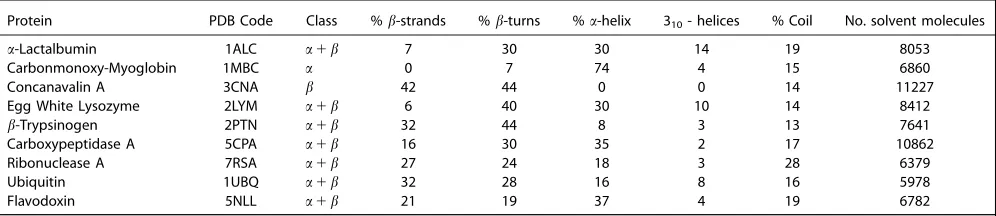
Table 2.Proteins studied with their PDB codes.

Protein PDB Code Class %b-strands %b-turns %a-helix 310- helices % Coil No. solvent molecules

a-Lactalbumin 1ALC a1b 7 30 30 14 19 8053

Carbonmonoxy-Myoglobin 1MBC a 0 7 74 4 15 6860

Concanavalin A 3CNA b 42 44 0 0 14 11227

Egg White Lysozyme 2LYM a1b 6 40 30 10 14 8412

b-Trypsinogen 2PTN a1b 32 44 8 3 13 7641

Carboxypeptidase A 5CPA a1b 16 30 35 2 17 10862

Ribonuclease A 7RSA a1b 27 24 18 3 28 6379

Ubiquitin 1UBQ a1b 32 28 16 8 16 5978

Flavodoxin 5NLL a1b 21 19 37 4 19 6782

16 cm21. The Hamiltonian is diagonalized and the corre-sponding unitary transformation is used to transform the tran-sition dipole matrix. The dipole approximation is used, whereby cross-excitations are not allowed. The 2D signal is evaluated as the sum of the rephasing and nonrephasing components. The computed spectra shown in this article are purely in the frequency domain, and the diagonal and off-diagonal contributions to the 2D signal shown here are posi-tive and negaposi-tive signals respecposi-tively (as in photon echo experiments). Thus the positive signal represents the ground state depletion (bleach) and stimulated emission (v50!1), while the negative signal corresponds to excited state emis-sion (v51!2). Polarization conditions have been examined previously by Hochstrasser.[82] The peak intensities are

collected by ensemble averaging the lab frame dipole moment components to account for the orientation of resi-dues with respect to the laser polarization. Our 2D signal is computed using theZZZZpolarization condition:

hZaZbZcZdi5 1

15 hcoshabcoshcdi1hcoshaccoshbdi1hcoshadcoshbci

(12)

wherehmnis the angle between transition dipolesmandn. In a later section, we show the enhancement of cross-peaks by subtracting two computed spectra: one using theZZZZ condi-tion and the other using the ZXXZ pulse condition.[63,80–83] Similar to eq. (12), the latter pulse condition can be expressed as:

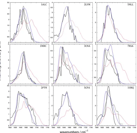
Figure 2. Amide I IR spectra of the nine proteins. The solid black line represents the experimental spectra from various sources cited by Torii and Tasumi, J. Chem. Phys., 1992, 96, 3379, reproduced by permission,[42]_{who reported that the spectra were “weakly deconvoluted”. The dashed black represents the}

experimental (recorded for 3% protein solution in H2O) transmission IR spectra taken from Karjalainen et al., J. Phys. Chem. B, 2012, 116, 4831, reproduced

by permission.[54]_{The dashed blue represents the average computed spectra including solvent, and the dotted red line represents the average computed}

hZaXbXcZdi52

1

30 hcoshabcos hcdi24hcoshaccoshbdi

1hcoshadcoshbciÞ (13)

The enhanced signal is computed using:

Sig_en5hZZZZi23hZXXZi (14)

Molecular dynamics simulations

Using the NAMD 2.9 molecular dynamics package,[84]we per-formed MD simulations on ubiquitin and the eight proteins studied by Torii and Tasumi.[42]The structures were taken from the Protein Data Bank, and the N- and C-termini were capped to give (NH1₃-CaH2) and (-CH2-CO22), respectively. For the cases of a-lactalbumin, concanavalin A and myoglobin, the apo

forms of the proteins were used. Neutralization was achieved by adding 9 Na1ions fora-lactalbumin, 9 K1for concanavalin A, 16 K1_{for flavodoxin, 2 Cl}-_{for myoglobin, 5 Cl}-_for ribonucle-ase A, 6 Cl-for trypsin, and 8 Cl-for lysozyme. The simulations included explicit water to model the influence of conforma-tional dynamics on line broadening, and to investigate the effect of solvation on the Amide I band. Each protein was sol-vated in a hexagonal prism of TIP3P water molecules,[85] and periodic boundary conditions were applied. To account for long-range interactions, the Particle Mesh Ewald method[86] was used, and the Lennard-Jones cutoff was 12 A˚ . Energy min-imization was performed for each protein for 30,000 cycles.

Thereafter an equilibration process with an integration time-step of 2 fs ran for 0.5 ns, during which all covalent bonds involving hydrogen were constrained using the SHAKE algo-rithm.[87] Experiments are usually performed in deuterated water. The water molecules in our simulations have rigid OAH bonds. Thus, the TIP3P model, captures hydrogen bonding and electrostatic effects but, neither the influence of the

vibrations of water nor the effect of the deuteration on the conformational dynamics of the protein are considered.

Production dynamics were performed for a period of 2 ns in the NPT ensemble using Langevin dynamics and a damping coefficient of 5 ps21. The Nose–Hoover[88–90]and Langevin pis-ton[91]periods were set to 100 fs and their time-decay period was set to 50 fs to keep the temperature constant at 300 K, while maintaining pressure at 1 atm. Snapshots were sampled uniformly every picosecond. Trajectory files with and without solvent were saved separately to investigate the effect of sol-vent on the computed spectra. The 2 ns trajectories are short, but the main purpose is to provide a sample of configurations close to the experimental structures. Our unconstrained simu-lations will potentially explore a broader and more physical range of equilibrium conformations than the constrained simu-lations of Choi et al.[63]

Results and Discussion

Experimental transmission IR spectra were taken from the litera-ture[42,63]rescaled such that the highest intensity peaks match the computed spectra, and plotted against the computed spec-tra of the nine proteins (Fig. 2). The experimental conditions used for recording the spectra cited by Torii and Tasumi[42]_were as follows:a-lactalbumin and lysozyme were recorded using a 3.5% protein solution in D2O; myoglobin and trypsin using a 5% protein solution in H2O, ribonuclease A using a 10% protein solution in H2O, while spectra for carboxypeptidase A, conca-navalin A, and flavadoxin spectra were all recorded using a 5% protein solution in D2O. We present our computed spectra with-out any post-processing to enhance the fine structure. The over-all band shape of each of the computed spectra for solvated proteins agrees with the experiment (Fig. 2).

The spectra computed neglecting the solvent exhibit an Amide I band that is broader than the experiment, extending beyond 1700 cm21 to around 1750 cm21. We believe that neglecting solvent in the calculations means that the surface

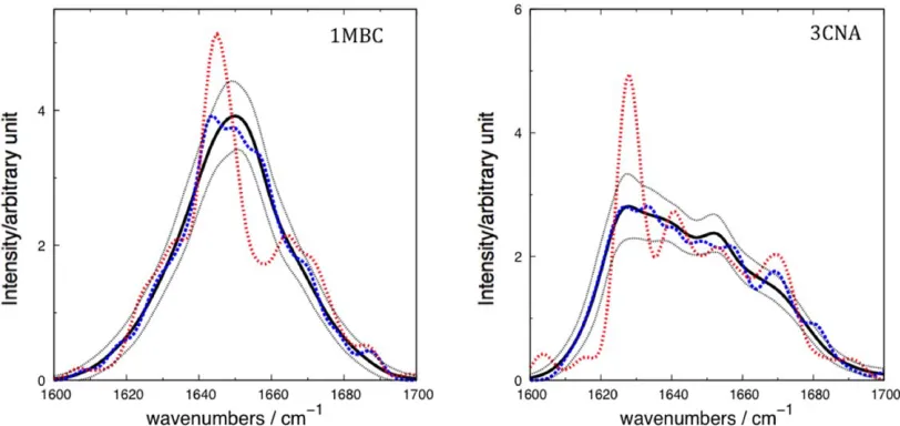
residues have an environment that is artefactually more differ-ent from the buried residues compared to the situation for a solvated system. To investigate the influence of conformational diversity on the computed spectra, we calculated the standard deviation of the computed intensity at each wavenumber over all snapshots (Fig. 3). We also identified the individual snap-shots giving rise to the computed spectra that were least and most similar to the mean computed spectra over the 2 ns sim-ulation period (Fig. 3).

The spectra from individual snapshots that are most dissimi-lar to the ensemble show some of the most intense features. By examining these conformations, we can characterize the extent of (de)localization of the vibrations associated with the most intense features. The squares of the eigenvector coeffi-cients reflect the contributions of the local modes to the tran-sition.[93,94]For the most dissimilar snapshot of concanavalin A, only two coefficients had a squared magnitude greater than 0.25, that is, none of the transitions was particularly localized. Of particular note was a pattern observed near the end of the 2 ns trajectory. The intense peak was located between 1622 and 1626 cm21. In this spectral region of the simulation, the vibration was delocalized across different residues in parallel strands. This is consistent with the strength of the through-space coupling constants between these residues. Figure 4 shows the location of the vibration in the context of the pro-tein structure. The coupling between the residues fluctuates over the simulation, but certain conformations (Fig. 4) exhib-ited strong inter-strand coupling between residues perpendic-ular to the strand orientation of the sheet, which is consistent with the findings of Woys et al.[95]

Experimentally,[96,97] it is possible using expressed protein ligation and native chemical ligation to isotope label distinct regions in proteins, for example, specific elements of secondary structure. The computational analogue is readily performed and

can help us to understand the various contributions to the spec-tra and deconvolute the overlapping bands of the 1D signal. We illustrate this for the simulations of solvated ubiquitin. The result of isotope labeling of either residues ina-helices or inb-sheets (Fig. 5) shows a shift in peaks accordingly. The residues belong-ing toa-helices show a contribution to the 1D signal in the form of a single broad peak at 1580 cm21, while the contribution fromb-sheet residues shows two peaks, one more intense than the other. Splitting the signal by isotope labeling has an effect on the overall band maxima, which will be discussed later.

Karjalainen et al.[54]assumed the shift in intrinsic frequency is related to the presence or absence of a hydrogen bond between a carbonyl oxygen of one amide group and an amide hydrogen of another. We investigated the relationship between shift in intrinsic frequency and the presence of hydrogen bonds to solvent. The relationship is evident, but appears to be a weak one (Fig. 6). For example, in the case of thea-helical carbonmonoxy-myoglobin, the number of hydro-gen bonds to solvent molecules shows a modest influence on the extent of the negative shift from the central frequency, as is expected. Concanavalin A, ab-sheet protein, shows a weaker but similar trend. Our modeling of the influence of hydrogen bonds is through the electrostatic potential, which is a non-local approach. It may be that a more explicit treatment of hydrogen bonding would identify a stronger relationship between hydrogen bonding and the frequency shift.

2D IR spectra

Conformational dynamics of the protein and solvent are reflected in the 2D lineshapes. We have computed the absorp-tive 2D IR spectra for ubiquitin, concanavalin A, carbonmonoxy-myoglobin, lysozyme, ribonuclease A, anda-lactalbumin based on the conformations sampled from the MD trajectories. We

chose these proteins as a benchmark due to their different sizes and mixed structural compositions. For ubiquitin, we investigated the convergence of the computed spectra with the number of conformations sampled from the MD trajectory. Spectra computed with 200 snapshots sampled uniformly across the trajectory gave a computed spectrum very similar to that computed with 2000. So the 2D-spectra for the larger pro-teins were computed with 200 snapshots to limit the computa-tional cost. Thus inhomogeneous broadening in the calculated 2D spectra is a result of the structural changes depicted by the snapshots, and homogeneous broadening was modeled by convoluting with a 2D Lorentzian bandwidth of 10 cm21. The vibrational motional narrowing effect, whereby the line width may be overestimated by static structural snapshots,[98–100] may influence the computed spectrum. Whilst this is a signifi-cant effect for NMA in solution,[49] it may be less important for polypeptides, because of the spread of the multiple amide modes of the protein.[101] Different features can be seen in the spectra (Fig. 7). The intense peaks which are plotted with pump frequency,x1, on the horizontal axis and the probe fre-quency, x3, on the vertical axis as in Ref. 102 correspond to contributions from thea-helices [x1,x3]5[1635, 1635] cm

21

in the case of ubiquitin. For concanavalin A, the anti-parallel sheet contribution can be seen as a weak peak appearing at [1660, 1660] cm21. Two intense signals are also seen between [1625, 1625] cm21_{, both associated with out-of-phase} oscilla-tions of carbonyls of the same b-strand.[74] A broad peak stretches along the diagonal from [1620, 1620] cm21 to [1670, 1670] cm21_{. This agrees with experiment}[102] _{and is} associated with random coils in concanavalin A. Random coils probably contribute to the weaker signal at [1660, 1660] cm21_.

In all spectra shown in Figure 7, the elongation along the diagonal stretches from 1620 to 1670 cm21 and shows that the solvent-exposed residues experience a fluctuating

electrostatic environment, due to conformational disorder and fluctuations of the solvent. The spectrum of carbonmonoxy-myoglobin is dominated by contributions from a-helices. A broad and intense signal stretches from [1640, 1640] to [1655, 1655] cm21_{. This is also seen fora-lactalbumin [1630, 1630] to} [1660, 1660] cm21. Table 3 summarizes the location of the peak centers in the computed and the experimental spectra of Figure 7. Overall, our computed spectra agree well with the experimental spectra. The level of agreement is comparable with recently reported calculations[64,65] using different force fields and modeling protocols.

More detailed information can be accessed by enhancing the cross-peaks (Fig. 8). For example, coupled vibrations of dif-ferent transitions are now revealed compared to the ZZZZ

spectra. The cross-polarization hZZZZi23hZXXZi signal sup-presses the diagonals to some extent and enhances other fea-tures of the 2D spectra. The off-diagonal peaks are better resolved than their counterparts in Figure 7, allowing the nature of the coupling between different local modes to be explored further. Much weaker peaks appear on the diagonal in Figure 8 compared to the intense diagonal peaks in Figure 7. These weak diagonal peaks (Fig. 8) are now comparable in intensity with the off-diagonal cross-peaks, and these features merge somewhat to give a broad peak which extends parallel to thex1axis, as can be seen for example in the case of con-canavalin A: peak I, Figure 8. The splitting between the posi-tive and the negaposi-tive signals of a cross-peak is a measurement of the coupling strength and is due to the off-diagonal anhar-monicity. For example in concanavalin A, peak I indicates there is a strong coupling between structural elements, while in the rest of the proteins the analogous peak indicates weaker cou-pling. Table 4 summarizes the cross-peaks highlighted in Fig-ure 8.

In the cross-polarization spectra of a-lactalbumin and myo-globin (Fig. 8), there are signs of contribution from coupled

Figure 5. Computed 1D spectra of ubiquitin (1UBQ) with13_C18_{O isotope labeling of thea-helix residues a), andb-sheet residues b). The solid black line in}

unstructured coils. Unstructured coils appear as broad feature-less peaks at [x1, x3]51650 or 1660 cm21,[79] and the cross-polarization spectra reveal broad peaks stretching from 1660 cm21

toward 1680 cm21

due to b-strands coupled with unstructured coils (in the case of a-lactalbumin: peak IV), and coupled unstructured coils with b -turns (in the case of myo-globin: peak III). The shape of the two cross peaks is different and the finding agrees with a previous study[103] to suppress random coil features.

Cross-peaks usually come in pairs, but when one half of the doublet is more intense (as is the case in peak IV for lactalbumin and myoglobin), it generally means that the off-diagonal anharmonicity is weak between the two local sites.[80]The splitting between the diagonal and off-diagonal peaks is underestimated in Figure 7, which may suggest that

the value of the anharmonicity used in the calculations should be greater. Choi et al.[63]and Chung et al.[104] previ-ously investigated ubiquitin in two separate studies. Their spectra exhibited a Z-shape, due to the contribution from anti-parallel b-sheet strands. We find a similar Z-shape in both our ubiquitin and concanavalin A crossed-polarization spectra (Fig. 8).

The crossed-polarization spectroscopy is clearly a powerful, experimentally realizable approach, which provides an addi-tional insight into the origins of the 2D signal. Some of these origins can also be explored using different computational strategies. We investigate the contributions to the 2D signal by isotope labeling thea-helices andb-strand secondary struc-tures of ubiquitin. Figure 9 shows the two cases when either the helices or the sheets are labeled.

Both isotope labeled components have been shifted to 1570 cm21

and are consistent with the computed 1D spectra (Fig. 5). The diagonal peak intensities for the labeleda-helices are clearly much weaker than those for the rest of the protein. This is more evident in the 2D spectra as the signal is

proportional to the fourth power of the transition dipole moment, whereas in the 1D spectra, the intensity depends on the square of the transition dipole moment. The cross-peak at [1660, 1560] cm21in Figure 9b indicates coupling between b-sheet and random coil components. The absence of an anal-ogous cross-peak in Figure 9a indicates there is little or no cou-pling between b-sheet and a-helices. We have computed the 2D spectra of thea-helices andb-sheets separately (Fig. 10).

There are 12 residues in a-helices and 26 residues in b -strands. Two Hamiltonians were constructed in which the size of the one-quantum Hamiltonian was 12312 in the first case and 26 3 26 in the second, with all elements in the environ-ment: main chain, side chains, and solvent molecules contrib-uting to the electrostatic potential and shift in frequency. Figure 10 shows the contributions to the signal from both a -helices and b-strands. The b-sheet spectrum is about four times more intense than the a-helices spectrum consistent with the 2:1 ratio observed for the 1D spectrum. The contribu-tion from the a-helices is a diagonal elongated peak with its center at [1640, 1640] cm21 _{while the b-strands contribute} three peaks: two intense ones at [1625,1625] and [1638, 1638] cm21 and a weak one at[1660, 1660] cm21

indicating coupled local modes. There is also a weak cross-peak at [1680,

Figure 7. Experimental[102]_{and computed 2D absorptive spectra using theZZZZscheme for:a-lactalbumin (1ALC), carbonmonoxy-myoglobin (1MBC),}

ubiq-uitin (1UBQ), concanavalin A (3CNA), lysozyme (2LYM), and ribonuclease A (7RSA). Time delay (t2) in both the experimental and computed spectra was

zero. The contours for the computed spectra are plotted with a 10% intensity of the maximum amplitude with 20 uniformly spread contours from the min-imum to the maxmin-imum intensity. [Color figure can be viewed at wileyonlinelibrary.com]

Table 3.Locations of diagonal and off-diagonal peaks in the computed and experimental[102]_{2D-IR spectra.}

Diagonal peak locations (x15x3)/cm21

Protein Experiment Computed

1ALC 1645 1650

1MBC 1650 1647

1UBQ 1640 1635

2LYM 1640 1635

7RSA 1640 1640

3CNA 1620 1625

Off-diagonal peak locations (x1,x3)/cm21

Protein Experiment Computed

1ALC (1640,1610) (1640,1630)

1MBC (1640,1610) (1640,1635)

1UBQ (1640,1610) (1630,1625)

2LYM (1640,1620) (1630,1620)

7RSA (1640,1620) (1620,1620)

1620] cm21(Peak I). The presence of Peak I in Figures 10b and Peaks I and II Figure 9a is further indication of the coupling betweenb-secondary structure components.

Transition dipole strengths

Non-linear spectroscopies are more sensitive to transition dipole strengths than linear spectroscopies. The 2D intensities

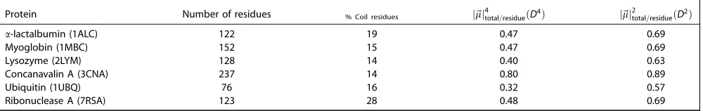
scale as j~lj4 compared to 1D intensities that scale as j~lj2. Grechko and Zanni[66]studied the 1D and 2D IR of a modela -helical system and concluded that the transition dipole strength of the random coil state is 0.12 D2, and that a greater magnitude indicates a more ordered system with vibrational excitonic states forming associated with secondary structure. Here, we extend that consideration to six of the proteins, extracting the two-quantum transition dipole moments that contribute to the 2D diagonal signal. In Table 5, we compare the per residue contribution to the 2D intensities,j~lj4total

residue for the aforementioned proteins. The absolute value of the transi-tion dipole,j~lj4_total was computed as a sum over all transition dipole moments. One might anticipate that more ordered structures such as concanavalin A should give more delocal-ized excitons, which should be manifested in more intense bands.

The per residue contribution, j~lj2total

residue which is computed here by taking the square root of j~lj4total

residue, confirms delocal-ized excitonic vibrations as expected from ordered

Figure 8. Computed<ZZZZ>23<ZXXZ>cross-peak 2D IR absorptive spectra computed fora-lactalbumin (1ALC), myoglobin (1MBC), ubiquitin (1UBQ), and concanavalin A (3CNA). Cross-peaks are highlighted with white dotted squares. The contours are plotted with a 10% intensity of the maximum ampli-tude with 20 uniformly spread contours from the minimum to the maximum intensity. [Color figure can be viewed at wileyonlinelibrary.com]

Table 4.The cross-peaks in the cross-polarization 2D-IR spectra (Fig. 8) fora-lactalbumin (1ALC), carbonmonoxy-myoglobin (1MBC), ubiquitin (1UBQ) and concanavalin A (3CNA).

Protein Peak (strength)

Structural components involved

1ALC I (w) II (w) III (w) IV (w) b a1b b b1coil

1MBC I (w) II (w) III (w) a a a1coil

1UBQ I (w) II (w) a b

3CNA I (s) II (w) b b

structured systems, and all the values fall above the thresh-old observed by Grechko and Zanni.[66] _{However, there is} not an obvious relationship between the proportion of coil structure in the protein and the intensity of the 2D diagonal

signal. This discrepancy might be explained by the fact coil structures in folded proteins do not necessarily have the same properties as random coils in unfolded peptides such as the ones studied by Grechko and Zanni.[66]

Figure 9. Computed 2D absorptive spectra using theZZZZ scheme of cases where thea- helices a) andb-strands b) of ubiquitin (1UBQ) are isotope labeled. The contours are plotted with a 10% intensity of the maximum amplitude and 20 uniformly spread contours from the minimum to the maximum intensity for the left panel and 20 similar uniformly spread contours for the right panel. The isotope labeled components are highlighted with red dotted squares and the cross peaks with white dotted ones. [Color figure can be viewed at wileyonlinelibrary.com]

Figure 10. Computed 2D absorptive spectra using theZZZZscheme ofaa) andbb) secondary structure separately of ubiquitin (1UBQ). The contours are plotted with a 10% intensity of the maximum amplitude and 20 uniformly spread contours from the minimum to the maximum intensity for the left panel and 20 similar uniformly spread contours for the right panel. Cross-peaks are highlighted with white dotted squares. [Color figure can be viewed at wileyonlinelibrary.com]

Table 5.The studied proteins (with PDB codes), the number of residues, and fraction of coil composition, the two-quantum transition dipole strengths per residuej~lj4

total residue.

Protein Number of residues % Coil residues j~lj

4

total=residueD 4

ð Þ j~lj2total=residueD 2 ð Þ

a-lactalbumin (1ALC) 122 19 0.47 0.69

Myoglobin (1MBC) 152 15 0.47 0.69

Lysozyme (2LYM) 128 14 0.40 0.63

Concanavalin A (3CNA) 237 14 0.80 0.89

Ubiquitin (1UBQ) 76 16 0.32 0.57

Ribonuclease A (7RSA) 123 28 0.48 0.69

Conclusion

Overall, the calculations have quantitatively reproduced 1D-IR spectra for the proteins studied. We have investigated the sensi-tivity of the Amide I peaks to conformational dynamics. Our motivation was to investigate the effect of conformational dynamics on the overall lineshapes. The mixing of the local modes that underlies the 1D-IR spectra is revealed more explic-itly, although not with complete clarity in the 2D-IR spectra. Our study shows that the Cho model[47] in combination with MD simulations confirm the importance of conformational dynamics in affecting the overall absorbance. We would expect different maps[50,55–60]would yield qualitatively similar findings, although some of the quantitative detail might vary.[62,105]

The computed 2DIR spectra for ubiquitin, carbonmonoxy-myoglobin,a-lactalbumin, concanavalin A, flavadoxin, and ribonu-clease A are broadly in agreement with that presented in previous studies.[62,63,102,104]Solvation plays a significant role in the nature of the computed spectra. Through calculations of the Amide I band and analysis of the exciton Hamiltonian matrix, it is possible to relate specific conformational features to the IR spectrum. Delv-ing deeper into the dynamics of proteins and studyDelv-ing sDelv-ingle snapshots for both concanvalin A and carbonmonoxy-myoglobin provides a stepping stone to understanding the appearance of the 2D spectra. The width of the 1D spectra is reflected in the linewidth of the diagonal on the 2D spectra. The off-diagonal cross peaks were enhanced for ubiquitin, carbonmonoxy-myoglobin,a-lactalbumin, and concanavalin A by computing the hZZZZi23hZXXZi spectra for each case. We explored whether there is a relationship between the contribution to the 2D diago-nal sigdiago-nal and the fraction of random coil, but none was evident. We are currently studying the dynamics and 2D IR spectroscopy of protein-ligand binding, and investigating the behavior of cou-pled modes during binding and dissociation.

Acknowledgments

We thank Rachel Hill and Nick Besley (University of Nottingham) for helpful discussions. We are grateful for access to the University of Nottingham High Performance Computing facility and to the Mid-Plus Regional Centre of Excellence for Computational Science, Engi-neering and Mathematics; this work was supported by the Engineering and Physical Sciences Research Council [grant number EP/K000128/1].

Keywords: two-dimensional infrared spectroscopy

How to cite this article: F. S. Husseini, D. Robinson, N. T. Hunt, A. W. Parker, J. D. Hirst. J. Comput. Chem. 2016, DOI: 10.1002/jcc.24674

[1] A. Elliott, E. J. Ambrose,Nature1950,165, 921. [2] S. Krimm,Biopolymers1983,22, 217.

[3] S. Krimm, J. Bandekar,Adv. Prot. Chem.1986,38, 181. [4] F. Siebert,Method Enzymol.1995,246, 501.

[5] J. M. Chalmers, P. R. Griffiths, Handbook of Vibrational Spectroscopy; Wiley-Blackwell, New Jersey, USA,2002.

[6] A. K. Dioumaev,Biochemistry (Moscow)2001,66, 1269. [7] H. Susi, D. M. Byler,Method Enzymol.1986,130, 290. [8] A. Dong, P. Huang, W. S. Caughey,Biochemistry1990,29, 3303. [9] W. K. Surewicz, H. H. Mantsch,Biochim. Biophys. Acta1988,952, 115. [10] H. Susi, D. M. Byler,Biochem. Biophys. Res. Commun.1983,115, 391. [11] S. Y. Venyaminov, N. N. Kalnin,Biopolymers1990,30, 1243.

[12] N. N. Kalnin, I. A. Baikalov, S. Y. Venyaminov,Biopolymers 1990, 30, 1273.

[13] H. Torii, M. Tasumi,J. Raman Spectrosc.1998,29, 81. [14] C. Lee, M. H. Cho,J. Phys. Chem. B2004,108, 20397. [15] Y. Tanimura, S. Mukamel,J. Chem. Phys.1993,99, 9496.

[16] P. Hamm, M. H. Lim, R. M. Hochstrasser,J. Phys. Chem. B1998,102, 6123.

[17] M. C. Asplund, M. T. Zanni, R. M. Hochstrasser, Proc. Natl. Acad. Sci. USA2000,97, 8219.

[18] M. T. Zanni, S. Gnanakaran, J. Stenger, R. M. Hochstrasser, J. Phys. Chem. B2001,105, 6520.

[19] O. Golonzka, M. Khalil, N. Demirdoven, A. Tokmakoff,Phys. Rev. Lett.

2001,86, 2154.

[20] P. Hamm, R. M. Hochstrasser, M. D. Fayer, Ultrafast Infrared and Raman Spectroscopy; Dekker, New York,2001.

[21] S. Woutersen, P. Hamm,J. Chem. Phys.2001,114, 2727.

[22] N. H. Ge, M. T. Zanni, R. M. Hochstrasser,J. Phys. Chem. A2002,106, 962.

[23] I. V. Rubtsov, J. P. Wang, R. M. Hochstrasser,Proc. Natl. Acad. Sci. USA

2003,100, 5601.

[24] J. Park, R. M. Hochstrasser,J. Chem. Phys.2006,323, 78.

[25] Y. S. Kim, J. P. Wang, R. M. Hochstrasser,J. Phys. Chem. B2005,109, 7511.

[26] C. Fang, J. Wang, Y. S. Kim, A. K. Charnley, W. Barber-Armstrong, A. B. Smith, S. M. Decatur, R. M. Hochstrasser,J. Phys. Chem. B 2004,108, 10415.

[27] H. Ishikawa, K. Kwak, J. K. Chung, S. Kim, M. D. Fayer,Proc. Natl. Acad. Sci. USA2008,105, 8619.

[28] H. Ishikawa, I. J. Finkelstein, S. Kim, K. Kwak, J. K. Chung, K. Wakasugi, A. M. Massari, M. D. Fayer,Proc. Natl. Acad. Sci. USA2007,104, 16116. [29] K. Adamczyk, N. Simpson, G. M. Greetham, A. Gumiero, M. A. Walsh,

M. Towrie, A. W. Parker, N. T. Hunt,Chem. Sci.2015,6, 505.

[30] D. Zimdars, A. Tokmakoff, S. Chen, S. R. Greenfield, M. D. Fayer, T. I. Smith, H. A. Schwettman,Phys. Rev. Lett.1993,70, 2718.

[31] Y. S. Kim, L. Liu, P. H. Axelsen, R. M. Hochstrasser,Proc. Natl. Acad. Sci. USA2009,106, 17751.

[32] C. T. Middleton, P. Marek, P. Cao, C. C. Chiu, S. Singh, A. M. Woys, J. J. Pablo, D. P. Raleigh, M. T. Zanni,Nat. Chem.2012,4, 355.

[33] D. B. Strasfeld, Y. L. Ling, S. H. Shim, M. T. Zanni,J. Am. Chem. Soc.

2008,130, 6698.

[34] S. H. Shim, D. B. Strasfeld, Y. L. Ling, M. T. Zanni,Proc. Natl. Acad. Sci. USA2007,104, 14197.

[35] A. Remorino, I. V. Korendovych, Y. B. Wu, W. F. DeGrado, R. M. Hochstrasser,Science2011,332, 1206.

[36] A. Ghosh, J. Qiu, W. F. DeGrado, R. M. Hochstrasser,Proc. Natl. Acad. Sci. USA2011,108, 6115.

[37] J. Manor, P. Mukherjee, Y. S. Lin, H. Leonov, J. L. Skinner, M. T. Zanni, I. T. Arkin,Structure2009,17, 247.

[38] Z. Ganim, H. S. Chung, A. W. Smith, L. P. Deflores, K. C. Jones, A. Tokmakoff,Acct. Chem. Res.2008,41, 432.

[39] R. M. Hochstrasser,Proc. Natl. Acad. Sci. USA2007,104, 14190. [40] K. Adamczyk, M. Candelaresi, K. Robb, A. Gumiero, M. A. Walsh, A. W.

Parker, P. A. Hoskisson, N. P. Tucker, N. T. Hunt, Meas. Sci. Technol.

2012,23, 062001.

[41] N. T. Hunt,Chem. Soc. Rev.2009,38, 1837. [42] H. Torii, M. Tasumi,J. Chem. Phys.1992,96, 3379. [43] P. Hamm, S. Woutersen,Bull. Chem. Soc. Jpn.2002,75, 985.

[44] J. W. Brauner, C. R. Flach, R. Mendelsohn,J. Am. Chem. Soc.2005,127, 100.

[45] S. Y. Cha, S. H. Ham, M. H. Cho,J. Chem. Phys.2002,117, 740. [46] J. H. Choi, S. Ham, M. Cho,J. Chem. Phys.2002,117, 6821. [47] S. Ham, M. Cho,J. Chem. Phys.2003,118, 6915.

[49] K. Kwac, M. Cho,J. Chem. Phys.2003,119, 2247.

[50] T. M. Watson, J. D. Hirst,Phys. Chem. Chem. Phys.2004,6, 998. [51] T. M. Watson, J. D. Hirst,Mol. Phys.2005,103, 1531.

[52] P. Bour, T. A. Keiderling,J. Chem. Phys.2003,119, 11253. [53] P. Bour, T. A. Keiderling,J. Phys. Chem. B2005,109, 5348.

[54] E. L. Karjalainen, T. Ersmark, A. Barth,J. Phys. Chem. B2012,116, 4831. [55] T. Hayashi, W. Zhuang, S. Mukamel,J. Phys. Chem. A2005,109, 9747. [56] T. L. Jansen, J. Knoester,J. Chem. Phys.2006,124, 044502.

[57] T. L. Jansen, A. G. Dijkstra, T. M. Watson, J. D. Hirst, J. Knoester, J. Chem. Phys.2006,125, 44312.

[58] H. Torii, T. Tatsumi, T. Kanazawa, M. Tasumi, J. Phys. Chem. B1998,

102, 309.

[59] J. R. Schmidt, S. A. Corcelli, J. L. Skinner, J. Chem. Phys. 2004, 121, 8887.

[60] Y. S. Lin, J. M. Shorb, P. Mukherjee, M. T. Zanni, J. L. Skinner,J. Phys. Chem. B2009,113, 592.

[61] N. G. Mirkin, S. Krimm,J. Am. Chem. Soc.1991,113, 9742. [62] Z. Ganim, A. Tokmakoff,Biophys. J.2006,91, 2636.

[63] J. H. Choi, H. Lee, K. K. Lee, S. Hahn, M. Cho,J. Chem. Phys.2007,126, 045102.

[64] A. S. Bondarenko, T. L. C. Jansen,J. Chem. Phys.2015,142, 212437. [65] A. V. Cunha, A. S. Bondarenko, T. L. C. Jansen,J. Chem. Theory Comput.

2016,12, 3982.

[66] M. Grechko, M. T. Zanni,J. Chem. Phys.2012,137, 184202.

[67] A. S. Davydov, The Theory of Molecular Excitons; McGraw-Hill, New York,1962.

[68] B. M. Bulheller, J. D. Hirst,Bioinformatics2009,25, 539.

[69] R. B. Best, X. Zhu, J. Shim, P. E. M. Lopes, J. Mittal, M. Feig, A. D. MacKerell,J. Chem. Theor. Comput.2012,8, 3257.

[70] A. D. MacKerell, M. Feig, C. L. Brooks,J. Comput. Chem.2004,25, 1400. [71] A. D. MacKerell, D. Bashford, M. Bellott, R. L. Dunbrack, J. D. Evanseck, M. J. Field, S. Fischer, J. Gao, H. Guo, S. Ha, D. Joseph-McCarthy, L. Kuchnir, K. Kuczera, F. T. Lau, C. Mattos, S. Michnick, T. Ngo, D. T. Nguyen, B. Prodhom, W. E. Reiher, B. Roux, M. Schlenkrich, J. C. Smith, R. Stote, J. Straub, M. Watanabe, J. Wiorkiewicz-Kuczera, D. Yin, M.

Karplus,J. Phys. Chem. B1998,102, 3586.

[72] J. Huang, A. D. MacKerell,J. Comput. Chem.2013,34, 2135.

[73] D. Abramavicius, W. Zhuang, S. Mukamel,J. Phys. Chem. B2004,108, 18034.

[74] M. Reppert, A. Tokmakoff,J. Chem. Phys.2013,138, 134116.

[75] S. Roy, J. Lessing, G. Meisl, Z. Ganim, A. Tokmakoff, J. Knoester, T. L. C. Jansen,J. Chem. Phys.2011,135, 234507.

[76] C. Fang, J. Wang, A. K. Charnley, W. Barber-Armstrong, A. B. Smith, S. M. Decatur, R. M. Hochstrasser,Chem. Phys. Lett.2003,382, 586. [77] L. Wang, C. T. Middleton, M. T. Zanni, J. L. Skinner,J. Phys. Chem. B

2011,115, 3713.

[78] L. Wang, C. T. Middleton, S. Singh, A. S. Reddy, A. M. Woys, D. B. Strasfeld, P. Marek, D. P. Raleigh, J. J. Pablo, M. T. Zanni, J. L. Skinner,J. Am. Chem. Soc.2011,133, 16062.

[79] M. D. Fayer, Ultrafast Infrared Vibrational Spectroscopy; CRC Press, Boca Raton,2013.

[80] M. T. Zanni, P. Hamm, Concepts and Methods of 2D Infrared Spectros-copy; Cambridge University Press, Cambridge,2013.

[81] M. Khalil, N. Demirdoven, A. Tokmakoff,€ J. Phys. Chem. A2003, 107, 5258.

[82] R. M. Hochstrasser,Chem. Phys.2001,266, 273.

[83] J. Dreyer, A. M. Moran, S. Mukamel,Bull. Korean Chem. Soc.2003,24, 1091.

[84] J. C. Phillips, R. Braun, W. Wang, J. Gumbart, E. Tajkhorshid, E. Villa, C. Chipot, R. D. Skeel, L. Kale, K. Schulten,J. Comput. Chem.2005,26, 1781. [85] W. L. Jorgensen, J. Chandrasekhar, J. D. Madura, R. W. Impey, M. L.

Klein,J. Chem. Phys.1983,79, 926.

[86] T. Darden, D. York, L. Pedersen,J. Chem. Phys.1993,98, 10089. [87] J. P. Ryckaert, G. Ciccotti, H. J. C. Berendsen,J. Comput. Phys.1977,23,

327.

[88] G. J. Martyna, D. J. Tobias, M. L. Klein,J. Chem. Phys.1994,101, 4177. [89] S. Nose,J. Chem. Phys.1984,81, 511.

[90] W. G. Hoover,Phys. Rev. A1985,31, 1695.

[91] S. E. Feller, Y. H. Zhang, R. W. Pastor, B. R. Brooks,J. Chem. Phys.1995,

103, 4613.

[92] E. G. Hutchinson, J. M. Thornton,Prot. Sci.1996,5, 212. [93] H. Torii,J. Phys. Chem. A2004,108, 2103.

[94] M. Lima, R. Chelli, V. V. Volkov, R. Righini,J. Chem. Phys. 2009, 130, 204518.

[95] A. M. Woys, A. M. Almeida, L. Wang, C. C. Chiu, M. McGovern, J. J. Pablo, J. L. Skinner, S. H. Gellman, M. T. Zanni,J. Am. Chem. Soc.2012,

134, 19118.

[96] S. D. Moran, S. M. Decatur, M. T. Zanni,J. Am. Chem. Soc.2012,134, 18410.

[97] L. E. Buchanan, J. K. Carr, A. M. Fluitt, A. J. Hoganson, S. D. Moran, J. J. Pablo, J. L. Skinner, M. T. Zanni, Proc. Natl. Acad. Sci. USA2014,111, 5796.

[98] J. D. Eaves, A. Tokmakoff, P. L. Geissler,J. Phys. Chem. A2005, 109, 9424.

[99] J. D. Smith, R. J. Saykally, P. L. Geissler,J. Am. Chem. Soc.2007,129, 13847.

[100] B. M. Auer, J. L. Skinner,J. Chem. Phys.2007,127, 104105. [101] W. R. W. Welch, J. Kubelka,J. Phys. Chem. B2012,116, 10739.2. [102] C. R. Baiz, C. S. Peng, M. E. Reppert, K. C. Jones, A. Tokmakoff,Analyst

2012,137, 1793.

[103] C. T. Middleton, L. E. Buchanan, E. B. Dunkelberger, M. T. Zanni,J. Phys. Chem. Lett.2011,2, 2357.

[104] H. S. Chung, M. Khalil, A. W. Smith, Z. Ganim, A. Tokmakoff, Proc. Natl. Acad. Sci. USA2004,102, 612.

[105] A. M. Woys, Y. S. Lin, A. S. Reddy, W. Xiong, J. J. Pablo, J. L. Skinner, M. T. Zanni,J. Am. Chem. Soc.2010,132, 2832.