Efficient calculation of molecular integrals over
London atomic orbitals
Tom J. P. Irons, Jan Zemen, and Andrew M. Teale
∗School of Chemistry, University of Nottingham, University Park, Nottingham NG7 2RD, United Kingdom
E-mail: [email protected]
Abstract
The use of London atomic orbitals (LAOs) in a non-perturbative manner enables the deter-mination of gauge-origin invariant energies and properties for molecular species in arbitrarily strong magnetic fields. Central to the effi-cient implementation of such calculations for molecular systems is the evaluation of molec-ular integrals, particmolec-ularly the electron repul-sion integrals (ERIs). We present an imple-mentation of several different algorithms for the evaluation of ERIs over Gaussian-type LAOs at arbitrary magnetic field strengths. The efficiency of generalized McMurchie-Davidson (MD), Head-Gordon-Pople (HGP) and Rys quadrature schemes is compared. For the Rys quadrature implementation, we avoid the use of high precision arithmetic and interpolation schemes in the computation of the quadrature roots and weights, enabling the application of this algorithm seamlessly to a wide range of magnetic fields. The efficiency of each gen-eralised algorithm is compared by numerical application, classifying the ERIs according to their total angular momenta and evaluating their performance for primitive and contracted basis sets. In common with zero-field integral evaluation, no single algorithm is optimal for all angular momenta thus a simple mixed scheme is put forward, which selects the most efficient approach to calculate the ERIs for each shell quartet. The mixed approach is significantly more efficient than the exclusive use of any
in-dividual algorithm.
1
Introduction
In recent years, there has been a great deal of interest in the non–perturbative calcula-tion of molecular energies and properties in the presence of arbitrarily strong magnetic fields.1–12 Investigations have included the
im-plementation of electronic structure calcula-tions at the Hartree-Fock,1,8 configuration–
interaction,4 coupled-cluster,9 coupled-cluster
equation of motion12 and current
density-functional6,10,11 levels of theory. Underpinning
the implementations of these methods has been the use of Gaussian type London atomic or-bitals13,14 (LAOs). LAOs consist of standard
Gaussian basis functions multiplied by a field-dependent plane-wave phase factor, allowing results independent of gauge-origin to be ob-tained using finite basis sets.
One of the principle challenges in these cal-culations is the the evaluation of molecular integrals over LAOs. A number of algorithms have been put forward for the evaluation of electron repulsion integrals (ERIs) over LAOs including generalized Obara–Saika,15–17
accom-panying coordinate expansion,18,19Rys
quadra-ture,8,20,21 and McMurchie–Davidson1,22–24
schemes. In particular, the McMurchie– Davidson scheme has been employed in the
London quantum chemistry program25 and a
version of the Rys quadrature scheme in the
A number of advantageous features for in-tegral schemes to perform non-perturbative calculations with arbitrary strength magnetic fields can be identified. The first of these is that the algorithmic complexity should not be signif-icantly increased over the corresponding zero-field scheme. The second is that they should be applicable to arbitrarily high angular momenta functions, in order to allow sufficient flexibil-ity for the description of anisotropic changes in the electronic structure upon application of a magnetic field. The third feature is that they should be efficient for application to both con-tracted and primitive functions, since the lat-ter may provide additional basis set flexibility in high field applications.
In common with integral schemes at zero field, no single algorithm can satisfy all of these re-quirements simultaneously. Indeed, each al-gorithm inherently has its own strengths and weaknesses; often the most effective approach is to use several algorithms and select the most efficient for each integral class extemporane-ously. In this work we explore generalized al-gorithms based on the McMurchie–Davidson (MD), Head-Gordon Pople (HGP) and Rys quadrature methods.
It has been shown that the generalzed MD al-gorithm is significantly more complex than the standard equivalent, requiring many more in-termediates, thus does not exhibit the same effi-ciency or scaling. In contrast, the HGP method can be generalized without increasing the un-derlying complexity of the algorithm; here we present an implementation of this approach for the first time. A generalized Rys quadrature has been explored previously, however its use was limited to low field strengths owing to the fact that the required quadrature roots and weights were being approximated by a 2D in-terpolation scheme. Whilst adequate for this purpose, the application of this approach to ar-bitrary field strengths is problematic as it would necessitate the storage of very large interpola-tion grids. In addiinterpola-tion, it was noted in Ref. 8 that high-precision arithmetic was necessary to determine the required parameters. In this work, we generalize the Rys quadrature ap-proach to a much wider range of field strengths
using the approach put forward by Flocke27 to
compute the roots and weights when required. We commence in Section 2 by discussing some preliminaries, including the use of shell-pair quantities and the transformation between Cartesian and spherical harmonic Gaussians. In Section 3, we discuss the calculation of the one-electron integrals required for practical cal-culations, including the generalization of the ki-netic energy integrals associated with the in-troduction of a vector potential describing the magnetic field. In Section 4 we describe three approaches to the calculation LAO-ERIs, com-paring their relative algorithmic complexity. In Section 5, relative timings for each approach are discussed, illustrating the relative advan-tages and disadvanadvan-tages of each algorithm. A mixed scheme, which selects the most efficient algorithm for each class of integral extempora-neously is presented. This mixed approach pro-vides an an effective approach to minimizing the computational cost of the LAO-ERI evaluation.
2
Preliminaries and shell–
pair data
In this work we are concerned with the evalua-tion of molecular integrals over Gaussian–type LAOs. A standard unnormalized Gaussian– type orbital (GTO) has the general form
φa(r) = (x−Ax)ax(y−Ay)ay(z−Az)az Ka
X
k=1
dke−αk|r−A|
2
(1)
where the function is centred at A = (Ax,Ay,Az), has angular momentum a =
(ax, ay, az) and has exponents {αk} with
re-spective contraction coefficient {dk}. Where
the contraction length Ka is equal to 1, the
GTO only has one exponent with a corre-sponding contraction coefficient of 1.0 and is a primitive GTO, whereas if Ka >1 the GTO
is contracted. Gaussian–type LAOs are similar to standard GTOs, differing by a phase factor
ωa(r) = φa(r)e−ika·r (2)
wherekais the wave vector of the London plane
external magnetic field B and relative to the gauge–originO.
In contemporary molecular integral codes, in-tegrals are almost always computed in shell– batches rather than individually;28 a shell
com-prises all basis functions with common cen-tre, exponent and total angular momentum
La = ax+ay +az but with different
distribu-tions between the three Cartesian components. It is highly advantageous to compute integrals in shell–batches as integrals between individual GTOs within the shells have many common in-termediates which may be re–used for all inte-grals in the batch.
Prior to the calculation of any molecular in-tegrals, the important task of computing shell– pair quantities is carried–out. This serves two main purposes: firstly to streamline subsequent integral evaluation by having key quantities precomputed, reducing their cost from O(n4)
in the two–electron integrals toO(n2) and
sec-ondly, to reduce the number of integrals to be calculated by discarding negligible shell–pairs. As each shell–pair describes one charge distri-bution (i.e. it is simply the product of two shells), if the overlap between the two shells is negligible, it may be discarded. This is particu-larly important for larger systems, as the num-ber of significant shell–pairs scales only linearly
with molecule size.28
In the evaluation of integrals over LAOs, the computation of shell–pair data can be of further advantage, as the field–related terms can be se-questered within the standard pair quantities, allowing all subsequent integrals (with the ex-ception of kinetic–energy integrals) to be eval-uatedwithout explicit reference to the complex phase factor.
2.1
Shell–Pairs
In order to discuss the relevance of shell–pairs, it is first necessary to define the charge distri-butions comprised of products of LAOs,
ω∗a(r)ωb(r) = Ka X
µ=1
Kb X
ν=1
[aµbν|= (ab| (3)
where the notation [aµbν| represents the
prod-uct of theµth andνthindividual contractions of ωa and ωb respectively, whilst (ab| is the
over-all inner product of the two LAOs; if both are primitive, the two definitions are equivalent. As will be discussed in the following sections, algo-rithms for the computation of molecular inte-grals contain steps that may only be applied to primitive functions, hence shell–pair quantities are calculated for each [aµbν| in the charge
dis-tribution.
Given an individual pair of primitive func-tions, centred on A and B, with exponents α
and β and contraction coefficientsda anddb
re-spectively, the following pairwise quantities are computed
ζ =α+β P= 1
ζ (αA+βB)
UP =dadb
π ζ
3 2
exp
−αβ
ζ |A−B| 2
(4)
To account for the complex phase factor, the following additional pairwise quantities are evaluated
χP= 1
2B ×(B−A)
KP= exp
− 1
4ζχP·χP−iP·χP
(5)
Hence for each primitive pair, the pertinent quantities to be stored are simply
2α, 2β, 1
2ζ, P˜ =P−
i
2ζχP, U˜P =UPKP. (6)
However, if
U˜P
610−12 the pair is considered
negligible and discarded from the shell–pair; this allows an increasingly large proportion of the Gaussian product space to be discarded as the system becomes larger. Within this frame-work of (reduced) shell–pairs, the contraction of Eq. (3) may be applied as early as possible in each integral algorithm to yield contracted integrals.
primitive components as possible but which yields a matching electrostatic potential;28,29
this could yield further efficiencies and may be considered in future work.
2.2
Transformation Matrices
In the computation of ERIs in particular, the horizontal recursion relation (HRR) of Head– Gordon and Pople (HGP),30 equivalent to the
transfer relation of Rys and co-workers,31 can
be used for more efficient treatment of con-tracted basis functions,
(ab+1i|= (a+1ib|+ABi(ab| (7)
This recursion relation, whilst being relatively simple, can grow significantly in cost when the total angular momentum of the integral be-comes large.32,33Given that this relation is only
a two–index quantity, it is convenient to refor-mulate it as the application of a transformation matrix,34allowing the recursion to be efficiently
executed as a matrix multiplication,
(ab|=
aXx+bx
ex=ax
bx
ex
(Ax−Bx)bx
−ex
×
aXy+by
ey=ay
by
ey
(Ay−By)by
−ey
×
aXz+bz
ez=az
bz
ez
(Az−Bz)bz
−ez
(e0|.
(8)
These relatively expensive matrices may be pre-computed for each contracted shell–pair and stored along with the quantities in Eq. (6), pro-viding an efficient way of executing the HRR of Eq. (7).
Additionally, if a spherical harmonic Gaus-sian basis is being used, the CarteGaus-sian to spher-ical transformation can be built into the HRR transformation matrices, eliminating the need for a costly four–index transformation on each shell–quartet and also reducing the size of the HRR matrices to be stored. For standard GTOs, the Cartesian to spherical
transforma-tion is that derived by Schlegel and Frisch,35
C`m lxlylz =
s
(2lx)!(2ly)!(2lz)!`!(`− |m|)!
(2`)!lx!ly!lz!(`+|m|)!
1 2``!
×
(`−|Xm|)/2
i=0
` i
i j
(−1)i(2`−2i)!
(`− |m| −2i)!
× j
X
k=0
j k
|m| lx−2k
(−1)sgn(m)(|m|−lx+2k)/2
(9)
in which` =lx+ly+lz andj = (lx+ly−|m|)/2;
if j has a half–integer value, the respective
C`m
lxlylz = 0. Given that the complex component
of London orbitals is simply a phase–factor to the real Gaussian–type orbital, the transforma-tion from Cartesian to spherical Gaussian ba-sis is unchanged from the standard case. The transformations for m = 0 are real, whilst for nonzeromthe complex transformations may be combined into two real forms, (C`m+C`−m)/√2
for m >0 and (C`m− C`−m)/√−2 for m <0.
3
One–Electron Integrals
Having assembled the shell–pair quantities, it is necessary to compute the one–electron integrals required for the construction of the Fock ma-trix; these are the overlap, kinetic energy and nuclear–attraction integrals.
3.1
Overlap Integrals
The two–centre overlap integral is the simplest to compute and is defined for LAOs as
(a b) =
Z
ωa∗(r)ωb(r)dr (10)
Overlap integrals between Cartesian Gaussian functions are easily computed from shell–pair data using recurrence relations derived by Obara and Saika (OS) from the differential properties of Gaussian functions.15,36 Given the
definitions
PA= ˜P−A [0 0] = ˜UP (11)
re-cursion relation to primitive integrals in each Cartesian axis
[a+1ib] =PAi[a b] +
ai
2ζ[a−1ib] + bi
2ζ[a b−1i] (12)
A primitive overlap integral may then be com-puted as
[a b] = [axbx]·[ayby]·[azbz] (13)
which is then contracted according to Eq. (3) and transformed into a spherical Gaussian basis if required.
3.2
Multipole,
Differential and
Kinetic Energy Integrals
The kinetic energy integrals are slightly more complicated to evaluate than overlap integrals due to the presence of the diamagnetic and paramagnetic terms in the kinetic energy oper-ator, which are not normally considered in the zero–field case. In the Coulomb gauge, the ki-netic energy operator is given by half the square of the kinetic–momentum operator ˆπ, thus the kinetic energy integral is defined as
a
12πˆ2
b
= 1 2
Z
ω∗a(r)ˆπ2ωb(r)dr. (14)
In a uniform field B, the square of the kinetic– momentum operator at position R can be ex-panded as
ˆ
π2=
−i∇+1 2B ×R
2
=−∇2−i
2∇(B ×R)− i
2(B ×R)∇+ 1 4(B ×R)
2
(15)
Considering the x–component of this operator, Eq. (15) may be further resolved by substi-tuting the corresponding components for the cross–products,
ˆ
π2x=− ∂2
∂x2− i
2
∂
∂x(ByRz− BzRy) −i2(ByRz− BzRy)
∂ ∂x+
1
4(ByRz− BzRy)
2
(16)
Given that the total kinetic energy operator is equal to
1 2πˆ
2 = 1
2πˆ
2
x+
1 2πˆ
2
y +
1 2πˆ
2
z, (17)
the integral is separable into the sum of its com-ponents in each of the Cartesian directions and it can be evaluated as such; the operator for the
x–component is given by
1 2πˆ
2
x=−
1 2
∂2
∂x2 −
i 2By
∂
∂xRz+
i 2Bz
∂
∂xRy
+1
8B 2
yR
2
z+
1 8B
2
zR
2
y−
1
4ByBzRyRz,
(18)
with equivalent expressions defining the y and
z components. All required terms are derived from the corresponding overlap integrals, com-puted in the standard way described in subsec-tion 3.1. From these, multipole and differential integrals up to second order are obtained by ap-plication of their respective recursion relations. For simplicity of notation, nth–order multipole
and differential operators are respectively de-noted as
(x−Ox)n→xno
∂n
∂xn →∂ n
x (19)
This leads to the following relation for multipole operators,
axno+1b=BOx[a|xno|b] + [a|x n
o|b+1x] (20)
and the corresponding recursion relation for dif-ferential operators,
a∂xn+1b=bx[a|∂xn|b−1x]−ikb,x[a|∂xn|b]
−2β[a|∂xn|b+1x] (21)
where O is the gauge–origin, kb the London
phase–factor at B, and
integral is given by a 12πˆ2x
b
=−1 2 ax ∂2 x bx
·[ayby]·[azbz]
+i
2Bz[ax|∂x|bx]·[ay|yo|by]·[azbz] −2iBy[ax|∂x|bx]·[ayby]·[az|zo|bz]
+1 8B
2
y[axbx]·[ayby]·
az z2 o bz +1 8B 2
z[axbx]·
ay y2 o by
·[azbz]
−1
4ByBz[axbx]·[ay|yo|by]·[az|zo|bz],
(23)
with equivalent expressions for the y and z– components. Hence from Eq. (17), the prim-itive kinetic energy integral is given by
a
12ˆπ2
b = a 12πˆ2x
b + a 12πˆy2
b + a 12ˆπ2z
b . (24)
In the same way as for the overlap integrals, kinetic–energy integrals over LAOs are com-puted in the primitive Cartesian Gaussian basis for a given shell–pair, and subsequently con-tracted according to Eq. (3) and transformed into the spherical Gaussian basis if required.
3.3
Nuclear Attraction Integrals
In contrast to the aforementioned one–electron integrals, the nuclear attraction integral is not separable into Cartesian components due to the Coulomb operator that defines the integral,
a
r1C
b = Z
ωa∗(r)ωb(r)
|r−C| dr, (25)
where C is the position of an atomic nucleus with unit charge. The most common approach to computing such integrals is to reduce them by applying the Gaussian product theorem and substituting the Coulomb operator with its Laplace transform 1 r = 2 √ π Z ∞ 0
exp(−u2|r|2)du, (26)
to yield a one–dimensional integral that can be approximated numerically relatively inexpen-sively, using the molecular incomplete gamma function. The derivation of this transformation is extensively detailed in the literature, for
ex-ample in Refs. 28,37,38.
The molecular incomplete gamma function, also known as the Boys Function, is formally defined as39
Fm(z) =
Z 1
0
t2mexp(−zt2)dt, (27)
thus is a transcendental function related to the error function erfby
F0(z) =
r π
4zerf
√
z (28)
and identified as a scaled form of Kummer’s confluent hypergeometric functionM(a, b, z),40
Fm(z) = 1 2m + 1M
m +1 2,m +
3 2,−z
m >−1
2. (29)
Differentiation of the Boys Function with re-spect to the argument yields
d
dzFm(z) = −Fm+1(z), (30)
from which the following recurrence relation can be derived using integration by parts,
Fm(z) =
t2m+1
2m + 1exp(−zt
2 ) t=1 t=0 − Z 1 0
−2zt2m+2
2m + 1 exp(−zt
2
)dt
= 1 2m + 1
exp(−z) + 2z Z 1
0
t2(m+1)exp( −zt2)dt
= 1
2m + 1{exp(−z) + 2zFm+1(z)}.
(31)
Repeated application of this recursion relation yields a series expansion that may be used to approximate the Boys Function37
Fm(z) = exp(−z)
∞
X
i=0
(2m−1)!!(2z)i
(2m + 2i+ 1)!!. (32)
sim-pler asymptotic approximation,
Fm(z)≈ (2m−1)!! 2m+1
r π
z2m+1. (33)
For convenience, the following intermediate function is defined that combines the Boys Function with a pre–factor by which it is al-ways multiplied
Gm(z) =
r
2
πFm(z) (34)
The principle difference in approximating the Boys Function for integrals over LAOs as rather than standard GTOs is that the argument z is generally complex with LAOs, whilst it is al-ways real with GTOs. With a complex argu-ment, the standard methods of approximation may be less stable numerically and become un-reliable, thus a careful approach is required. This problem has been extensively studied in Refs. 41–43 and a multitude of methods exam-ined for different ranges of z.
In the present work, Eqs. (32) and (33) have been tested along with several from Ref. 42 against a range of complex argument z. There were no difficulties with numerical instability observed in the implementation of Eqs. (32) and (33) and no improvement was observed by us-ing alternative methods. At present, a combi-nation of Eqs. (32) and (33) appear sufficient to provide a reliable method of approximating the Boys Function for complex argument.
With a stable method of approximating the Boys Function available, shell–pair data makes it simple to generalise the OS recursion relation for nuclear attraction integrals over GTOs15 to
those over LAOs. The OS recursion relation requires a set of auxiliary integrals, derived in detail in Ref. 15, to enable the incrementation of angular momentum for each function. For each primitive integral, the shell–pair data and nuclear position are used to calculate the pa-rameters,
PC= ˜P−C R2=|PC|2
ZPC=ζR2, (35)
from which the auxiliary integrals are be
con-structed as 0 r1C
0 (m) = ˜
UP(2ζ) m+1
2G
m(ZPC) |ZPC|625.0
˜
UP(2mR2m+1−1)!! |ZPC|>25.0
(36)
The OS recursion relation for the nuclear at-traction integral has the form
a+1i
r1C
b
(m) =PAi
a
r1C
b
(m) −PCi
1
2ζ a
r1C
b
(m+1)
+ai
1 2ζ
(
a−1i
r1C
b (m) − 1 2ζ a−1i
r1C
b
(m+1))
+bi
1 2ζ ( a r1C
b−1i
(m) −
1
2ζ a
r1C
b−1i
(m+1)) a r1C
b+1i
(m) =PBi
a
r1C
b
(m) −PCi
1
2ζ a
r1C
b
(m+1)
+ai
1 2ζ
(
a−1i
r1C
b (m) − 1 2ζ a−1i
r1C
b
(m+1))
+bi
1 2ζ ( a r1C
b−1i
(m) −
1 2ζ a
r1C
b−1i
(m+1))
(37)
where the superscript index m denotes an mth–
order auxiliary integral; final integrals have m = 0. Once these have been computed in the primitive Cartesian Gaussian basis for each shell–pair and nucleus, the integral batch is con-tracted according to Eq. (3) and transformed into the spherical Gaussian basis if necessary.
4
Two–Electron Integrals
The two–electron integrals present a much greater computational task than do the one– electron integrals; they are both individually more complex to evaluate than, and outnum-ber by orders of magnitude, their one–electron counterparts. In addition, ERIs over LAOs have a lower order of permutational symmetry than those over standard GTOs, with twice as many needing to be computed. Their efficient evaluation is therefore of much importance. We consider LAO–ERIs of the form
(ab|cd) =
ZZ ω∗
a(r1)ωb(r1)ω∗c(r2)ωd(r2)
|r1−r2|
dr1dr2, (38)
where the presence of the Coulomb operator again requires a transformation similar to that for nuclear attraction integrals, detailed in the literature.28,37,38 A common approach is to
gener-ate the integrals from these auxiliaries. A long– established alternative to this is to generate the
integrands from unity by recursion and evaluate the integral using a Gaussian quadrature with the Rys weight function,20,21 discussed in detail
in subsection 4.3.
Several algorithms by which these ERIs may be computed are set–out here, each having their own advantages and disadvantages. They do however all require the same set of intermediate quantities for each shell–quartet,28
PQ= ˜P−Q˜ R2=|PQ|2
UPQ= ˜UPU˜Q ZPQ=ϑR2
2ϑ=n1 2ζ+
1 2η
o−1
(39)
all of which are readily constructed from shell– pair data, where η, ˜UQ and ˜Q are the second
shell–pair equivalent of ζ, ˜UP and ˜P
respec-tively.
4.1
The McMurchie Davidson
al-gorithm
The algorithm that is most established for prac-tical use in calculating ERIs over LAOs is the MD algorithm,22 in which charge distributions
are expanded in Hermite Gaussian functions. Integrals are then computed over the Hermite Gaussian functions and transformed back into the Cartesian basis.
This approach is effective in the absence of an external field, as the use of Hermite functions allows the four centre integral to be reduced to just one centre, resulting in a recurrence re-lation for incrementing angular momentum of only two terms. The result of this is that the re-cursion step in the MD algorithm becomes more advantageous with higher total angular momen-tum, however the MD algorithm is disadvan-taged by the substantial computational cost of transforming the Hermite integrals back to the Cartesian basis.
The expansion of AOs with a complex phase factor in a Hermite Gaussian basis has been the most widely practised approach to evaluation of the necessary integrals; Colle et. al. pre-sented general formulae for integrals over Her-mite Gaussian functions with complex phase factors in Refs. 44,45, noting that transforming
the integrals to the Cartesian basis would be a trivial extension. Further progress has been made by Tachikawa and co–workers23,24 and by
Tellgren et. al1,3 to generalise the MD
algo-rithm for the evaluation of integrals over Gaus-sian functions with a complex phase–factor.
In the interests of comparison, the generalised MD algorithm was implemented as part of the present study, broadly following the scheme de-tailed in Ref. 1, but adapted to the context of the shell–pair scheme. The zeroth–order Her-mite integrals are computed from the molecular incomplete gamma function as
[0](m)=
UPQ(−1)m(2ϑ)m+
1 2G
m(ZPQ) |ZPQ|625.0
UPQ(−1)m (2m
−1)!!
R2m+1 |ZPQ|>25.0
(40)
from which two–centre Hermite integrals of higher angular momentum are calculated recur-sively as
[p+1i|q](m)=−iχP,i[p|q]
(m)
+PQi[p|q](m+1)
+pi[p−1i|q]
(m+1)
−qi[p|q−1i]
(m+1)
[p|q+1i](m)=−iχQ,i[p|q]
(m)
−PQi[p|q]
(m+1)
−pi[p−1i|q]
(m+1)
+qi[p|q−1i]
(m+1)
(41)
When considering non–zero external field, a consequence of the complex phase factor in LAOs is that the four centre integral can no longer be simplified to a one centre integral over Hermite Gaussian functions; instead it can only be reduced to a two centre integral, with the recursion relation used to increment angu-lar momentum comprising double the number of terms.1 Thus the principle advantage of this
algorithm is lost, whilst the costly transforma-tion from Hermite to Cartesian Gaussians re-mains necessary and is given by
[a+1ib p|=pi[a b p−1i|+PAi[a b p|+
1 2ζ
[a b p+1i|
|q c+1id] =qi|q−1ic d] +QCi|q c d] +
1 2η
|q+1ic d].
(42)
to one index of the Hermite integral at a time, improving efficiency as Eq. (42) can then be applied to the other index with the integral al-ready half contracted.
4.2
The Head–Gordon Pople
al-gorithm
In view of the apparent shortcomings of the MD algorithm when applied to integrals over LAOs, this work has sought to identify and implement alternative methods that will allow the integrals to be computed with greater efficiency.
The first of these to be considered is an adap-tation of the HGP algorithm, itself a modifica-tion of the OS scheme.28,30In this approach, the
zeroth–order auxiliary integrals are constructed in much the same way as for the nuclear attrac-tion integrals, from the molecular incomplete gamma function scaled with the requisite pre– factors
[0](m)=
UPQ(2ϑ)m+ 1 2G
m(ZPQ) |ZPQ|625.0
UPQ(2mR2m+1−1)!! |ZPQ|>25.0
(43)
From these auxiliary integrals, angular momen-tum can be incremented at each of the indices by applying the eight–term OS recursion rela-tion.15 In the HGP algorithm, this is
signifi-cantly simplified by building up angular mo-mentum at only two indices, reducing the num-ber of terms present in the recursion relation from eight to five, given by
[e+1i0|f0] (m)
=PAi[e0|f0] (m)
−PQi 1
2ζ
[e0|f0](m+1)
+ei
1
2ζ [e−1i0|f0]
(m)
−
1 2ζ
[e−1i0|f0](m+1)
+fi
1 2ζ
1 2η
[e0|f−1i0](m+1)
[e0|f+1i0] (m)
=QCi[e0|f0] (m)
+PQi 1
2η
[e0|f0](m+1)
+fi 1
2η [e0|f−1i0]
(m)
−
1
2η
[e0|f−1i0] (m+1)
+ei
1 2η
1 2ζ
[e−1i0|f0](m+1)
(44)
where Le = {La, La+Lb} and Lf ={Lc, Lc+
Ld}. A further significant advantage of the
HGP scheme is that the integrals may be con-tracted at this stage, before applying the HRR of subsection 2.2, yielding the contracted
inter-mediate
(e0|f0) =X
Ka X
Kb X
Kc X
Kd
[e0|f0](0). (45)
With the pre–computed transformation matri-ces of Eq. (8), the HRR (in combination with spherical transformation if necessary) may be simply applied as
(e0|cd) = X
f
(e0|f0) (f|cd)
(ab|cd) = X
e
(ab|e) (e0|cd) (46)
where (ab|e) and (f|cd) are the transforma-tion matrices for the each shell–pair respec-tively, thus providing a significant increase in efficiency when the contraction length of the shell–pairs is high. The matrix multiplication approach to the HRR employed in this work en-hances these gains by making use of optimized math libraries.
4.3
The
Rys
polynomial
ap-proach
As a second alternative to the MD scheme, we also consider the generalization of Rys quadra-ture for the calculation of LAO-ERIs. Accord-ing to the Gauss quadrature theory, a definite integral of a polynomial P(x) of order up to 2N − 1 weighted by a function W(x) can be computed exactly by summing over N weights
wi multiplied by P(x) evaluated at N roots xi
of a polynomial pN(x):27
Z b
a
P(x)W(x)dx=
N
X
i=1
P(xi)wi. (47)
The algorithm to obtain the necessary roots and weights is described in Section 4.3.1. In order to evaluate an ERI using Eq. (47), we have to iden-tify the polynomial and weight function compo-nents of its integrand.
in-tegral can be written as
(ab|cd)∝UPQ
Z 1
0
e−t2ZPQIx(t)Iy(t)Iz(t)dt, (48)
where Ix(t), Iy(t), Iz(t) are two–dimensional
integrals over Cartesian components which de-pend on the angular momenta and exponents of the quartet. It can be shown that these 2D integrals are polynomials in t2. Moreover, after
a substitutionx=t2 we can identify the weight function of Eq. (47) as the exponential part of the integrand in Eq. (48), the so called Rys weight function,21 W(x) =e−xZPQ/√x. Hence,
the ERI for any shell quartet can be evaluated using the Gauss quadrature technique provided that a set of roots and corresponding weights can be obtained for any value of the argument
ZPQ.
In this work, we adapt the algorithm to gener-ate real roots and weights of Golub and Welsh46
and of Flocke27 for complex Gauss quadrature
needed to compute ERIs over LAOs.
4.3.1 The Gauss Quadrature Rules
For a fixed weight function W(x) > 0 on x ∈
[a, b], it is possible to define a sequence of real polynomialsp0(x),p1(x),. . .,pn(x) of the form
pn(x) = knQnj=1(x− xj), kn > 0, which are
orthogonal with respect to the weight function,
hpm(x)|pn(x)iw≡
Z b
a
pm(x)pn(x)W(x)dx= 0, m6=n. (49)
We note that a system of polynomials orthog-onal with respect to the Rys weight function are called the Rys polynomials.20 Any set of real
orthogonal polynomials{pn(x)}Nn=1 can be
con-structed using a three–term recurrence relation,
pn(x) = (anx−bn)pn−1(x)−cnpn−2(x) n >1 (50)
where p−1(x)≡0 and p0(x)≡1. The two
con-ditions that pn is orthogonal to pn−1 and pn−2
do not determine the three coefficients an, bn,
and cn uniquely. Different choices of the third
condition are discussed in literature resulting in monic polynomials27 (the coefficient of the
largest power of xis equal to 1) or orthonormal polynomials used in this work and in Ref. 47.
In order to findN roots{xi}ofpN(x) required
in Eq. (47), the recurrence relation of Eq. (50) can be written in a matrix form as
xp(x) =Tp(x) +pN(x)eN, (51)
where p(x) = [p0(x), p1(x), . . . , pN−1(x)]T,
eN = [0,0, . . . ,1]T and T is the tridiagonal
matrix
T =
b1/a1 1/a1 c2/a2 b2/a2 1/a2
c3/a3 b3/a3 . . .
. . . 1/aN−1 cN/bN bN/aN
, (52)
which becomes symmetric in case of an or-thonormal polynomial set {qn(x)}Nn=1 with q0(x) ≡ (
Rb
a W(x)dx)
−1/2 chosen to satisfy hq0(x)|q0(x)iw = 1 (see Refs. 47,48 for a more
detailed discussion). A transition to recursion coefficients generating an orthonormal sequence of polynomials corresponds to a similarity transformation to Jacobi matrix J = DTD−1, where
J =
α0 β1 β1 α1 β2
β2 α2 . . .
. . . βN−1 βN−1 αN−1
, (53)
whereαn =bn/anandβn= (−anan+1/cn+1)
−1/2
. In analogy to Eq. (51), we can write a matrix equationxq(x) =Jq(x)+qN(x)eN. Solving the
characteristic equation xiq(xi) = Jq(xi) leads
to qN(xi) = 0, hence the eigenvalues of matrix
J (and T) are the required roots.
Our matrixJ is symmetric and real (i.e., Her-mitian) so its set of eigenvectors {q(xi)}Ni=1
as-sociated with eigenvalues xi is orthogonal with
respect to the standard inner product
hq(xi)|q(xj)i ≡
N
X
n=1
qn(xi)qn(xj) = 0, i6=j. (54)
However, these eigenvectors are not normalized by virtue of the method with which they are constructed. For the corresponding weightswi,
as a consequence of the Christoffel–Darboux identity we have:46,48 w
i
PN
n=1q 2
We can find a orthonormal set of eigenvectors
{ui}Ni=1, forming columns of a unitary matrixU
which satisfies the identityU†U =E in general and UTU =E in the case of real eigenvectors.
The combination of this and the Christoffel– Darboux identity allows us to write an explicit expression for the weights wi as
wi =
u2j,i q2
j(xi)
j = 1, . . . , N. (55)
Finally, we can use the fact that the first com-ponent of any eigenvector q(xi) is a constant
q1(xi) =q0 ≡
Z b
a
W(x)dx −1/2
(56)
and obtain wi = u21,i
Rb
aW(x)dx. The problem
of evaluating the ERIs is now reduced to ob-taining the recurrence coefficients an, bn, and
cn.
Unfortunately, the Rys polynomials do not belong to any classical sets of orthogonal poly-nomials with known recurrence coefficients. Several alternative Rys quadrature methods are reviewed in Ref. 27, highlighting the efficiency and numerical stability of the modified moment method49 for real positive values of the
argu-ment ZPQ. Here we adopt this method for
complex values of ZPQ, which occur for
inte-grals over LAOs in the presence of homoge-neous magnetic field. The justification of this approach, based on the work of Saylor and Smo-larski,47 is outlined briefly below.
4.3.2 The Complex Rys Quadrature
In general, there is no three–term recurrence relation that may be applied to generate a set of complex polynomials orthogonal with respect to the standard weighted inner product,
hpm(x)|pn(x)iw≡
Z
γ
pm(x)pn(x)W(x)dx= 0, m6=n, (57)
wherepn(x) indicates complex conjugation and
γ is an arc in the complex plane.47 However,
we can construct a set of formally orthogonal
(sometimes referred to asconjugate orthogonal)
polynomials with respect to a bilinear form,
[pm(x)|pn(x)]w≡
Z
γ
pm(x)pn(x)W(x)dx= 0, m6=n. (58)
As a result, we obtain a tridiagonal complex symmetric Jacobi matrix. The required roots can be calculated as eigenvalues of this matrix, though they are complex.47 We emphasize that
the eigenvectors of the non–Hermitian Jacobi matrix are not orthogonal with respect to the standard inner product of Eq. (54), but they are orthogonal with respect to a bilinear form,
[vi|vj]≡
X
k
vk,ivk,j = 0, i6=j. (59)
The normalization of the eigenvectors of the Jacobi matrix is as crucial for calculation of the weights of the complex Gauss quadrature as in the real case. We can find a formally orthonormal set of eigenvectors {vi}Ni=1, which
form columns of an orthogonal matrix50V that
satisfies VTV =E, exactly as in the real case.
However, for complex eigenvectors this identity implies normalization with respect to the bilin-ear form, [vi|vi] = 1.
We note that standard eigenvalue solvers such as subroutinezgeevfrom theLapacklibrary51
return eigenvectors that are individually nor-malized using the standard inner product, the largest component of which are chosen to be real. However, these eigenvectors cannot be made orthonormal with respect to this inner product so they cannot be used in Eq. (55) to find the required weights. We therefore per-form an additional normalisation based on the bilinear form above. The whole set then sat-isfies the condition VTV = E, as in the real
case, thus can be used to compute the complex Gauss quadrature weights using standard dou-ble precision arithmetic.
For N < 12, the recurrence coefficients needed to construct the complex Jacobi ma-trix can be obtained using the moment method (also known as the Chebyshev algorithm) fol-lowing the work of Golub and Welsh.46We have
checked that this method, based on integrating
case of a real and complex argumentZPQ.
One approach to accommodate the changes in electronic structure induced by the application of a magnetic field is to include a greater num-ber of basis functions of high angular momenta. As a result, we choose to use the modified mo-ment method as outlined by Flocke for real Rys quadrature,27which remains numerically stable
well beyond N = 12. The method uses multi-ple sets of auxiliary polynomials with known coefficients of their three-term recurrence rela-tion. The choice of the set depends on the size of the argument ZPQ. We have found that we
can cover the whole interval relevant for ERIs arising in typical basis sets and magnetic fields up to one atomic unit using the shifted Jacobi polynomials for |ZPQ| <30 and generalised
T-scaled Laguerre polynomials for |ZPQ| > 30.
This approach can be used for complex num-bers without modifications.
We have found that the absolute value of the complex argument can be considered in-stead of its positive real component when de-ciding which set of auxiliary polynomials to use. In case of very large |ZPQ|, it becomes
computationally advantageous to use the clas-sical Hermite polynomials,21 where the roots
and weights are be precomputed and rescaled by p|ZPQ|, as this approximation becomes
in-creasingly accurate in the limit of large |ZPQ|.
The calculation of the first component of eigen-vectors q0 required to obtain the complex
weights is described in Section 3.3; it is simply the zeroth order molecular incomplete gamma function.
Finally, we compare the behaviour of the standard and modified moment methods close to singularities of the elements of the Jacobi matrix as a function of ZPQ in the complex
plane, as indicated by Reynolds and Shiozaki8
for N = 2. We observe that the relative er-ror of a test integral utilising the relevant roots and weights does not exceed 10−10 when we do
not approach the singularity Zs
PQ closer than |ZPQ−ZPQs | ∼ 10
−9. In practical calculations
and testing carried out during this work with field strengths less than 3 atomic units, we have encountered no practical issues associated with such singularities. In the event that such
singu-larities are encountered, the integral batch may be recomputed with a larger number of roots and weights, or using the HGP or MD algo-rithms.
4.3.3 Vertical Recursion Relation
In the Rys polynomial scheme, the zeroth order terms are not computed from the scaled molec-ular incomplete gamma function, but from the standard Gaussian pre–factors and the Rys quadrature weights wλ as
Ix(0,0;λ) = 1.0 Iy(0,0;λ) = 1.0
Iz(0,0;λ) =UPQ
r
4ϑ π wλ
(60)
where the integrand is resolved into the three Cartesian components. For higher order inte-grals, angular momentum can be incremented using the following recursion relations which are analogous to the HGP vertical recursion rela-tion as shown by Lindh et. al.52
Ii(e+ 1, f;λ) =
PAi− ηt2
λ ζ+ηPQi
Ii(e, f;λ)
+ e
2ζ
1− ηt
2
λ ζ+η
Ii(e−1, f;λ)
+ f t
2
λ
2(ζ+η)Ii(e, f−1;λ)
Ii(e, f + 1;λ) =
QCi+ ζt2
λ ζ+ηPQi
Ii(e, f;λ)
+f
2η
1− ζt
2
λ ζ+η
Ii(e, f−1;λ)
+ et
2
λ
2(ζ+η)Ii(e−1, f;λ)
(61)
where t2
λ are the Rys roots, described in
Eq. (48). The resolution of the integrand into Cartesian components allows angular momen-tum to be incremented separately in each di-rection, resulting in a vertical recursion relation that scales much more favourably with angular momentum than either the MD or HGP algo-rithms.
4.3.4 Reduced Multiplication Scheme
z components of the 2D integrals and summing over the Rys polynomial nodes,
[e0|f0] =
N
X
λ=1
Ix(ex, fx;λ)Iy(ey, fy;λ)Iz(ez, fz;λ) (62)
and subsequently summing over the primitive components of the contracted integral using Eq. (45). This summation step is generally the computational bottleneck of the Rys quadra-ture approach, scaling less favourably with an-gular momentum than the comparatively inex-pensive VRR. Lindh et. al. developed the re-duced multiplication scheme;52 a technique
ef-fective at improving the efficiency of this step by maximising the re–use of intermediates and avoiding redundant multiplications.
In the construction of [e0|f0] integrals, it was noted that each combination of x and y com-ponents was frequently combined with multiple
z components, thus creation of an xy interme-diate to be combined with manyz components in summation over Rys quadrature nodes would reduce the number of individual multiplications required by the number of nodes for each re–use of the intermediate. This is demonstrated by example in Fig. 1.
Aside from the diligent re–use of interme-diates, the other main facet of the reduced multiplication scheme is the elimination of su-perfluous multiplications by unity, discarding
Ix(0,0;λ) and Iy(0,0;λ) from summations
where these occur; Iz(0,0;λ) cannot be
dis-carded as it carries the Rys weights and other pre–factors. We have employed the reduced multiplication in the generalized Rys quadra-ture implementation used in this work as it is a useful enhancement to the efficiency of the overall algorithm.
4.4
Cauchy–Schwarz Screening
In addition to the screening of negligible shell– pairs described in subsection 2.1, the Cauchy– Schwarz inequality is exploited to identify and avoid computing negligible batches of integrals,
|(ab|cd)|6p|(ab|ba)| ·p|(cd|dc)|. (63)
X
λ
Ix(0,1;λ)∗ Iy(1,0;λ)∗
Iz(0,0;λ)
Iz(0,1;λ)
Iz(1,0;λ)
Iz(1,1;λ)
[pys|pxs] [pys|dxzs] [dyzs|pxs] [dyzs|dxzs]
Figure 1: An illustration of how the reduced multiplication scheme can be effective at reduc-ing the amount of computation required. In this example, the 2D integrals in the x and y
axes are premultiplied for all λ to form an xy
intermediate; this can be combined with four different z components and summed over λ to form four different integrals.
In this work, the threshold for screening at this level is selected to be equal to that for screening individual shell–pairs, 10−12.
5
Assessing the Efficiency
of LAO-ERI algorithms
The three ERI algorithms described in Sec-tion 4, along with the one–electron integrals of Section 3, have been implemented in theQuest
rapid development platform.53 This program
is written predominantly in the Python
lan-guage, exploiting just-in-time compilation tech-niques using the Numba compiler.54,55
To explore the relative efficiency of the algo-rithms we consider two example systems, O2
and C4H4. We present relative timings of the
integral calculation, broken down by quartet angular momentum, for these systems in both the primitive and contracted form of Dunning’s aug-cc-pCVTZ basis set56 in the spherical
har-monic representation. This choice of basis set represents a size typical of that used in produc-tion calculaproduc-tions and allows for an assessment of the performance of the integral algorithms over a range of angular momenta.
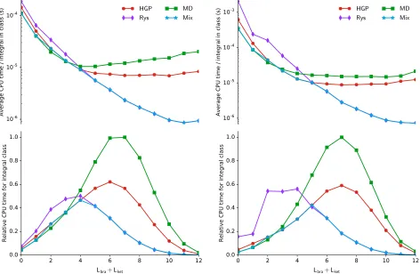
In Figure 2, integral timings are presented for calculations on the small paramagnetic molecule O2. These calculations were
left–hand panel of Figure 2 shows the timings pertaining to the primitive basis set, whilst the right–hand panel shows the corresponding data for the contracted basis set.
In the presence of a strong magnetic field, the electron density of the system is compressed in an anisotropic manner, with the compres-sion perpendicular to the field being more pro-nounced than that in the direction of the ap-plied field, as described for example in Refs. 4,10,11. These changes are however small rel-ative to the changes in density upon formation of a typical covalent bond and so a simple ap-proach to introduce sufficient flexibility into the basis set to adequately accommodate these ef-fects is to un–contract the basis functions. The development of basis sets tailored to finite field calculations has not yet been pursued, however for such sets, contracted functions could be de-veloped to enhance computational efficiency. In Figure 2 we also therefore present timings for the aug-cc-pCVTZ basis set in its contracted form, where the contractions used are those de-fined for zero–field calculations.
In this work, we have only considered fields of up to ∼ 1 atomic unit in strength, equivalent to 2350000 Tesla. For the purposes of
check-ing the numerical stability of the implemented code, some additional calculations were under-taken with fields of up to ∼ 3 atomic units in strength. We note however that, at field strengths greater than a few atomic units, the use of anisotropic basis sets may become nec-essary,57,58 along with a more careful
consider-ation of non Born–Oppenheimer corrections.59
The timings for the primitive basis for O2 in
the left hand panels of Figure 2 are classified by the total angular momentum of the shell quar-tet, Lbra+Lket. In the upper panel, the average
CPU time per integral in each class is presented; this gives a system independent measure of the performance of each algorithm for the different classes of integral. As would be expected from subsection 4.1, the MD algorithm exhibits the least favourable performance overall. The time per integral for the MD algorithm is little dif-ferent from that of the HGP algorithm for very low angular momenta of .2, perhaps having a
marginal advantage over HGP for these classes, however the time per integral for MD rapidly begins to exceed that of HGP for classes of in-creasing angular momenta. This is a result of the recursion relation of Eq. (41) having twice the number of terms and indices as its zero–field counterpart, effectively eliminating a principle advantage of the MD algorithm whilst retain-ing the principle disadvantage in the form of Eq. (42), leading to the relatively poor scaling with angular momentum observed here.
The HGP algorithm delivers a superior per-formance to the MD algorithm for integrals of angular momenta above the range . 2. This is unsurprising because, whilst the VRR of Eq. (44) has one term more than the MD recur-sion relation, the HRR of Eq. (7) is much sim-pler than the transformation stage of the MD algorithm, Eq. (42). In essence, the HGP al-gorithm for LAO-ERIs is little different to that over standard GTOs, thus retains many of its well documented comparative advantages.28,60
momen-0 2 4 6 8 10 12
Lbra+Lket
0.0 0.2 0.4 0.6 0.8 1.0
Relative CPU time for integral class
10-6
10-5
10-4
Average CPU time / integral in class (s)
HGP Rys
MD Mix
0 2 4 6 8 10 12
Lbra+Lket
0.0 0.2 0.4 0.6 0.8 1.0
Relative CPU time for integral class
10-6
10-5
10-4
10-3
Average CPU time / integral in class (s)
HGP Rys
[image:15.612.71.543.44.352.2]MD Mix
Figure 2: Relative timings for LAO-ERIs in a calculation on the O2 molecule in the aug-cc-pCVTZ
basis, classified according to the total angular momenta Lbra+Lket for each shell quartet. The left
hand panels show the results for the primitive basis, the right hand panels for the contracted basis set.
tum, being in this case inferior to both MD and HGP. This is because the zeroth–order terms of the MD and HGP algorithms are simply scaled molecular incomplete gamma functions and are relatively inexpensive to compute, whereas the zeroth–order terms of the Rys algorithm re-quires the more computationally expensive cal-culation of quadrature nodes and weights. For integrals of low angular momentum, comput-ing the zeroth–order term is generally the dom-inant step, thus the pre–factor is greater for the Rys quadrature than for the MD or HGP algo-rithms, impairing the performance of the Rys scheme at low angular momenta.
In the lower panel of Figure 2, the relative CPU time for each integral class in the calcula-tion is presented; this plot reflects not only the angular momenta of integrals present but also their relative distribution as determined by the particular choice of basis and the system under study. It is again clear that he MD approach
is the least efficient, with the largest amount of time spent on integrals withLbra+Lket= 7, the
HGP algorithm delivers a considerable improve-ment forLbra+Lket >4, and is comparable with
MD for lower angular momenta integrals. For the HGP approach, the most time is spent on integrals with Lbra+Lket = 6. Most striking is
the significant improvement offered by the use of Rys quadrature forLbra+Lket >4, with the
largest amount of time being spent on integrals withLbra+Lket = 4 for this approach.
Further-more, as would be anticipated from the above discussion, forLbra+Lket <4 the Rys approach
is noticeably less efficient than either the MD or HGP schemes.
particularly efficient for contracted basis sets since its HRR may be applied to contracted in-tegrals. This effect can be discerned in the up-per right plot of Figure 2, noting that the HGP algorithm becomes more efficient than MD ear-lier at Lbra +Lket = 2. On the other hand,
the efficiency of the Rys quadrature calcula-tions is adversely effected by contraction, as it necessitates multiple sets of quadrature roots and weights to be computed per integral batch; this effect can be discerned from the upper right plot, noting a later crossover with HGP at
Lbra+Lket = 5, beyond which the Rys
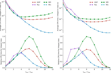
quadra-ture again becomes the most efficient technique. A similar analysis has been conducted for the cyclobutadiene molecule, C4H4, at the same
ge-ometry as used in Ref. 1 with a uniform mag-netic field of strength 1 atomic unit perpendic-ular to the molecperpendic-ular plane. The results per-taining to the C4H4 molecule are presented in
Figure 3. The upper panels showing the sys-tem independent plots are remarkably similar to those for O2, confirming the use of this
mea-sure for assessing the efficiency of the different algorithms. In particular, the crossover values at which different methods become the most ef-ficient are remarkably transferrable. The lower panels are also very similar, reflecting similar types of functions contributing to the basis set. We have confirmed that increasing the cardi-nal number of the Dunning-type basis set does not significantly affect conclusions on the rela-tive efficiency of the approaches considered and that the system independent plots (upper pan-els) remain broadly system independent.
Given that the crossovers in performance be-tween the algorithms are remarkably trans-ferrable, we have considered a simple mixed ap-proach to achieve the optimal efficiency in eval-uating the LAO-ERIs. In all constituent plots of Figures 2 and 3, the results of the mixed ap-proach are plotted with line style ?−?. In our integral evaluation code, we have introduced a simple function to select the most appropri-ate algorithm based on the overall contraction length and the value of Lbra+Lket. After
test-ing over a range of systems we select the MD, HGP and Rys algorithms based on these val-ues according to Table 1. This approach can
Table 1: Ranges of Lbra +Lket in which each
of the considered integral algorithms may be considered optimal. These values are used for the construction of a mixed scheme (see text for details).
MD HGP Rys Primitive 0–1 2–4 5+ Contracted 0–1 2–5 6+
be highly effective in reducing overall compu-tation time, compared with the exclusive use of any one of the algorithms, often with sav-ings between 10% and 30%. The largest gains using the mixed approach are apparent when using contracted functions (see e.g. the lower right panels of Figures 2 and 3). It is inter-esting to note that all three approaches con-sidered contribute to the mixed scheme, with MD being most efficient for the lowest angular momenta integrals, Rys quadrature the most efficient for the high angular moment integrals and HGP being optimal in the intermediate re-gion. We expect the simple heuristics used in the mixed approach here to be transferrable to many common basis sets where contraction is most significant in the lower angular momenta core functions. However, some re–calibration may of course be necessary for basis sets taining functions with significantly greater con-traction lengths than tested in this work.
6
Conclusions
0 2 4 6 8 10 12
Lbra+Lket
0.0 0.2 0.4 0.6 0.8 1.0
Relative CPU time for integral class
10-6
10-5
10-4
Average CPU time / integral in class (s)
HGP Rys
MD Mix
0 2 4 6 8 10 12
Lbra+Lket
0.0 0.2 0.4 0.6 0.8 1.0
Relative CPU time for integral class
10-6
10-5
10-4
Average CPU time / integral in class (s)
HGP Rys
[image:17.612.71.542.44.352.2]MD Mix
Figure 3: Relative timings for LAO-ERIs in a calculation on the C4H4 molecule in the
aug-cc-pCVTZ basis, classified according to the total angular momenta Lbra+Lket for each shell quartet.
The left hand panels show the results for the primitive basis, the right hand panels for the contracted basis set.
of LAOs does not significantly complicate the underlying algorithm and the efficiency of the HGP scheme for contracted basis functions re-mains a significant advantage in the generalized form.
For the Rys quadrature approach, a careful approach is required to extend the method to the complex case required for LAO integrals. In contrast with previous implementations, we use Flocke’s approach27 rather than an
interpola-tion scheme for the roots and weights, avoiding the need to construct and store large interpo-lation tables.8 We also find that the
compu-tation of the roots and weights on the fly can be carried out with standard double precision arithmetic. The reduced multiplication scheme of Lindh52 was adopted in this context to
fur-ther improve the efficiency of the summation step. One potential complicating factor for the application of Rys quadrature in this context is the possibility of encountering singularities
in the complex plane.8,47 Whilst we have
con-firmed that these are still present with use of the alternative algorithms presented here, we have not encountered difficulties due to these in any practical calculations, including tests with molecules at a wide range of geometries with fields up to 3 atomic units in strength. In our implementation, if such problems are detected the evaluation of the integral batch can be re-peated automatically with a larger number of roots and weights or with one of the alternative LAO-ERI algorithms.
approach can achieve substantial efficiencies in overall computation compared with the exclu-sive use of any one integral algorithm. This provides a robust approach for calculating LAO molecular integrals over a very broad range of fields in an efficient manner, enabling the effi-cient implementation of non-perturbative treat-ments of strong magnetic fields in electronic structure calculations. In future work, we will consider the evaluation of geometrical deriva-tives of these integrals in a similar fashion to enable the efficient calculation of molecular gra-dients and optimized geometries in the presence of strong magnetic fields.
Acknowledgements
The authors are grateful for support from the Engineering and Physical Sciences Research Council (EPSRC), Grant No. EP/M029131/1. AMT gratefully acknowledges support from the Royal Society University Research Fellowship scheme.
References
(1) Tellgren, E. I.; Soncini, A.; Helgaker, T. Nonperturbative ab initio calculations in strong magnetic fields using London or-bitals.J. Chem. Phys. 2008,129, 154114.
(2) Tellgren, E. I.; Helgaker, T.; Soncini, A. Non-perturbative magnetic phenomena in closed-shell paramagnetic molecules.
Phys. Chem. Chem. Phys.2009,11, 5489.
(3) Tellgren, E. I.; Reine, S. S.; Helgaker, T. Analytical GIAO and hybrid-basis inte-gral derivatives: application to geome-try optimization of molecules in strong magnetic fields.Phys. Chem. Chem. Phys. 2012, 14, 9492.
(4) Lange, K. K.; Tellgren, E. I.; Hoff-mann, M. R.; Helgaker, T. A Paramag-netic Bonding Mechanism for Diatomics in Strong Magnetic Fields. Science 2012,
337, 327–331.
(5) Tellgren, E. I.; Fliegl, H. Non-perturbative treatment of molecules in linear magnetic fields: Calculation of anapole susceptibili-ties. J. Chem. Phys. 2013, 139, 164118.
(6) Tellgren, E. I.; Teale, A. M.; Fur-ness, J. W.; Lange, K. K.; Ekstr¨om, U.; Helgaker, T. Non-perturbative calcula-tion of molecular magnetic properties within current-density functional theory.
J. Chem. Phys. 2014, 140, 034101.
(7) Reimann, S.; Ekstr¨om, U.; Stopkow-icz, S.; Teale, A. M.; Borgoo, A.; Hel-gaker, T. The importance of current contributions to shielding constants in density-functional theory. Phys. Chem. Chem. Phys. 2015, 17, 18834–18842.
(8) Reynolds, R. D.; Shiozaki, T. Fully rela-tivistic self-consistent field under a mag-netic field. Phys. Chem. Chem. Phys. 2015,17, 14280–14283.
(9) Stopkowicz, S.; Gauss, J.; Lange, K. K.; Tellgren, E. I.; Helgaker, T. Coupled-cluster theory for atoms and molecules in strong magnetic fields. J. Chem. Phys. 2015,143, 074110.
(10) Furness, J. W.; Verbeke, J.; Tellgren, E. I.; Stopkowicz, S.; Ekstr¨om, U.; Helgaker, T.; Teale, A. M. Current Density Functional Theory Using Meta-Generalized Gradi-ent Exchange-Correlation Functionals. J. Chem. Theory Comput. 2015, 11, 4169– 4181.
(11) Furness, J. W.; Ekstr¨om, U.; Helgaker, T.; Teale, A. M. Electron localisation function in current-density-functional theory. Mol. Phys. 2016, 114, 1415–1422.
(12) Hampe, F.; Stopkowicz, S. Equation-of-motion coupled-cluster methods for atoms and molecules in strong magnetic fields.J. Chem. Phys. 2017, 146, 154105.
(14) Ditchfield, R. Self-consistent perturbation theory of diamagnetism.Mol. Phys.1974,
27, 789–807.
(15) Obara, S.; Saika, A. Efficient recursive computation of molecular integrals over Cartesian Gaussian functions. J. Chem. Phys. 1986, 84, 3963.
(16) Honda, M.; Sato, K.; Obara, S. Formula-tion of molecular integrals over Gaussian functions treatable by both the Laplace and Fourier transforms of spatial opera-tors by using derivative of Fourier-kernel multiplied Gaussians. J. Chem. Phys. 1991, 94, 3790.
(17) Kiribayashi, S.; Kobayashi, T.; Nakano, M.; Yamaguchi, K. Self-consistent-field calculations of molecular magnetic properties using gauge-invariant atomic orbitals. Int. J. Comput. Theor. Chem. 1999,75, 637–643.
(18) Ishida, K. ACE algorithm for the rapid evaluation of the electron-repulsion inte-gral over Gaussian-type orbitals. Int. J. Comput. Theor. Chem. 1996, 59, 209– 218.
(19) Ishida, K. Molecular integrals over the gauge-including atomic orbitals.J. Chem. Phys. 2003, 118, 4819.
(20) Dupuis, M. Evaluation of molecular in-tegrals over Gaussian basis functions. J. Chem. Phys.1976, 65, 111.
(21) King, H. F.; Dupuis, M. Numerical inte-gration using rys polynomials.J. Comput. Phys. 1976, 21, 144–165.
(22) McMurchie, L. E.; Davidson, E. R. One-and two-electron integrals over carte-sian gauscarte-sian functions.J. Comput. Phys. 1978, 26, 218–231.
(23) Tachikawa, M.; Shiga, M. Evaluation of atomic integrals for hybrid Gaussian type and plane-wave basis functions via the McMurchie-Davidson recursion formula.
Phys. Rev. E 2001, 64, 056706.
(24) Kuchitsu, T.; Okuda, J.; Tachikawa, M. Evaluation of molecular integral of Carte-sian GausCarte-sian type basis function with complvalued center coordinates and ex-ponent via the McMurchie-Davidson re-cursion formula, and its application to electron dynamics.Int. J. Comput. Theor. Chem. 2009,109, 540–548.
(25) LONDON, A quantum chemistry pro-gram for plane–wave/GTO hybrid basis sets and finite magnetic field calculations.
londonprogram.org.
(26) BAGEL, Brilliantly Advanced General Electronic-structure Library. nubakery. org, Published under the GNU General Public License.
(27) Flocke, N. On the use of shifted Ja-cobi polynomials in accurate evaluation of roots and weights of Rys polynomials. J. Chem. Phys. 2009, 131, 064107.
(28) Gill, P. M.Adv. Quantum Chem.; Elsevier BV, 1994; pp 141–205.
(29) Gill, P. M. W.; Johnson, B. G.; Pople, J. A.; Taylor, S. W. Modeling the potential of a charge distribution. J. Chem. Phys. 1992, 96, 7178–7179.
(30) Head-Gordon, M.; Pople, J. A. A method for two–electron Gaussian integral and in-tegral derivative evaluation using recur-rence relations. J. Chem. Phys. 1988, 89, 5777.
(31) Rys, J.; Dupuis, M.; King, H. F. Compu-tation of electron repulsion integrals using the Rys quadrature method. J. Comput. Chem. 1983,4, 154–157.
(32) Johnson, B. G.; Gill, P. M.; Pople, J. The efficient transformation of (m0|n0) to (ab|cd) two-electron repulsion integrals.
Chem. Phys. Lett. 1993, 206, 229–238.
Int. J. Comput. Theor. Chem.2006,107, 30–36.
(34) Ryu, U.; Lee, Y. S.; Lindh, R. An effi-cient method of implementing the hori-zontal recurrence relation in the evalua-tion of electron repulsion integrals using Cartesian Gaussian functios.Chem. Phys. Lett. 1991, 185, 562–568.
(35) Schlegel, H. B.; Frisch, M. J. Transforma-tion between Cartesian and pure Spheri-cal harmonic Gaussians. Int. J. Comput. Theor. Chem. 1995, 54, 83–87.
(36) Obara, S.; Saika, A. General recur-rence formulas for molecular integrals over Cartesian Gaussian functions. J. Chem. Phys. 1988, 89, 1540.
(37) Shavitt, I. In Methods Comput. Phys.; Alder, B., Fernbach, S., Rotenberg, M., Eds.; Academic Press New York, 1963; Vol. 3; pp 1–45.
(38) Saunders, V. R. Computational Tech-niques in Quantum Chemistry and Molec-ular Physics; Springer Netherlands, 1975; pp 347–424.
(39) Boys, S. F. Electronic Wave Functions. I. A General Method of Calculation for the Stationary States of Any Molecular Sys-tem. Proc. R. Soc. A1950,200, 542–554.
(40) Helgaker, T.; Jørgensen, P.; Olsen, J.
Molecular Electronic-Structure Theory; John Wiley & Sons, Ltd, 2000.
(41) ˇC´arsky, P.; Pol´aˇsek, M. Incomplete Gam-maFm(x) Functions for Real Negative and Complex Arguments. J. Comput. Phys. 1998, 143, 259–265.
(42) Mathar, R. J. Numerical Representa-tions of the Incomplete Gamma Function of Complex-Valued Argument. Numerical Algorithms 2004, 36, 247–264.
(43) Ishida, K. Accurate and fast algorithm of the molecular incomplete gamma func-tion with a complex argument.J. Comput. Chem. 2004,25, 739–748.
(44) Colle, R.; Fortunelli, A.; Simonucci, S. A mixed basis set of plane waves and Her-mite Gaussian functions. Analytic expres-sions of prototype integrals. Il Nuovo Ci-mento D 1987,9, 969–977.
(45) Colle, R.; Fortunelli, A.; Simonucci, S. Hermite Gaussian functions modulated by plane waves: a general basis set for bound and continuum states. Il Nuovo Cimento D 1988, 10, 805–818.
(46) Golub, G. H.; Welsch, J. H. Calculation of Gauss quadrature rules.Mathematics of Computation 1969, 23, 221–221.
(47) Saylor, P. E.; Smolarski, D. C. Numerical Algorithms 2001, 26, 251–280.
(48) Wilf, H. S. Mathematics for the physical sciences; John Wiley and Sons Inc, 1962.
(49) Sack, R. A.; Donovan, A. F. An algorithm for Gaussian quadrature given modified moments. Numerische Mathematik 1971,
18, 465–478.
(50) Horn, R. A.; Johnson, C. R. Matrix anal-ysis; Cambridge University Press, 1985.
(51) Dongarra, J. J.; Demmel, J. W.; Os-trouchov, S. Computational Statistics; Physica-Verlag HD, 1992; pp 23–28.
(52) Lindh, R.; Ryu, U.; Liu, B. The reduced multiplication scheme of the Rys quadra-ture and new recurrence relations for aux-iliary function based two-electron inte-gral evaluation. J. Chem. Phys.1991,95, 5889.
(53) QUEST, A rapid development platform for Quantum Electronic Structure Tech-niques. 2017.
(54) Numba. numba.pydata.org, 2017;
Ver-sion 0.32.
(56) Kendall, R. A.; Dunning, T. H.; Harri-son, R. J. Electron affinities of the first-row atoms revisited. Systematic basis sets and wave functions.J. Chem. Phys.1992,
96, 6796–6806.
(57) Schmelcher, P.; Cederbaum, L. S. Molecules in strong magnetic fields: Properties of atomic orbitals. Phys. Rev. A 1988, 37, 672–681.
(58) Kubo, A. The Hydrogen Molecule in Strong Magnetic Fields: Optimizations of Anisotropic Gaussian Basis Sets. J. Phys. Chem. A 2007, 111, 5572–5581.
(59) Adamowicz, L.; Tellgren, E. I.; Hel-gaker, T. Non-Born–Oppenheimer calcu-lations of the HD molecule in a strong magnetic field. Chem. Phys. Lett. 2015,
639, 295–299.
(60) Gill, P. M. W.; Pople, J. A. The PRISM algorithm for two–electron integrals. Int. J. Comput. Theor. Chem. 1991, 40, 753– 772.
TOC Graphic
For table of contents only.
MD
HGP
Rys
(ab|cd)ωa∗(r1)ωb(r1)
ω∗c(r2)ωd(r2)
L?
London Atomic Orbital: ωa(r) =φa(r)e−ika·r
Lbra+Lket
t
(
s