Hector Gomez
1, Kristoffer G. van der Zee
2 — 16 Oct. 2015 —1Departamento de M´etodos Matem´aticos, Universidade da Coru˜na, Campus de A Coru˜na, 15071, A Coru˜na, Spain.
2 School of Mathematical Sciences, The University of Nottingham, University Park, Nottingham NG7 2RD, United Kingdom
ABSTRACT
Phase-field modeling is emerging as a promising tool for the treatment of problems with interfaces. The classical description of interface problems requires the numerical solution of partial differential equations on moving domains in which the domain motions are also unknowns. The computational treatment of these problems requires moving meshes and is very difficult when the moving domains undergo topological changes. Phase-field modeling may be understood as a methodology to reformulate interface problems as equations posed on fixed domains. In some cases, the phase-field model may be shown to converge to the moving-boundary problem as a regularization parameter tends to zero, which shows the mathematical soundness of the approach. However, this is only part of the story because phase-field models do not need to have a moving-boundary problem associated and can be rigorously derived from classical thermomechanics. In this context, the distinguishing feature is that constitutive models depend on the variational derivative of the free energy. In all, phase-field models open the opportunity for the efficient treatment of outstanding problems in computational mechanics, such as, the interaction of a large number of cracks in three dimensions, cavitation, film and nucleate boiling, tumor growth or fully three-dimensional air-water flows with surface tension. In addition, phase-field models bring a new set of challenges for numerical discretization that will excite the computational mechanics community.
key words: Phase-field modeling, Thermomechanics, Thermodynamically-consistent algorithms, Isogeometric analysis, Multiphase flows, Fracture mechanics, Tumor growth, Cahn-Hilliard equation.
1. Introduction
1.1. Phase-field modeling in computational mechanics
There are many areas of research in computational mechanics that involve moving boundary problems. Prime examples are fluid-structure interaction, fully three-dimensional air-water flows and crack propagation. The mathematical formulation of these problems often involves partial-differential equations (PDEs) which are posed on moving domains and coupled to another set of PDEs through boundary conditions which hold on a moving and unknown interface. Although in some cases, such as for example, fluid-structure interaction, these problems have been attacked computationally with significant success (Bazilevs et al., 2013; Farhat, 2004), most of them remain as outstanding problems, especially in complicated three-dimensional geometries.
The phase-field method (Emmerich., 2003; Provatas and Elder, 2010; Chen, 2002; Anderson et al., 1998) may be understood as a mathematical theory to reformulate moving boundary problems as PDEs which hold on a known and fixed computational domain. The usual way to achieve this is to introduce a new field, namely, the phase field, which is defined on the entire domain and is a marker of the location of the different phases1. The phase field is governed by an equation
that naturally develops internal layers which mimic the interfaces of the original moving boundary problem. The crucial difference, however, is that the phase field is smooth and, as a consequence, the interfaces have a small but finite width, which is usually controlled by a length scale parameter in the model. For this reason, phase-field models are also called diffuse-interface models and, in contrast, the corresponding moving boundary problems are referred to assharp-interfacetheories. In some cases, the easiest way to derive a phase-field model is to start from a moving boundary problem and smooth it out as described before to obtain its phase-field analogue. This is exactly the approach we take in Sect. 2. The process of smoothing out ordiffusifying2the original problem can be made mathematically rigorous and in some cases the phase-field model may be shown to converge to the moving boundary problem as a regularization parameter that controls the thickness of the interfaces goes to zero. The enabling mathematical technique to prove the convergence of the phase-field model to the sharp-interface equation is the theory of matched asymptotic expansions
(Caginalp, 1989; Fife, 1988).
The diffusification procedure we just sketched, however, is only a small part of the picture. Phase-field models may also be understood in different ways and do not need to have a free-boundary problem associated. They can be derived directly from free-energy functionals using the classical theory of thermomechanics and Coleman-Noll-type approaches (Coleman and Noll, 1963; Truesdell and Noll, 1965). This is the point of view that we adopt in Sect. 3 and the key feature of phase-field models in this context is that constitutive equations are allowed to depend on the variational derivative of the free-energy itself. Using this framework, we derive the classical Allen-Cahn and Cahn-Hilliard models, a theory of two-component immiscible fluids with surface tension, a phase-field model of brittle fracture, a mechano-biological model of tumor growth, and the Navier-Stokes-Korteweg equations which govern liquid-vapor phase transformations.
Regardless of the interpretation that we take, the phase-field method produces models in which interface tracking is avoided, significantly simplifying the numerics. However, the computational treatment of phase-field equations is far from trivial and introduces a new set of challenges for the computational mechanics community. For example, the diffuse interfaces which travel through a fixed computational domain manifest themselves as layers in the solution represented by large gradients of the phase field. Of course, these features of the solution need to be resolved by the computational mesh, which ideally should follow them dynamically. Another important aspect is that in many cases, phase-field theories are governed by fourth- (or higher-) order PDEs. Classical numerical methodologies, such as, for example, the finite-difference method or pseudo-spectral collocation may be used to solve higher-order PDEs on simple geometries (Trefethen, 2000; Axelsson, 2004; Canuto and Quarteroni, 2004). When geometrical flexibility is needed, the finite element method is usually the technique of choice, but solving higher-order PDEs in primal form (i.e., without introducing auxiliary variables representing derivatives of the unknown) in complicated three-dimensional geometries is still an open problem. The difficulty stems from the fact that a standard finite element method requiresCm−1-continuous basis functions to solve a PDE
of order 2m. This requirement may be easily satisfied using the isoparametric concept for PDEs of second order (m= 1), but it is difficult to achieve in complicated three-dimensional geometries for higher-order PDEs (m >1). However, a new technology called isogeometric analysis (Hughes et al., 2005; Cottrell et al., 2009; Aaa, 201xa,x) has recently been introduced in computational mechanics. Isogeometric analysis permits generating basis functions with tailorable global continuity on non-trivial geometries. This, together with the increased robustness of higher-order elements, has opened the way to more efficient algorithms for phase-field models on engineering geometries.
Another computational challenge of phase-field models is time integration (Hairer et al., 1987; Hughes, 2012). Phase-field theories usually derive from non-convex potentials which locally produce the ‘backwards’ diffusion (also referred to as ‘uphill’ diffusion) that gives rise to the natural
propagation problem. The battery of phase-field theories that we show in the paper will hopefully make clear the meaning as the reader advances in the text.
formation of layers in the solution. Mathematically, the equations remain well posed, because they are regularized by higher-order operators, but usual time integration schemes may be inadequate. Sect. 4 treats in detail time integration algorithms for phase-field models, focusing both on accuracy and stability.
In all, we feel that the theoretical and computational developments of the last few years have elevated phase-field modeling to a point in which it can be used as a predictive model for a number of problems in computational mechanics which were very difficult to treat with conventional methodologies. Among these problems, we include the interaction of a large number of cracks in three-dimensional solids of complicated geometry (Borden et al., 2014), fully three-dimensional air-water flows with surface tension (Ceniceros et al., 2010), liquid-vapor phase transitions and cavitation (Liu et al., 2013), nucleate and film boiling (Liu et al., 2015), phase-change-driven implosion of thin structures (Bueno et al., 2014), cellular migration (Shao et al., 2012) and tumor growth (Hawkins-Daarud et al., 2012; Vilanova et al., 2013, 2014, 2012; Xu et al., 2015; Lorenzo et al., 2015) and others (Cueto-Felgueroso and Juanes, 2012, 2014; Gomez et al., 2013). However, even though the last few years witnessed very significant advances in the area, there are still many challenges ahead. Among these challenges, we identify multiphysics and coupled problems, nonlocal phase-field models, and an efficient treatment of randomness and uncertainty in phase-field theories. We have organized the contents of this encyclopedic chapter as follows. Following a short subsection on notational conventions, we consider in Sect. 2 the heuristic derivation of phase-field models via diffusification of moving-boundary problems in the context of solidification. Then in Sect. 3, we consider phase-field models from a thermomechanical perspective, and we derive a variety of phase-field models that are encountered in computational mechanics. In Sect. 4 we consider various time-integration methods, and in Sect. 5 we summarize methods for the spatial discretization of phase-field models. Finally, Sect. 6 contains numerical examples.
1.2. Notational conventions
Let f :I ⊂R7→Rbe a real-valued function defined over a real, open interval I. The functionf
transformsx∈Iintof(x). We denote the derivative off asf0. Alternatively, we will also use the notation ddfx. When we work on several space dimensions, we will employ the notation Ω⊂Rnd to
denote an open subset ofRnd, wheren
dis the number of spatial dimensions. In this paper,nd= 3 in most cases, but there are subsections in whichnd= 2 ornd= 1. The closure of Ω is denoted by Ω and its boundary by∂Ω. The set∂Ω is supposed to have a well-defined unit outward normal. A spatial point x∈Ω is represented in component notation as x= (x1, x2, . . . , xnd)
T. Throughout the manuscript, the variablet∈R+∪ {0}denotes time. We often use functions which depend upon
space and time, for example φ: Ω×[0, T]7→R, where [0, T] is the time interval of interest. The
partial derivatives ofφare interchangeably denoted as
∂iφ=
∂φ ∂xi
, ∂tφ=
∂φ
∂t (1)
We also make use of standard notation based on the operator ∇. For example, ∇φ denotes the spatial gradient of φ. We often resort to the use of material time derivatives as defined, e.g., in (Marsden and Hughes, 1994). For example, ˙φdenotes the material derivative of φ which may be interpreted as a derivative with respect to time holding a material particle fixed. For a velocity field u, we have ˙φ=∂tφ+u·∇φ. Throughout the manuscript, we also utilize functions which are defined on sets of material points, rather than spatial points. Material points are also called particles and we denote them by X. For functions defined on sets of particles, material time derivatives are simply regular partial derivatives with respect to time. Sets of particles are denoted as Ω0 or P0.
The spatial position of a set of particles at timetis usually denotedPt. Volumetric integrals defined on sets of spatial points are usually denoted R
Ωdx, while for surface integrals we use the notation
R
∂Ωda. When the integrals are defined on sets of material points, we use the notation
R
Ω0dX and
R
∂Ω0dA.
The reader should also keep in mind that this paper describes a number of phase-field theories using the thermomechanics framework. Many of these theories involve, for example, Cauchy stress
tensors, which are usually denoted T. The reader should not understand thatT denotes exactly the same quantity throughout the manuscript. Rather, T denotes the Cauchy stress tensor of a particular mechanical theory ans its precise definition may vary from one section to another. This situation is not specific to T and happens also with other quantities such as, for example, the Helmholtz free energy Ψ, the mass fluxh, the phase fieldφ, the reaction termR, the dissipationD and others. The precise definition is made clear in each subsection such that no confusion arises.
2. From classical moving-boundary problems to phase-field models via diffusification
In this section we show how classical problems involving moving boundaries and interfaces can be
regularized and written as PDEs posed on a fixed domain using the theory of phase-field modeling. The regularization replaces sharp interfaces bydiffuse interfaces that are described with the help of the phase-field variable. As indicated before, we shall refer to this particular type of regularization as diffusification.
We consider the classical solidification theory for pure materials, also known as the generalized Stefan problem. The classical formulation consists of two PDEs which hold on different, but adjacent, time-dependent domains. The PDEs are coupled through conditions on the interface, whose location changes with time and is a priori unknown. We demonstrate heuristically how to
diffusify this moving-boundary problem and obtain a phase-field model of solidification, which is a PDE system on afixed domain.
2.1. Moving-boundary problem for solidification: The generalized Stefan problem
Let us consider a solid-liquid system that may undergo phase transformations. The system occupies the spatial domain Ω, which is fixed in time. The set Ω can be decomposed as Ω = ΩS∪ΩL, where ΩS and ΩLare the regions of Ω that host the solid and liquid phase, respectively. The sets ΩS and ΩL change with time, and their motions are unknowns of the problem. The solid-liquid interface, which is located where ΩS and ΩL meet is denoted ΓLS. Omitting the boundary conditions on∂Ω for simplicity, the classical sharp-interface theory is described by the following equations
∂e
∂t + divq= 0 in ΩS∪ΩL (2)
λVn =−JqK·nLS on ΓLS (3)
JθK= 0 on ΓLS (4)
ωVn+σκ=λ(θ−θm) on ΓLS (5)
The system composed by Eqs. (2)–(5) is known as the generalized Stefan problem3. Eqns. (2) and
(3) correspond to the energy balance for a body with discontinuous material properties, (4) simply reflects that the temperature is continuous across the solid–liquid interface, and (5) is the so-called
Gibbs-Thomson condition that determines the motion of the interface. In Eq. (2),eis the internal energy and q is the heat flux. Importantly, both eand q are discontinuous across the solid-fluid interface ΓLS due to the phase change. The internal energy is defined as
e=Cvθ+λχS (6)
whereCvis the heat capacity,θis the temperature,λis the latent heat, andχS is the characteristic function of ΩS, that is, a function defined on Ω that takes the value 0 in ΩL and 1 in ΩS. The heat flux is assumed to be governed by Fourier’s law4, that is, q = −k∇θ, where the conductivity k
equals the value kS in ΩS and the (possibly distinct) valuekL in ΩL. In Eq. (3),nLS is the unit normal to ΓLSpointing towards the solid,Vnis the normal velocity of the interface in the direction
of nLS and the operatorJ·K denotes the jump across ΓLS such thatJqK=qS−qL. In Eq. (5),ω is the coefficient of kinetic undercooling,σis the surface tension of the liquid-solid interface,θmis the melting temperature, andκis the sum of principal curvatures of ΓLS(with the sign convention that κis positive for liquid spherical bubbles).
2.2. The idea behind diffusification
In the above sharp-interface theory, we have three conditions at the interface ΓLS, which may be understood as one boundary condition for ΩS, one boundary condition for ΩL, and another one to determine the interface motion which is unknown a priori. Problem (2)–(5) is thus a moving-boundary problem. Note that in the particular case ω = σ = 0, the Gibbs–Thomson condition becomes θ=θmon ΓLS. In this particular case, the interface can be defined as theθmlevel set of the temperature. However, in the general case in whichωandσare non-zero, additional information is needed to locate the interface. In a phase-field formulation the additional information for the interface location is addressed by introducing a new variable, which is precisely thephase field, and which is nothing else but a marker of the phases’ location. Note that this additional variable isnot
an artifact of the phase-field theory, but it is fundamentally necessary because the temperature is not enough to determine the position of the interface.
Let us proceed to diffusify the sharp-interface theory and obtain the corresponding phase-field model. The key idea is to introduce asmooth field, namely,φ, which is defined on the entire domain Ω = ΩS∪ΩL and which is time-dependent, i.e., φ= φ(x, t). This field will be designed in such a way that it takes approximately the value −1 in the liquid phase, +1 in the solid phase, and it transitions quickly across the normal direction to the interface ΓLS. Let us use as a fundamental hypothesis a hyperbolic tangent profile, therefore
φ(x, t) =f
d
t(x) √
2
:= tanh
d
t(x) √
2
(7)
where dt(x) denotes the signed distance fromxto ΓLS (negative in the liquid and positive in the solid) and is a length scale related to the thickness of the diffuse interface. Note that ΓLS can be identified by the zero level set of φ. The subscript t in dt emphasizes that ΓLS changes with time, but will be removed from now on for notational simplicity. By using assumption (7), we will heuristically derive a phase-field model. Then, we will show that as→0, the ansatz (7) is indeed recovered by the solution of the phase-field model, which gives coherence to the framework.
2.3. Derivation of a phase-field model for solidification
We proceed by suitably diffusifying the equations in (2), (3) and (5). We start with (5) and compute the geometric terms using the phase field φ.
From basic geometry, it is known that|∇d|= 1,nLS=∇dat ΓLS, and the curvature tensorκ satisfies κ=∇∇dat ΓLS; see, e.g., (Deckelnick et al., 2005). From Eq. (7), one can compute the spatial derivatives
∂iφ= 1 √
2f
0√d
2
∂id (8)
∂ij2φ= 1 22f
00√d
2
∂id∂jd+ 1 √
2f
0√d
2
∂ij2d (9)
Using the hyperbolic-tangent identitiesf0= 1−f2, andf00=−2f f0, we then obtain the curvature tensor in terms ofφ:
κij =∂ij2d= √
2
1−φ2
∂ij2φ+ 2φ
1−φ2∂iφ∂jφ
(10)
The additive curvature, defined asκ= ∆d, can then be written as
κ=
√ 2
(1−φ2)
∆φ+ 2φ 1−φ2|∇φ|
2
(11)
Next, using again the relation f0= 1−f2, it may be shown that
2
2|∇φ|
2=1
4(1−φ
2)2 (12)
Let us introduce at this point the function
W(φ) =1 4(1−φ
2)2 (13)
referred to as a double-well potential. The key feature of the function W is that it has two local minima which makes possible the coexistence of solid and liquid phases. Using the expression ofW, we obtain
κ= −
√ 2 (1−φ2)
W0(φ)
−∆φ
(14)
We will now compute the normal velocity of ΓLS, which is given by the zero level set ofφ. Let rLS(t) be a position vector that points to a material particle of the interface ΓLS, and define the functionφe(t) =φ(rLS(t), t). The functionφeis identically zero by definition of ΓLS. Therefore, its derivative is also identically zero. Using the chain rule, we obtain
0 =φe0=∇φ·
drLS
dt +∂tφ (15)
If we use the notation vLS= drLS/dt, we can rewrite (15) as
∂tφ+vLS· ∇φ= 0 (16)
which is known as the level set equation (Fedkiw and Osher, 2003; Sethian, 1999). Using Eq. (8), and the definition of nLS, we conclude that
∇φ=√1 2f
0√d
2
nLS (17)
Vn is the velocity normal to ΓLS, that is,Vn=vLS·nLS, thus introducing Eq. (17) into the level set equation, and using thatf0 = 1−f2= 1−φ2, we get
Vn= −√2
1−φ2∂tφ (18)
Substituting (14) and (18) into (5), we have now derived the phase-field equation:
ω σ∂tφ+
W0(φ)
−∆φ
=−√λ
2σ(1−φ
2)(θ−θm) (19)
To obtain a regularized energy equation, we shall now diffusify (2)–(3). We consider smooth test functionsv defined on the entire domain Ω and for whichv= 0 on the external boundary∂Ω. The test functionsv are not necessarily zero on ΓLS, but [[v]] = 0 at ΓLS. We now claim that both (2) and (3) are equivalent to the requirement
d dt
Z
Ω
evdΩ =
Z
Ω
q· ∇vdΩ (20)
for all test functions v. To see this, note that the left-hand side equals
d dt
Z
ΩL∪ΩR
evdΩ =
Z
ΩL∪ΩR
v ∂tedΩ−
Z
ΓLS
[[e]]v VndΓ (21)
by Reynolds’ Theorem, while the right-hand side equals
Z
ΩL∪ΩR
q· ∇vdΩ =
Z
ΩL∪ΩR
−v divqdΩ +
Z
ΓLS
Collecting the interior terms and the interface terms, and noting that [[e]] = λ, reveals the equivalence with (2) and (3).
The final ingredients that we need to diffusify (20) are interpolation functions h(φ) andk(φ), which are required to satisfy h(±1) = 1
2 ± 1
2,k(+1) =kS and k(−1) =kL. The simplest choices
fulfilling these conditions are
h(φ) =12(1 +φ) (23)
k(φ) =12(1 +φ)kS+12(1−φ)kL (24)
Using these interpolations, we approximateeandq by
e=Cvθ+λh(φ) (25)
q=−k(φ)∇θ (26)
With these approximations in mind, eandq are smooth across ΓLS, and Eq. (20) is then simply equivalent to
∂te+ divq= 0 (27)
which, upon substitution, yields the diffusified energy equation
Cv∂tθ+λh0(φ)∂tφ−div k(φ)∇θ
= 0. (28)
The system of equations (19) and (28) completes the phase-field model, which represents an elementary phase-field solidification theory.
2.4. The diffuse-interface transition profile: Asymptotic analysis
Given the phase-field model of solidification, Eqs. (19) and (28), let us verify that it indeed gives rise to diffuse interfaces with the hyperbolic tangent profile (7) as→0. We give a heuristic outline, but this procedure can be formalized using the theory ofmatched asymptotic expansions(Caginalp, 1989; Fife, 1988).
Let us first verify separation into phases on short time-scales. Letτ =t/2 denote a rescaling of
time. Then, Eq. (19) can be written as
−2∂τφ+
σ
ωW
0(φ)=O(−1) as→0. (29)
where we have used Landau notation on the right hand side. For smallthe coefficient in front of the left-hand side is significantly larger than the right-hand side so that
∂τφ≈ −
σ
ωW
0(φ), (30)
which means that φ quickly evolves towards the stable roots φ= ±1 of −W0(φ) = −φ3+φ. In
other words, φquickly separates into phases and generates a diffuse interface between them. Let us denote the zero level set of φ by Γ
LS. It is expected that Γ
LS converges to ΓLS as
→ 0. We next verify the profile of φ in a neighbourhood of Γ
LS. We will zoom in to an O( )-neighbourhood of Γ
LS by considering a change of the independent variables. For simplicity, we consider a two-dimensional problem. We change from the variables (x1, x2) to (z, s), where
z(x1, x2, t;) =
d(x
1, x2, t;)
(31)
is a re-scaling of the signed distance to ΓLS(t) ands(x1, x2, t;) is the arc length of ΓLS(t). Denoting
φ(x1, x2, t) = Φ(z, s, t), then in a neighbourhood of ΓLS:
∂tφ=∂tΦ +−1∂zΦ∂td+∂sΦ∂ts (32)
∆φ=−2∂zzΦ +−1∂zΦ ∆d+∂ssΦ|∇s|2+∂sΦ ∆s (33)
where we have used the identity∇s· ∇d= 0. Substitution into (19) yields:
−2W0(Φ)−∂zzΦ=O(−1), (34)
so that upon neglecting the right-hand side, one obtains, in a neighbourhood of ΓLS,
W0(Φ)−∂zzΦ≈0. (35)
This is a second-order ordinary differential equation subject to the boundary conditions Φ(z)→ ±1 as z→ ±∞. Its solution is the anticipated hyperbolic tangent profile:
Φ(z) = tanh√z
2 = tanh
d
√2 (36)
which was the hypothesis in the derivation of the phase-field model in Sect. 2.2.
3. General framework of thermomechanics and energy dissipation for phase-field models
This section illustrates the rigorous thermomechanical framework of phase-field theories. Our approach to thermomechanics follows closely the classical work of (Truesdell and Noll, 1965). Related work in the context of phase-field models can be found in (Gurtin, 1996) and (Oden et al., 2010). The main idea behind this approach is that theories of mechanics are fundamental balance laws of mass, linear momentum, angular momentum, and energy, while constitutive relations are suitably restricted by demanding that the theory be energy dissipative (or entropy productive). One refers to models derived this way asthermomechanically orthermodynamically consistent.
In the remainder of this section, we derive using the thermomechanics framework, the following models:
• The classical Allen-Cahn and Cahn-Hilliard equations, which may be considered as the two canonical models of non-conserved and conserved phase dynamics,
• The Navier-Stokes-Cahn-Hilliard equations which constitute a model for two-component immiscible flows with surface tension,
• A simple phase-field model of brittle fracture, which is the diffuse version of Griffith’s theory of fracture,
• A phase-field model of tumor growth, which predicts the dynamics of cancerous tumors and nutrients in avascular tissue,
• The thermal Navier-Stokes-Korteweg equations, which are a model for liquid-vapor transformations of a single-component fluid.
Another classical problem in which phase-field modeling is widely used is solidification. A thermomechanics framework may be used to derive solidification models (Wang et al., 1993; Penrose and Fife, 1990), but we do not cover this here because solidification was discussed in Sect. 2 using a different perspective. We remark that thediffusification procedure employed in Sect. 2 does not necessarily lead to thermomechanically-consistent models.
3.1. The idea behind thermomechanically-consistent phase-field modeling
Fundamental to phase-field thermomechanics is the dependence of the Helmholtz free energy Ψ (or entropy) on values and gradients of the phase field φ, and, additionally, the dependence of other constitutive relations on the values and/or gradients of thevariational derivativeof the total energy functional with respect to the phase.
For example, the canonical free energy, which goes back to (Cahn and Hilliard, 1958), depends on the phase φand its gradient ∇φ, and has the form
Ψ =G(φ) +
2
2|∇φ|
for some functionGand parameter. The corresponding energy functional is known as aGinzburg– Landau functional:
F(φ) =Z
Ω
Ψ dx=
Z
Ω
G(φ) +
2
2|∇φ|
2dx (38)
The variational derivative is then
δF
δφ =G
0(φ)−2∆φ (39)
which is used to define the so-called chemical potential µ = δδφF =G0(φ)−2∆φ. In phase-field models, constitutive relations are allowed to depend on µand/or∇µ. This will be worked out in detail for the above-mentioned phase-field models in the following sub-sections.
It is possible to interpret the energy functional F as a diffusification of the surface-energy functional
F(Γint) =ψ
Z
Γint
da (40)
where Γint is an interior surface andψis a surface-energy coefficient. Note thatF(Γint) associates
energy to an interface which is proportional to the length of the interface. The simplest connection is obtained by considering F(φ) and F(Γ
int), where φ is a diffusification of the interface
Γint, such that G(φ) =
2
2|∇φ
|2. For example, in case that G(φ) = W(φ), recall (13), then
φ(x) = tanhdΓint√(x)
2ε , withdΓint the distance function to Γint. Note that this particularφ
satisfies the required identity; see (12). It can then be shown that
lim →0
1
F
(φ) =F(Γ
int) (41)
by employing theco-area formula
lim →0
1
Z
Ω
qdΓint(x)
dx=αq
Z
Γint
da (42)
with constantαq =
R∞
−∞q(z) dz. The co-area formula is valid for suitably decaying functionsq(z),
see (Du et al., 2005, Lemma 2.1). By taking the limit in (41), the parameter ψ can be suitably identified. To sum up, phase-field energies collapse to surface energies as the interface thickness
approaches zero.5
3.2. Allen-Cahn and Cahn-Hilliard
The two canonical phase-field theories are the Allen-Cahn equation and the Cahn-Hilliard equation (Emmerich., 2003; Provatas and Elder, 2010). They both emanate from the Ginzburg–Landau energy functional in Eq. (38), withG(φ) a double-well potential. The most usual approach would be to takeG(φ) =W(φ) = 14(1−φ2)2, but there are other possible choices, such as the logarithmic double well; see Eq. (194). Essentially the Allen-Cahn and Cahn-Hilliard equations are designed in such a way that they are gradient flows for the energy. This means that the energy is time decreasing along solutions to the equations. The Cahn-Hilliard equation incorporates the additional requirement that the mass of the components is conserved, while the Allen-Cahn equation allows for non-conservative dynamics.
The thermomechanical derivation of the Allen-Cahn equation and the Cahn-Hilliard equation starts by defining theconstitutive class6 for Ψ:
Ψ =Ψ(b φ,∇φ) (43)
5A rigorous connection between the functionalsF and F can be made using the key mathematical theory of Γ-convergence (Ambrosio and Tortorelli, 1990; Braides, 2002; Dal Maso, 1993).
Let V ⊂Ω denote an arbitrary part of the spatial domain Ω. The postulated energy-dissipation property may be expressed as
d dt
Z
V
b
Ψ(φ,∇φ)dx
=W(V)− D(V) (44)
where the dissipation D(V) is≥0 for all conceivable processes, whileW(V) denotes theworking, which is associated to external forces or energy supplies coming through the boundary ofV. Basic manipulations on the left hand side of (44) lead to
d dt
Z
V
Ψdx=
Z
V
h
∂φΨb∂tφ+∂∇φΨb·∂t(∇φ) i
dx (45)
Let us now integrate by parts the last term of Eq. (45) after flipping the time and space derivatives. Doing so, we obtain,
d dt
Z
V
Ψdx=
Z
V
µ ∂tφdx+
Z
∂V
∂∇φΨb·n∂tφda (46)
where µis the chemical potential defined as the variational derivative:
µ= δ
δφ
Z
V
b
Ψ dx=∂φΨb−div
∂∇φΨb
(47)
Now, we proceed to derive the Allen-Cahn and the Cahn-Hilliard equations.
3.2.1. Allen-Cahn equation The Allen-Cahn equation can be derived by postulating the mass balance
∂φ
∂t =−R (48)
where Ris designed to achieve free-energy dissipation and assumed to have the dependence:
R=Rb(φ,∇φ, µ) (49)
Note the non-standard dependence of R on the variational derivative of the free energy. This is one of the essential features of the phase-field method. Now, to find restrictions on R, we combine Eqs. (46)–(48), which leads to the expression
d dt
Z
V
Ψdx=
Z
V
−µRdx+
Z
∂V
∂∇φΨb·n∂tφda (50)
Here, we identifyDandWasD(V) =R
VµRdxandW(V) =
R
∂V∂∇φΨb·n∂tφda. The nonstandard work term is caused by internal forces∂∇φΨ conjugate to changes inb φ (Gurtin, 1996). It is clear
that the constitutive choiceRb(φ,∇φ, µ) =m(φ)µwithm(φ)≥0 achieves the required property of
free-energy dissipation. For the classical choice
b
Ψ(φ,∇φ) =W(φ) +
2
2|∇φ|
2 (51)
withW(φ) a double well potential, one has
µ=W0(φ)−2∆φ (52)
and we have thus derived the Allen-Cahn equation:
∂φ
∂t =−m(φ)
3.2.2. Cahn-Hilliard equation We start with a statement of mass conservation7, namely
∂φ
∂t + divh= 0 (53)
where the constitutive class of his given by
h=hb(φ,∇φ, µ,∇µ) (54)
Using again Eq. (46), it follows that
d dt
Z
V
Ψdx=
Z
V
−µdivhdx+
Z
∂V
∂∇φΨb ·n∂tφda (55)
Integrating by parts the first term on the right-hand side, we obtain
d dt
Z
V
Ψdx=
Z
V
h· ∇µdx+
Z
∂V
−µh+∂∇φΨb∂tφ
·nda (56)
where the first term on the right-hand side is identified as −D(V) and the second as W(V). Therefore, the constitutive choice
b
h(φ,∇φ, µ,∇µ) =−m(φ)∇µ with m(φ)≥0 (57)
guarantees free-energy dissipation and leads to the Cahn-Hilliard equation:
∂φ ∂t = div
m(φ)∇ W0(φ)−2∆φ (58)
for the above choice of Ψ. We note thatb µhin Eq. (56) can be interpreted as a free-energy flux.
3.3. Navier-Stokes-Cahn-Hilliard
The Navier-Stokes-Cahn-Hilliard equations represent a model for immiscible two-component fluid flow with surface tension. This theory has been widely studied from the physical, the mathematical and the computational points of view (Gurtin et al., 1996; Jacqmin, 1999; Gal and Grasselli, 2010; Kay et al., 2008; Boyer et al., 2010; Gal and Grasselli, 2011; Lowengrub and Truskinovsky, 1998; Colli et al., 2012; Kim et al., 2004; Liu and Shen, 2003). To derive the theory, let us assume that we have two immiscible components with volume fractions ϕ1 and ϕ2, respectively. The volume
fractions verify the constraint
ϕ1+ϕ2= 1 (59)
The velocities of the components are denotedu1andu2, and their densitiesρ1andρ2. The density
of the mixture, namely,ρis defined asρ=ϕ1ρ1+ϕ2ρ2. The mass-averaged velocity of the mixture
is defined as
u= 1
ρ(ϕ1ρ1u1+ϕ2ρ2u2) (60)
For simplicity, both components of the mixture are supposed to be incompressible with constant density. In addition, we will assume ρ1 =ρ2. Taken together, these assumptions imply that the
mixture density ρis also a constant equal to ρ1 and ρ2. Therefore, without loss of generality, we
can take
ρ=ρ1=ρ2= 1 (61)
In this scenario, mass conservation of the components implies
d dt
Z
Pt
ϕα= 0; α= 1,2 (62)
7Note that Eq. (53) achieves mass conservation, i.e, d dt(
R
Ωφdx) = 0, for natural boundary conditionsh·n= 0 on
∂Ω.
where Pt is a set of material particles in the current configuration. Using Reynold’s theorem we can rewrite Eq. (62) as
∂tϕα+ div(ϕαuα) = 0; α= 1,2 (63) Summing Eqns. (63) over α, and using Eqns. (59), (60), and (61), we obtain the mixture mass balance
divu= 0 (64)
Let us define at this point, the phase fieldφ=ϕ1−ϕ2, the so-called diffusion velocitieswα=uα−u forα= 1,2 and phase fluxh=ϕ1w1−ϕ2w2. If we subtract Eqns. (63), we obtain the phase-field
equation
∂tφ+ div(φu) + divh= 0 (65) If we further assume a classical mixture (Romano and Marasco, 2010, Sec. 6.2), that is, a single momentum equation determines the mixture velocityu, then we have the following standard linear momentum balance equation
˙
u= divT+b (66)
where T is the Cauchy stress tensor of the mixture which we assume to be symmetric8 and ˙u
denotes the material derivative of u. The fundamental equations of the theory are (64),(65) and (66).
Now, we will use the Coleman–Noll procedure (Coleman and Noll, 1963) to find constitutive equations for h and T which ensure that the total energy is dissipated along solutions of the theory. Under the assumption (61), the total energy (sum of free energy and kinetic energy) for an arbitrary partPtmay be written as9
E(φ,u) =
Z
Pt
Ψ +1 2|u|
2
dx, (67)
The first term on the right hand side of Eq. (67) is assumed to pertain to the constitutive class
Ψ =Ψ(b D, φ,∇φ), (68)
where
D= 1
2(∇u+∇u
T) (69)
and∇uT denotes the transpose of∇u. Let us introduce the chemical potentialµ, as before,
µ=δE
δφ =∂φΨb−div∂∇φΨb (70)
whereδE/δφdenotes the variational derivative ofEwith respect toφ. We assume that the mixture stress tensorT and and the mass fluxhbelong to the constitutive classes
T = Tb(D, φ,∇φ, µ,∇µ) (71)
h = hb(D, φ,∇φ, µ,∇µ) (72)
We postulate now the following energy dissipation law
d dt
Z
Pt
Ψ +1 2|u|
2
dx=W(Pt)− D(Pt) (73)
whereW(Pt) denotes the working, which is associated to external forces or energy supplies coming through the boundary of Pt and D(Pt) denotes the dissipation. As before, we will require that D(Pt)≥0 for all conceivable processes.
Let us compute the left-hand side of (73). Using basic results of continuum mechanics and the constitutive class of Ψ, defined in (68), it follows that
d dt
Z
Pt
Ψdx=
Z
Pt
˙
Ψ + Ψ divudx=
Z
Pt
∂DΨ : ˙D+∂φΨ ˙φ+∂∇φΨ·(∇φ)·
dx, (74)
where we have also made use of Eq. (64). Using the relation
(∇φ)·=∇φ˙− ∇u∇φ (75)
in Eq. (74), and integrating by parts the term that results from ∇φ˙, we obtain
d dt
Z
Pt
Ψdx=
Z
Pt
∂DΨ : ˙D+µφ˙−∂∇φΨ· ∇u∇φ
dx+
Z
∂Pt
˙
φ∂∇φΨ·nda (76)
Using Eq. (65) to compute ˙φ, and integrating by parts the resulting term, we get
d dt
Z
Pt
Ψdx=
Z
Pt
∂DΨ : ˙D+∇µ·h−∂∇φΨ· ∇u∇φ
dx+
Z
∂Pt
−µh+ ˙φ∂∇φΨ
·nda (77)
We can now proceed similarly with the kinetic energy. Using Reynold’s theorem, Eq. (64) and Eq. (66), it follows
d dt
Z
Pt
1 2|u|
2dx=
Z
Pt
u·u˙ +1 2|u|
2divu
dx=
Z
Pt
u·(divT+b) dx (78)
If we use now integration by parts on the term u·divT, we obtain
d dt
Z
Pt
1 2|u|
2dx=
Z
Pt
(−T :∇u+b·u) dx+
Z
∂Pt
u·T nda (79)
If we sum (77) and (79), and we compare it with (73), we can identify the workingW(Pt) and the dissipationD(Pt) as follows
W(Pt) =
Z
Pt
b·udx+
Z
∂Pt
−µh·n+ ˙φ∂∇φΨ·n+u·T n
da (80)
D(Pt) =
Z
Pt
−∂DΨ : ˙D− ∇µ·h+∂∇φΨ· ∇u∇φ+T :∇u
dx (81)
Now, D(Pt) ≥0 for all Pt implies that the integrand has to be ≥0. There are several ways to design constitutive laws that satisfy that requirement, but in order to keep the process as simple as possible, we will impose that all the terms in the integrand of (81) are pointwisely positive or zero by themselves. For example, given that the dependence of Ψ on ˙D has not been allowed in the constitutive class (68), the only way to make the term −∂DΨ : ˙D pointwisely positive or
zero is by taking ∂DΨ = 0 which implies Ψ =Ψ(b φ,∇φ). Considering this, and using the identity
∂∇φΨ· ∇u∇φ=∂∇φΨ⊗ ∇φ:∇u, we are left with the inequality
−∇µ·h+T :∇u+∂∇φΨ⊗ ∇φ:∇u≥0 (82)
Without loss of generality, let us consider now the following splittings,
T = Td−pI with Td=T+pI (83)
∇u = D+W with W = 1
2(∇u− ∇u
T) (84)
whereIrepresents the identity tensor andpis a scalar field that represents the mechanical pressure, which may be interpreted as a Lagrange multiplier of the incompressibility constraint. Using Eq. (83), it follows that
T :∇u=T : (D+W) =T :D= (Td−pI) :D=Td:D (85)
where we have used basic properties of the double-dot product10 and Eq. (64). Let us mention
now that, although ∂∇φΨ⊗ ∇φ is not a symmetric tensor for arbitrary Ψ, physically relevant
free energies always make the tensor symmetric. Indeed, the symmetry of ∂∇φΨ⊗ ∇φimposes a
constraint on how the term∇φenters the free energy density Ψ, but this constraint only rules out terms which would be excluded anyway by using frame-invariance arguments, as shown in (Cahn and Hilliard, 1958). Therefore, we will use the fact that ∂∇φΨ⊗ ∇φ is a symmetric tensor for
physically relevant forms of Ψ, and thus,
∂∇φΨ⊗ ∇φ:∇u=∂∇φΨ⊗ ∇φ:D (86)
As a consequence, we can guarantee that the inequality (82) is satisfied by taking
h = −m∇µ (87)
Td+∂∇φΨ⊗ ∇φ = 2νD (88)
where m andν are positive functions11 that belong to the same constitutive classes ash andT,
respectively. The functionν represents viscosity, andmis a mobility. From Eq. (88), we obtain
T =−pI+ 2νD−∂∇φΨ⊗ ∇φ (89)
Finally, considering a usual form for Ψ, that is, Ψ = γ W(φ) +22|∇φ|2, whereγis the surface
tension, andW is a double-well potential, we obtain
µ = γ
1
W
0(φ)−∆φ (90)
∂∇φΨ = γ∇φ (91)
which finalizes the derivation of the theory. For completeness, we rewrite here the complete model
∂φ
∂t + div(φu)−div
mγ∇ 1
W
0(φ)−∆φ
= 0 (92)
˙
u+∇p= div2νD−γ∇φ⊗ ∇φ+b (93)
divu= 0 (94)
Note that the final energy functional for a part Pt is given by Eq. (67) with Ψ = γ
W(φ) +22|∇φ|2:
E(φ,u) =
Z
Pt
1
2|u|
2+γ1
W(φ) +
2|∇φ|
2
dx (95)
It thus consists of two parts: a kinetic energy part and a mixing energy (or Ginzburg–Landau) part. As explained at the end of Sect. 3.1, this energy represents a diffusification of the classical energy of a two-phase moving boundary problem:
Z
Pt
1 2|u|
2
dx+ψ
Z
Γ∩Pt
da (96)
consisting of kinetic energy and energy associated to surface tension (Gross and Reusken, 2011, Ch. 6), where Γ∩ Pt is the part of the two-phase interface inside of Pt. The constant ψ can be show to be proportional to γ with a proportionality factor depending on the double well functionW(φ) (Anderson et al., 1998).
10In particular, we use the following property of the double dot product. If A is a symmetric tensor, then A:B=A: (B+BT)/2. As a consequence, ifAis symmetric andBis skew-symmetric,A:B= 0.
3.4. Phase-field fracture theory
Classical approaches to treat fracture problems in computational mechanics include the virtual crack closure technique (Krueger, 2004) and the extended finite element method (Mo¨es et al., 1999). These methods represent cracks as discrete discontinuities. From a computational point of view, this has been addressed by introducing discontinuity lines by way of remeshing or enriching the displacement field by means of the partition of unity method (Babuska and Melenk, 1997). However, this procedure has proven particularly difficult for problems in which a large number of cracks interact dynamically in complicated three-dimensional geometries. Phase-field methods, in contrast, permit solving the problem on a fixed mesh, which justifies their recent popularity in the computational mechanics community (Bourdin et al., 2008; Borden et al., 2012; Miehe et al., 2010; Abdollahi and Arias, 2011). The derivation of phase-field fracture theories can be interpreted as a diffuse version of the classical Griffith’s theory of fracture.
To introduce the phase-field fracture theory we consider a reference configuration Ω0, which may
be associated to the initial position of the solid. Points in Ω0are called material points or particles.
The motion of the solid is defined by a time-dependent mappingϕwhich takes Ω0into the current
configuration that we denote Ω. The displacement field is defined asd=ϕ−Id, whereIddenotes the identity mapping. To develop the crack theory we also need to introduce the quantities
F =∇ϕ, C =F FT (97)
With these definitions, we can introduce the free energy of the system, which is essentially obtained by regularizing the sharp-energy functional associated to Griffith’s fracture theory:
E=
Z
Ω0
Ψe+1 2ρ0|
˙ d|2
dX+Gc
Z
Γint
dA (98)
where Ψe is the stored elastic energy density, ρ0 is the density in the reference configuration,
Gc is the fracture toughness and Γint is a two-dimensional manifold containing the cracked area.
The regularized energy functional is obtained by replacing the surface integral on Γint by a volume
integral on Ω0which suitably converges to the surface integral as explained in Sect. 3.1. Therefore,
the diffuse approximation to the energy functional may be written as
E=Z
Ω0
Ψe+ 1 2ρ0|
˙ d|2
dX+Gc
Z
Ω0
1
F(c) +
2|∇c|
2dX (99)
where the variable c is a phase field which describes whether the material is fractured or not and which approaches the value 1 away from the crack and equals 0 inside the crack. The chief advantage of the phase-field approach is that the integrals in (99) are posed on a fixed and known domain, in contrast with the surface integral of Eq. (98). From a computational standpoint, this avoids remeshing and tracking the interface algorithmically.
We next derive the phase-field fracture model. Consider a subset P0 ⊂ Ω0 of the reference
configuration. The total energy associated to P0 is
Z
P0
Ψ +1 2ρ0|
˙ d|2
dX (100)
where ρ0 is the density in the reference configuration and
Ψ =Ψ(b C, c,∇c) =Ψe(b C, c) +Ψc(b c,∇c) (101)
The elastic energy Ψeb is assumed to depend onC andc, whileΨcb is defined as:
b
Ψc(c,∇c) =Gc
1
F(c) +
2|∇c|
2 (102)
where F(c) =12(c−1)2is a single-well potential. For future reference, let us define
µc=
δ δc
Z
P0
b
Ψc(c,∇c) dX=Gc
1
F
0(c)−∆c (103)
We start the theory by stating classical balance laws, namely,
˙
c = −R (104)
ρ0d¨ = divP +b0 (105)
whereP is the first Piola-Kirchhoff stress tensor andb0represents a body force per unit volume12.
We note that both equations are written in Lagrangian form. Let us define at this point the following constitutive classes
P = Pb(C, c,∇c) (106)
R = Rb(C, c,∇c, µc) (107)
We postulate the energy dissipation inequality,
d dt
Z
P0
Ψ +1 2ρ0|
˙ d|2
dX =W(P0)− D(P0) (108)
where W(P0) is the working and D(P0) the dissipation. By requiring that the dissipation is
nonnegative for all conceivable processes we will find constitutive equations for P andR. In fact,
d dt
Z
P0
Ψ +1 2ρ0|
˙ d|2
dX =
Z
P0
∂CΨeb : ˙C+∂cΨeb c˙+∂cΨcb c˙+∂∇cΨcb ·(∇c)·+ρ0¨d·d˙
dX
(109) Since we are working in Lagrangian coordinates now, (∇c)·=∇c˙, and Eq. (109) can be rewritten as d dt Z P0
Ψ +1 2ρ0|
˙ d|2
dX =
Z
P0
∂CΨeb : ˙C+∂cΨeb c˙+µcc˙+ ˙d·(divP +b0)
dX
+
Z
∂P0
∂∇cΨbc·nc˙dA
=
Z
P0
∂CΨeb : ˙C−P :∇d˙ +b0·d˙ −(∂cΨeb +µc)Rb dX + Z ∂P0
∂∇cΨcb ·nc˙+P n·d˙
dA (110)
Introducing the second Piola-Kirchhoff stress tensorS defined asP =F S, and using the relation P : ˙F =1
2S : ˙C, we obtain
d dt
Z
P0
Ψ +1 2ρ0|
˙ d|2
dX =
Z
P0
∂CΨbe− 1 2S
: ˙C−∂cΨbe+µc
b R dX + Z ∂P0 ˙
c ∂∇cΨcb ·n+P n·d˙
dA+
Z
P0
b0·d˙ dX (111)
Therefore, we identify
W(P0) =
Z
∂P0
∂∇cΨbc·nc˙+P n·d˙
dA+
Z
P0
b0·d˙dX (112)
D(P0) = −
Z
P0
∂CΨeb −
1 2S
: ˙C−∂cΨeb +µc
b
R
dX (113)
The choices
S = 2∂CΨeb (114)
b
R = m∂cΨeb +µc
(115)
where m is a positive function, guarantee that the dissipation is non-negative for all conceivable processes. The final form of the theory is
˙
c = −m
∂cΨbe+Gc
1
F
0(c)−∆c
(116)
ρ0d¨ = div(2F∂CΨe) +b b0 (117)
We note that in some applications, the term ˙c is neglected in the balance equations. Impressive simulations using this theory and slightly modified versions (including how to address irreversibility of the crack surface evolution) may be found in, for example, (Borden et al., 2012, 2014; Abdollahi and Arias, 2011).
3.5. Mechano-biological mixtures: Phase-field tumor growth theory
Phase-field modeling is also important in a number of emerging fields within computational mechanics. In this section, we consider the application of phase fields to mechano-biological continua. In particular, we consider avascular tumor growth, which is the growth of cancerous tumors without blood vessels. Phase-field tumor growth models have recently been proposed; see, e.g., (Cristini et al., 2009), (Lowengrub et al., 2010) and (Oden et al., 2015). Thermomechanical derivations of such models have been considered in (Wise et al., 2008), (Oden et al., 2010) and (Hawkins-Daarud et al., 2012).
The starting point is the continuum theory of mixtures, as developed in (Truesdell, 1984, Lecture 5, 6) and (Bowen, 1976). Consider an isothermal mixture withNconstituents (or species),
α = 1, . . . , N. For tumors, such constituents include typically a tumor-cell phase, healthy-cell phase and a nutrient phase, but may also include extracellular water, extracellular matrix, other cell phases such as a necrotic-cell phase, and various chemicals. Each constituent can be assigned a mass fraction (or concentration)cαwhich is the mass of constituentαper unit mass. The mass balance for constituentαis:
∂t(ρcα) + div(ρcαuα) =γα, (118)
where ρ is the density of the mixture,uα the velocity of constituentα, and γα the mass supply of α(owing to reactions). We assume saturation, i.e.,P
αcα = 1. Invoking the axiom of mixture mass balance:
X
α
γα= 0, (119)
the global mass balance is recovered by summing (118) over all α:
∂tρ+ div(ρu) = 0, (120)
where u = P
αcαuα is the (mass-averaged) mixture velocity. A diffusion-form of (118) can be obtained by employing the diffusion velocitywα=uα−u, yielding
ρc˙α+ div(ρhα) =γα (121)
wherehα=cαwαis the mass-fraction diffusion flux, and the dot ˙( ) denotes a material derivative with respect to the mixture velocityu.
Instead of mass fractions cα, one can work with volume fractionsϕα=cαρ/ραwhere ραis the specific density (mass ofαper unit volume ofα). In this case the diffusion form is
(ραϕα)·+ραϕαdivu+ div(ραϕαwα) =γα. (122)
As in Sec. 3.3, continuing with the assumption of a classical mixture, we additionally have the global momentum equation
ρu˙ = divT+b (123)
where we have taken a fluid-mixture viewpoint, T being the Cauchy stress tensor and ba body force. A homogenized equation such as u = −K∇p is also possible, with K a tensor and p a pressure field. Mixtures with both fluid and solid components are considered in (Oden et al., 2010).
We now develop the constitutive theory for a particular phase-field model. Let us assume for the sake of simplicity constant densities, all equal to 1:
ρ(x) =ρα(x) = 1, (124) hence, by (120),
divu= 0. (125)
In this case the constituent mass balance (121) simplifies to
˙
cα+ divhα=γα. (126) For volume fractions, (122) simplifies to the same equation in (126) but withcαreplaced byϕα. In fact,ϕα=cα. As in the Navier–Stokes–Cahn–Hilliard and phase-field fracture theory, the current theory is based on the dissipation law:
d dt
Z
Pt
Ψ +1 2|u|
2dx=W(P
t)− D(Pt) (127)
and requiresD(Pt)≥0 for all conceivable processes. Following the phase-field modeling paradigm, we choose a constitutive class with dependence on gradients:
Ψ =Ψ(b D,{cα},{∇cα}) (128) whereDis defined in (69) and{(·)α}is a short-hand notation for (·)1,(·)2, . . . ,(·)N. Furthermore,
we consider the following classes for the stress, mass fluxes and reaction terms:
T =Tb(D,{cα},{∇cα},{µα},{∇µα}) (129) hα=hbα(D,{cα},{∇cα},{µα},{∇µα}), (130)
γα=bγα(D,{cα},{∇cα},{µα},{∇µα}) (131)
with
µα=
δΨb
δcα
=∂cαΨb −div(∂∇cαΨ)b . (132)
As before, by invoking the Coleman–Noll argument, suitable restrictions on the constitutive models are obtained. In particular, the stressT decomposes as
T =−pI−X α
∂∇cαΨb⊗ ∇cα+Tb visc
, (133)
where p is the pressure field which acts as a Lagrange multiplier for the incompressibility
constraint (125), and Tb
visc
is the viscous part of the stress (typically chosen as 2νD, cf. (88)). Furthermore, it can be shown that the dissipationD(Pt) can be identified as
D(Pt) =
Z
Pt
b
Tvisc:D−X α
µαbγα+∇µα·hbα
dx . (134)
The requirement D(Pt) ≥ 0 displays three dissipative processes: viscous dissipation, dissipation owing to reactions, and multi-component diffusion.
To illustrate an elementary thermodynamically-consistent tumor-growth model, we neglect the momentum equation (123) (i.e.,u=0) and consider four constituents:
c1= tumor cells, (135)
c2= healthy cells, (136)
c3= nutrient-rich extracellular water, (137)
We assume that the cell-phases occupy a fixed fraction ¯ccell ∈(0,1), i.e.,
c1(x) +c2(x) = ¯ccell ⇒ c3(x) +c4(x) = 1−¯ccell. (139)
Thus, it is sufficient to work with two variables, e.g., the tumor phase and nutrient concentration:
φ:=c1 and σ:=c3 (140)
respectively. We select a free energy
b
Ψ(φ, σ,∇φ) =WT(φ) +
2
2|∇φ|
2+ 1
2δσ
2 (141)
withWT(φ) a double well function with wells atφ= 0 andφ= ¯ccell. This free energy corresponds
to phase separation for the tumor phase φ and ordinary diffusion of nutrients σ. The relevant chemical potentials are
µ1=WT0(φ)−
2∆φ and µ
3=
σ
δ (142)
To guarantee thatD(Pt)≥0, we choose
b
γ1=δ g(φ) µ3−µ1
(143)
b
γ3=−γb1 (144)
b
h1=−m∇µ1 (145)
b
h3=−Dδ∇µ3 (146)
for some growth function g(φ) ≥ 0, mobility m > 0, diffusivity D > 0, and reversibility parameter δ > 0 (which controls the amount of growth versus decline of the tumor phase). The final model is then given by the constituent mass balance equations in (121). With the above constitutive choices, and assuming that mandD are constants, they result in:
∂tφ=m∆µ1+g(φ)(σ−δµ1), (147)
∂tσ=D∆σ−g(φ)(σ−δµ1), (148)
which is a Cahn–Hilliard/Allen–Cahn equation coupled to an reaction-diffusion equation.
3.6. Thermally-coupled Navier-Stokes-Korteweg equations
The Navier-Stokes-Korteweg equations are a phase-field theory for single-component two-phase flows. Here, the two phases refer to liquid and gaseous states of the same fluid and are naturally located by the density field which identifies vapor with the low-density regions and liquid with the high-density areas. This model is somewhat different from those discussed previously because the phase-field plays a dual role. Indeed, the density field is used to locate the phases, but also represents an important physical quantity used in classical compressible gas dynamics. The Navier-Stokes-Korteweg equations allow for liquid-vapor phase transformations induced by temperature or pressure variations. Therefore, this model opens the possibility to solve vexing problems in computational mechanics such as for example, cavitation, film and nucleate boiling or the phase-change-driven implosion of thin structures (Bueno et al., 2014). The Navier-Stokes-Korteweg equations are rather new in the field, but there are interesting works of theoretical (Dunn and Serrin, 1986) and computational nature (Gomez et al., 2010b; Liu et al., 2013, 2015; Tian et al., 2015; Giesselmann et al., 2014; Jamet et al., 2001).
Our point of departure to derive the Navier-Stokes-Korteweg equations are classical balance laws for mass, linear momentum, angular momentum and energy, which may be written as follows
˙
ρ+ρdivu= 0 (149)
ρu˙ = divT+ρb (150)
T =TT (151)
ρe˙= div(T u)−divq−divπ+ρb·u+ρr (152)
Here,ρis the density,uis the velocity,T represents the Cauchy stress tensor,bis a body force per unit mass, eis the total energy density,qis the heat flux,ris the radiation andπ represents the energy variation due to interfaces. π is the only non-standard term and will be obtained directly from the Coleman-Noll procedure. To use the Coleman-Noll approach we will use the following entropy-production law,
d dt
Z
Pt ρsdx
=J(Pt) +D(Pt) (153)
whereJ(Pt) is an entropy flux associated to external heat sources and boundary terms andD(Pt) is required to be positive or zero. Using Reynold’s theorem on the left hand side of Eq. (153), and the mass conservation equation, the entropy-production law can be rewritten as
Z
Pt
ρs˙dx=J(Pt) +D(Pt) (154)
Using standard thermodynamic relationships, the energy density e is computed as the sum of the internal energy density ιand kinetic energy density, namely,
e=ι+1 2|u|
2 (155)
Taking the material time derivative of Eq. (155), and multiplying with ρ, we obtain
ρe˙=ρ˙ι+ρuu˙ (156)
Let us use now the standard definition of the Helmholtz free energy Ψ, which is,
Ψ =ι−θs (157)
Taking the time derivative of Eq. (157) and using Eq. (156) we can derive the relation
ρΨ =˙ ρe˙−ρuu˙ −ρθs˙ −ρθs˙ (158)
Let us now use the expressions of ρe˙ and ρu˙ from Eqns. (152) and (150). We substitute them in (158), which results in
ρΨ =˙ T :∇u−divq−divπ+ρr−ρθs˙ −ρθs˙ (159)
We consider the following constitutive class for the Helmholtz free energy Ψ:
Ψ =Ψ(b ρ,∇ρ, θ) (160)
Using the chain rule, it follows that
˙
Ψ =∂ρΨ ˙bρ+∂∇ρΨ(∇b ρ)·+∂θΨ ˙bθ (161)
Substituting the value of ˙Ψ given in Eq. (161), and applying to ρthe relation given in Eq. (75), we obtain from (159)
ρ∂ρΨ ˙bρ+ρ∂∇ρΨ (∇b ρ˙− ∇u∇ρ) +ρ∂θΨ ˙bθ=T :∇u−divq−divπ+ρr−ρθs˙ −ρθs˙ (162)
Without loss of generality, let us splitT and∇uas follows
T = Td+Th (163)
∇u = Ld+Lh+W (164)
where
Td=T −trT
3 I and T h
=trT
3 I (165)
and
Ld= 1
2(∇u+∇u T)−1
3divuI; L h
=1
3divuI; W = 1
2(∇u− ∇u
Note thatTd andLd are traceless andW is skew-symmetric. This implies that
T :∇u = T : (Ld+Lh+W) =T :Ld+T :Lh
= (Td+Th) :Ld+ (Td+Th) :Lh=Td:Ld+Th:Lh
= Td :Ld+trT
3 divu=T d
:Ld−ρ˙
ρ
trT
3 (167)
where in the last identity we have used the mass conservation equation (149). In what follows, we will also use the relation
ρ∂∇ρΨ∇b u∇ρ = ρ∂∇ρΨb⊗ ∇ρ:∇u=ρ∂∇ρΨb⊗ ∇ρ: (L
d +Lh) = ρ∂∇ρΨb⊗ ∇ρ:Ld+
ρ
3divutr
ρ∂∇ρΨb⊗ ∇ρ
= ρ∂∇ρΨb⊗ ∇ρ:Ld−
˙
ρ
3tr
ρ∂∇ρΨb ⊗ ∇ρ
(168)
Using Eqns. (167) and (168) in expression (162), we obtain
ρs˙=1
θ
(
−hρ∂ρΨ +b
trT 3ρ +
1 3tr
ρ∂∇ρΨb⊗ ∇ρ i
˙
ρ−ρ∂∇ρΨ∇b ρ˙−ρ
∂θΨ +b s
˙
θ
+Td+ρ∂∇ρΨb⊗ ∇ρ
:Ld−divq−divπ+ρr
)
(169)
Using now the identities
ρ∂∇ρΨ∇b ρ˙= div
ρ∂∇ρΨ ˙bρ
−divρ∂∇ρΨb
˙
ρ (170)
−1
θdivq=−div
q
θ
− 1
θ2∇θ·q (171)
and doing some manipulations, we obtain
Z
Pt
ρs˙dx=−
Z
∂Pt
q
θ ·nda+
Z
Pt ρrdx
+ Z Pt 1 θ "
−divπ+ρ∂∇ρΨ ˙bρ
−ρ∂θΨ +b s ˙ θ # dx − Z Pt ˙ ρ θ "
ρ∂ρΨ +b
trT 3ρ −div
ρ∂∇ρΨb
+1 3tr
ρ∂∇ρΨb⊗ ∇ρ # dx + Z Pt 1 θ "
Td+ρ∂∇ρΨb⊗ ∇ρ
:Ld−1
θ∇θ·q
#
dx
=J(Pt) +D(Pt) (172)
where the entropy flux turns out to be the classical term
J(Pt) =−
Z
∂Pt
q
θ ·nda+
Z
Pt
ρrdx (173)
and D(Pt) is defined implicitly by Eqns. (172)–(173). Let us introduce at this point the following constitutive classes,
T =Tb(ρ,∇ρ, θ, µ) with µ=
δ δρ Z Ω b Ψdx (174)
q=qb(∇θ) (175)
π=πb(ρ,∇ρ, θ,ρ˙) (176)
s=bs(ρ,∇ρ, θ) (177)
Now, it may be easily proven that the following constitutive choices guarantee thatD(Pt) remains nonnegative for all conceivable processes
trT
3 = −ρ
2µ+ρ∇ρ·∂ ∇ρΨb −
ρ
3tr
∂∇ρΨb⊗ ∇ρ
(178)
s = −∂θΨb (179)
Td = 2νLd−ρ∂∇ρΨb ⊗ ∇ρ (180)
q = −k∇θ (181)
π = −ρ∂∇ρΨ ˙bρ (182)
We notice that the term−ρ2µin Eq. (178) may also be written as−ρ2∂ρΨb−div(∂∇ρΨ)b
and it is
customary to identify−ρ2∂ρΨ with the thermodynamic pressureb p. This concludes the derivation.
If we want to use this theory as a predictive model, we need to give a precise definition of the Helmholtz free energy. The usual choice, associated tovan der Waals fluids is
b
Ψ(ρ,∇ρ, θ) =−aρ+Rθlog
ρ
b−ρ
−Cvθlog
θ
θref
+Cvθ+ ¯
λ
2ρ|∇ρ|
2 (183)
whereRis the specific gas constant,Cvis the specific heat capacity,θref is a reference temperature,
¯
λ is associated to the surface tension of the liquid-vapor interface, and a and b are positive constants.
4. Energy-dissipative time-integration schemes
Time discretization methods for phase-field models typically have to deal with a nonlinear term
W0(φ) originating from the nonconvex (double-well in case of a binary system) free energyW(φ). The nonconvexity allows for ‘backwards’ diffusion, which is only mildly regularized by the higher-order operator coming from the interfacial energy, so that naive time-discrete schemes can lack stability. Because of this difficulty, the past decade has seen an increase in the development of novel time-discretization methods.
To illustrate the main ideas behind the existing methods, let us consider the time discretization of the elementary Cahn–Hilliard equation in split form13
∂tφ= ∆µ in Ω×(0, T) (184)
µ=W0(φ)−2∆φ in Ω×(0, T) (185)
subject to natural boundary conditions on ∂Ω
∇φ·n= 0 and ∇µ·n= 0 (186)
for allt∈(0, T). As mentioned before, this model satisfies the free-energy dissipation
d
dtE(φ) =−
Z
Ω
|∇µ|2dx (187)
where
E(φ) =
Z
Ω
W(φ) +122|∇φ|2dx (188)
Lettn,n= 0,1, . . . ,denote discrete time-instances at which we wish to approximate the solution. Corresponding approximations are denoted
φn≈φ(·, tn) and µn≈µ(·, tn). (189)
For simplicity we assume tn = nτ, where τ is a constant time-step size, but all schemes can be extended to the case of nonuniform time steps. Schemes are presented without discretization in space because we aim at understanding scheme properties which are independent of the spatial discretization. In the consideration of time-discrete schemes (Hairer et al., 1987; Hughes, 2012), we shall pay particular attention to
(1) the order of accuracy of the scheme, (2) the stability of the algorithm,
(3) the solvability of the time-discrete equations.
In the context of linear problems, stability is associated to the decay of the time-discrete solution with time, a feature also attained by the exact solution of stable linear problems. When the stability of the time discrete solution is achieved independently of τ, the time-integration scheme is said to be unconditionally stable. If stability holds under some constraint (e.g., on the time-step size) then the scheme is said to beconditionally stable. Explicit time integration algorithms which are consistent are always conditionally stable, while implicit schemes might be unconditionally stable. For nonlinear problems the situation is much more complex than for linear equations. First, several notions of stability may be defined for different problems. Second, designing unconditionally stable schemes requires much more ingenuity than making the algorithm implicit. Because of the fundamental energetic structure behind phase-field models, see e.g. Eq. (187), natural notions of stability are those related to free-energy dissipation. In particular, a numerical scheme is said to be unconditionally energy-(orgradient-, ornonlinearly)stable if
E(φn+1)− E(φn)≤0 for alln≥0, (190) independent of τ. In other words, the scheme preserves the energy-dissipative property of the underlying model, in the sense that it dissipates energy at each time step. Analogously to the linear case, if (190) holds under some constraint, then the scheme is said to be conditionally energy stable.
In analyzing time-integration schemes for phase-field theories, one needs to be specific about the smoothness of the particular chosen double well function W(φ). Two common assumptions are
(A1) W ∈C0[a, b]∩C2(a, b) with−∞ ≤a < b≤ ∞andW00is bounded below, i.e.,W is continuous
on the bounded interval [a, b] and at least twice differentiable on the open interval (a, b), and there is a constantκW >0 such that
W00(φ)≥ −κW ∀φ∈(a, b). (191)
(A2) W ∈ C2,1(
R), i.e., W00 is globally Lipschitz continuous. This means that there is a
constantLW >0 such that
W00(φ)
≤LW ∀φ∈R. (192)
Note that if W satisfies (A2) then it also satisfies (A1) (witha=−∞,b=∞andκW =LW), but not vice versa. In particular, the classical quartic potential
W(φ) =1 4(1−φ
2)2 (193)
satisfies (A1) with a=−∞andb=∞, but it does not satisfy (A2). The logarithmic potential
W(φ) = 1 2
(1 +φ) log
1 +φ
2
+ (1−φ) log
1−φ
2
+θ(1−φ2)
(194)
satisfies (A1) with a=−1 and b = 1, and it also does not satisfy (A2). On the other hand, the
truncated quartic potential
W(φ) =
(φ+ 1)2 φ <−1
1 4(1−φ
2)2 φ∈[−1,1]
(φ−1)2 φ >1
(195)
and thetruncated logarithmic potential, which is defined e.g. in (Copetti and Elliott, 1992), satisfy both (A1) (with a=−∞andb=∞) and (A2).
![Figure 1. Two-dimensional simulation of the Cahn-Hilliard equation on the computational domainΩ = [0homogeneous solution (, 1]2, with periodic boundary conditions](https://thumb-us.123doks.com/thumbv2/123dok_us/8570074.368222/32.595.155.436.102.387/dimensional-simulation-hilliard-equation-computational-domain-homogeneous-conditions.webp)
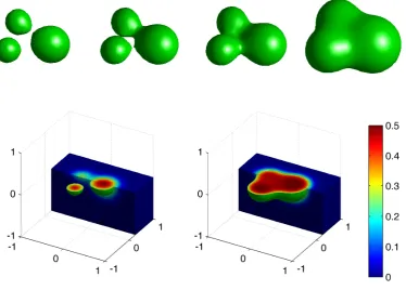
![Figure 2. Three-dimensional simulation of the Cahn-Hilliard equation on the computational domainΩ = [0, 1]3](https://thumb-us.123doks.com/thumbv2/123dok_us/8570074.368222/33.595.134.458.98.420/figure-dimensional-simulation-cahn-hilliard-equation-computational-domain.webp)