Enhancing the spatial resolution of satellite-derived land surface
temperature mapping for urban areas
Xiao Feng1∗, Giles Foody1, Paul Aplin1, Simon Gosling1
1 School of Geography, Sir Clive Granger Building, University of Nottingham, University Park, Nottingham, UK, NG7 2RD.
∗Corresponding author: Xiao Feng. Email: [email protected] Telephone: +00447985235817 Abstract: Land surface temperature (LST) is an important environmental variable for urban studies such as those focused on the urban heat island (UHI). Though satellite-derived LST could be a useful complement to traditional LST data sources, the spatial resolution of the thermal sensors limits the utility of remotely sensed thermal data. Here, a thermal sharpening technique is proposed which could enhance the spatial resolution of satellite-derived LST based on super-resolution mapping (SRM) and super-resolution reconstruction (SRR). This method overcomes the limitation of traditional thermal image sharpeners that require fine spatial resolution images for resolution enhancement. Furthermore, environmental studies such as UHI modelling typically use statistical methods which require the input variables to be independent, which means the input LST and other indices should be uncorrelated. The proposed Super-Resolution Thermal Sharpener (SRTS) does not rely on any surface index, ensuring the independence of the derived LST to be as independent as possible from the other variables that UHI modelling often requires. To validate the SRTS, its performance is compared against that of four popular thermal sharpeners: the thermal sharpening algorithm (TsHARP), adjusted stratified stepwise regression method (Stepwise), pixel block intensity modulation (PBIM), and emissivity modulation (EM). The privilege of using the combination of SRR and SRM was also verified by comparing the accuracy of SRTS with sharpening process only based on SRM or SRR. The results show that the SRTS can enhance the spatial resolution of LST with a magnitude of accuracy that is equal or even superior to other thermal sharpeners, even without requiring fine spatial resolution input. This shows the potential of SRTS for application in conditions where only limited meteorological data sources are available yet where fine spatial resolution LST is desirable.
Keywords: thermal sharpening, urban remote sensing, urban heat island, super-resolution mapping, super-resolution reconstruction.
1. Introduction
The majority of the global population resides in urban areas and the urban population is expected to further increase to more than 3 billion people by 2050 (Buhaug & Urdal, 2013). Cities are a focal point for economic and social activities and, therefore, are closely related to human daily life (Madlener & Sunak, 2011; Mirzaei & Haghighat, 2010). Attention is increasingly being given to the pursuit of more comfortable living conditions in urban areas in the face of increasing urbanisation. There is, therefore, growing interests in the factors that impact on human comfort and well-being in cities (Gago, Roldan, Pacheco-Torres, & Ordóñez, 2013; Kleerekoper, Van Esch, & Salcedo, 2012; Oke, 1982; Quattrochi & Luvall, 1999; Santamouris, 2013).
Many researchers have shown that the temperature of an urban area is generally higher than that of its surroundings (Gago, et al., 2013; Mirzaei & Haghighat, 2010). This phenomenon is known as the urban heat island (UHI) and this can be detrimental to human comfort. For instance, UHIs are often linked to poor air quality (Sarrat, Lemonsu, Masson, & Guedalia, 2006), and they can increase the energy demand of cities (M. Kolokotroni, Ren, Davies, & Mavrogianni, 2012; Maria Kolokotroni, Zhang, & Watkins, 2007; Kondo & Kikegawa, 2003; Mirzaei & Haghighat, 2010; Santamouris et al., 2001). UHIs can even contribute to human mortality rates, with thousands of heat-related deaths in cities every year (Ashley, Lemay, & Lionel; Cleveland, 2007; Gosling, Lowe, McGregor, Pelling, & Malamud, 2009). For example, some 50,000 deaths were caused by the 2003 European heat wave (Mirzaei & Haghighat, 2010). The UHI has been directly linked to adverse impacts on human health, and human thermal comfort in urban areas is expected to decline with climate change (Cheung & Hart, 2014; Tan et al., 2010). A considerable body of literature reports approaches to relieve the effect of the UHI with some initiatives already in operation (Rosenzweig et al., 2006; Schmidt, 2006). However, causes of the UHI can vary from place to place and thus there is no general or global understanding of, or solution for
problems associated with, UHIs (Mirzaei & Haghighat, 2010). It is acknowledged that temperature is closely related to land cover and hence much research has focused on this aspect (Weng, 2009). Urban areas represent a highly complex surface type which makes urban surface temperatures highly variable, both temporally and spatially (Prata, Caselles, Coll, Sobrino, & Ottlé, 1995; Vauclin, Vieira, Bernard, & Hatfield, 1982). Constructing high spatial resolution maps of urban temperature is an important first step towards analysing the UHI and in working towards solutions for its negative consequence for humans.
Traditional approaches to collect temperature data for mapping purposes are based upon weather station records and mobile equipment such as thermometers or sensors mounted on vehicles (Borbora & Das, 2014). Such approaches suffer from several major limitations. The spatial resolution of weather station data is, for example, typically very coarse since stations tend to be distributed very sparsely. For example, there are only 34 weather stations which record daily or hourly temperature
throughout Greater London, an area of 1572 km2
(http://badc.nerc.ac.uk/googlemap/midas_googlemap.cgi). Moreover, the temporal coverage of these stations is inconsistent, which means not all of them can be used for any specific date. When it comes to smaller cities such as Nottingham, UK, which covers around 422 km2, there are only six weather stations recording daily or hourly temperature. Although mobile temperature sensors can address the spatial resolution limitation to some extent by providing more measurements across a city, this approach cannot give a fully synchronised view over the whole city (Weng, 2009), and is also limited in terms of temporal coverage and can be a very costly undertaking.
Because of the problems with traditional methods, interest in remote sensing data for estimating land surface temperature (LST) is increasing as this approach can acquire data across large areas rapidly and regularly and has a much higher spatial sample density than weather station data. However, effective UHI analysis requires detailed and accurate information on urban heat flux and energy dynamics, and the relatively coarse spatial resolution of most spaceborne remote sensing systems
may be inadequate for this purpose. For example, the spatial resolution of one of the most widely used thermal image data sources, the Moderate Resolution Imaging Spectroradiometer (MODIS), is 1 km for the thermal bands, and 500 m/250 m for the optical bands. The spatial resolution of other meteorological satellite sensors such as the Geostationary Operational Environmental Satellite (GOES) can be as coarse as 4 km/8 km for the thermal band and 1 km/4 km for the optical bands. It can be noticed that optical bands tend to have finer spatial resolutions than thermal bands because they operate at shorter, more energy-rich, wavelengths. While some visible and near infrared (NIR) satellite sensors can provide imagery with sub-meter resolution, currently the finest spatial resolution thermal spaceborne image data is 60 m, provided by the Enhanced Thematic Mapper Plus (ETM+) on board Landsat 7. Although the Landsat 8 was launched in 2013, its thermal sensor has a spatial resolution of only 100 m, even coarser than that of Landsat 7. This relatively coarse spatial resolution may be affected strongly by mixed pixels, whereby each pixel comprises a mixture of two or more land cover types, especially in complex and spatially heterogeneous urban areas. Consequently, any attempt to predict urban LST from spaceborne imagery may suffer from considerable inaccuracy. One solution to this problem may be to use imagery from airborne sensors since these can provide considerably finer spatial resolution data than satellite sensors, but such sources are costly and not routinely available. A more realistic and achievable solution may be offered by ‘thermal sharpening’ methodologies, whereby fine spatial resolution optical imagery is integrated with coarser resolution thermal imagery to create a finer resolution thermal image output (Dominguez, Kleissl, Luvall, & Rickman, 2011; Zhan et al., 2013). Some such approaches are well-established; the earliest thermal sharpening technique dates back to the 1980s when, for example, Tom, Carlotto, & Scholten (1985) demonstrated such analysis on Landsat TM thermal data.
Various thermal sharpening methods are now available for use, but the accuracy of different methods can vary considerably for different land surface types. Given the major role of vegetation in modulating urban temperatures, most thermal sharpening methods are based on the empirical relationship between LST and a vegetation index (e.g. the Normalised Difference Vegetation Index
(NDVI)). For instance, fine spatial resolution NDVI data derived from optical imagery may be combined with coarser spatial resolution thermal imagery to predict LST at the finer resolution (Essa, Verbeiren, Van der Kwast, Van de Voorde, & Batelaan, 2012). However, the relationship between LST and NDVI can be unreliable under certain conditions such as where study areas have little vegetation present or where atmospheric conditions have high water vapour content (Chen, Yan, Ren, & Li, 2010; H. Yang, Cong, Liu, & Lei, 2010). In addition, the surface indices derived from remote sensing data are widely used as predictor variables in urban studies (e.g. UHI). Theoretically, the predictors in an analytical model should be independent (Osborne & Waters, 2002). It might be difficult to achieve absolute independence. However, the predictors for modelling should at least be as independent as possible. If the LST is derived with the aid of a surface index, that index will have a high correlation with the sharpened LST and may no longer be suitable for use as a predictor in a model together with the sharpened LST. This reduces the range of appropriate predictors available for the modelling work, thus limiting analysis. Further significant limitations of most current thermal sharpening methods are their requirement for both coarse and fine spatial resolution data and that the target (sharpened) spatial resolution is determined by the fine resolution input. That is, while it is possible to sharpen the coarse resolution data to a target resolution between that of the coarse and fine spatial resolution data, it is impossible to sharpen the coarse resolution data to a target resolution which is finer than the available fine resolution data. Additionally, while some sensors do acquire both fine resolution optical imagery and coarse resolution thermal imagery simultaneously (e.g. Landsat ETM+), this is not always the case. Where land cover changes slowly the optical and thermal data may not need to be strictly simultaneous. In this case, the data from different satellite sensors may be used. However, if a very fine spatial resolution (≤30 m) is required, the optical data is generally costly. In this paper, a method is proposed to enhance the spatial resolution of satellite-derived LST maps that does not require a fine resolution input and does not rely on any surface indices to sharpen the LST. It is based on two image processing techniques which could be used to enhance image spatial resolution: super-resolution mapping (SRM) and super-resolution reconstruction (SRR). Previous studies on SRM have focused on
enhancing the spatial resolution of land cover maps obtained from remotely sensed imagery. In this paper, SRM is used to enhance the spatial resolution of image-derived emissivity maps, one of the variables required to estimate LST from remotely sensed data. SRR has been widely used to generate a fine spatial resolution image by using a set of coarse spatial resolution images. This approach seeks to use the sub-pixel shifts between all the scenes to accumulate more detailed spatial information on the imaged area. Here, SRR has been used to enhance the spatial resolution of both the thermal radiance derived from the original satellite sensor image and atmospheric profiles involved in LST estimation which can either be derived from satellite sensor data or from other sources. This is achieved without use of a vegetation index. Many urban studies do not require ‘absolute’ temperature of each pixel and instead simply need to show the spatial pattern of ‘relative’ temperature variation across the study area (Weng, 2009). In this paper, the new SRTS is assessed for extracting spatial patterns of LST relative to established thermal sharpening methods which typically require additional data (e.g. vegetation index or fine spatial resolution image).
2. Super-Resolution Thermal Sharpener (SRTS)
The new thermal sharpening approach, which exploits SRM and SRR procedures, is hereby referred to as the Super-Resolution Thermal Sharpener (SRTS). This method provides the novelty and benefit of enhancing LST spatial resolution, but it also offers considerable flexibility since it can be implemented using any of a range of standard methods to derive LST in the first place. For instance, standard single-band (Qin, Karnieli, & Berliner, 2001) or split-window algorithms (Qin, Zhang, & Karnieli, 2001) can be used to derive LST, while SRTS enhances the resolution of the derived LST product.
Broadly, there are three main categories of LST estimation methods with known emissivity for each pixel in an image: (i) single-band methods, (ii) split-window methods which require imagery with two thermal bands, and (iii) multi-band methods which involve three or more bands. Here, since this
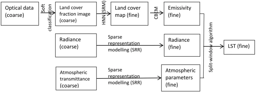
research uses MODIS data which has two thermal bands, a split-window method (Mao, Qin, Shi, & Gong, 2005) was used to estimate LST. This method has been shown to be relatively accurate and simple, requiring only three inputs: radiance, emissivity and atmospheric transmittance. All of these inputs are provided from the MODIS imagery. The SRTS operates essentially by enhancing the spatial resolution of the inputs to the split-window algorithm, thus rendering a fine spatial resolution LST data set. Initially, therefore, each of the three inputs must be processed independently before being combined to derive LST. The structure of the SRTS is shown in figure 1. After the fine spatial resolution inputs have been obtained from SRM and SRR algorithms, they are then input to the split-window algorithm and fine spatial resolution LST can be derived.
Fig 1. Workflow of the Super-Resolution Thermal Sharpener. CBEM represents the classification-based emissivity method and HNN means the Hopfield neural network.
2.1 Enhancing the spatial resolution of emissivity maps
It is known that emissivity is a crucial variable for LST estimation (Li, Tang, et al., 2013; Li, Wu, et al., 2013). The emissivity of a material is the ratio between the emittance of that material at temperature 𝑇𝑇 and the emittance of a blackbody at the same temperature. Many previous studies have used spectral indices such as NDVI to calculate emissivity, based on the assumption that NDVI is associated with emissivity. As mentioned above, if the surface index (e.g. NDVI) is used to sharpen the LST, the
Optical data (coarse) Land cover fraction image (coarse) Land cover map (fine) Radiance (fine) Atmospheric transmittance (coarse) Radiance
(coarse) LST (fine)
derived LST may have high correlation with the surface index used, limiting the value of the index for use in a later analysis of the fine resolution LST image. To avoid this problem, emissivity is derived without using spectral indices. Instead, land cover is used as the variable that determines emissivity. This approach assumes that each land cover class has a constant and predictable emissivity. First, land cover classification is conducted on the optical remotely sensed image and then emissivity values (as determined originally from laboratory tests) are allocated to each pixel according to its land cover type. This approach is known as the Classification-Based Emissivity derivation Method (CBEM) (Snyder, Wan, Zhang, & Feng, 1998). SRM may be incorporated into this emissivity estimation method to enhance the spatial resolution of a land cover and so ultimately an emissivity map. Using soft classification as an input (Foody, 1996), SRM exploits the class composition information of each pixel to map land cover at a fine (sub-pixel) resolution often through some form of iterative spatial analysis (Muad & Foody, 2012; Tatem, Lewis, Atkinson, & Nixon, 2001b). The final product is a fine spatial resolution land cover map which allows the characterisation of emissivity at this fine resolution. The zoom factor which determines the degree of sharpening achieved (e.g. sharpening or zooming from input coarse 1 km resolution imagery to output fine 250 m resolution imagery has a zoom factor of 4) can be specified by users. Various algorithms have been proposed for SRM (Boucher & Kyriakidis, 2006; Boucher, Kyriakidis, & Cronkite-Ratcliff, 2008; Verhoeye & De Wulf, 2002), but the Hopfield Neural Network (HNN) has proved popular(Tatem, Lewis, Atkinson, & Nixon, 2001a; Tatem, et al., 2001b). Here, a HNN-based SRM technique was used (Tatem, et al., 2001a). The fine resolution land cover map produced by SRM is then used to produce a fine resolution emissivity map which is used subsequently to calculate a fine resolution LST image.
The basis of the HNN is detailed by Tatem et al. (2001b) but some salient issues are outlined here. The structure of the HNN is designed as a representation of the fine spatial resolution image. Each neuron represents a sub-pixel of the original coarse resolution image (a pixel of the fine resolution image). For each class, there is a layer in which the number of neurons is the same as the number of the
pixels of the original coarse resolution image. The HNN operates by minimising an energy function while maximising the spatial correlation of all the neurons (Muad, 2011).
2.2 Enhancing the spatial resolution of radiance and atmospheric parameters
Radiance can be estimated from the thermal band of a sensor through the offset and scale factor provided for the sensor, and atmospheric parameters can be obtained either from the satellite imagery or weather station data (Qin, Zhang, et al., 2001). In this study, both of these variables are first estimated at the image’s original (coarse) spatial resolution, and then the resolution is enhanced through SRR. Traditionally, SRR reconstructs a fine spatial resolution image based on a series of coarse spatial resolution images (Siu & Hung, 2012). Standard SRR methods exploit sub-pixel shifts between multiple coarse resolution images, extracting information on high frequency details by projecting all the coarse images to a sub-pixel grid. However, it is not always possible to obtain a series of images over a short period of time. Thus, where the phenomenon of interest varies rapidly, as with temperature, traditional SRR can be impractical. Instead, here, a learning-based SRR method which involves a sparse representation model was used since this has no requirement for multi-temporal imagery (Yang, Wright, Huang, & Ma, 2008; Zeyde, Elad, & Protter, 2012).
The sparse representation model uses a vector with very limited number of non-zero elements and a matrix to represent another vector. Image can be expressed as one vector and thus the sparse representation model is considered to be applicable for representing an image (Yang, et al., 2008). In the sparse representation field, the vector with a small number of non-zero elements is called as sparse vector, while the matrix is called a dictionary (Aharon, Elad, & Bruckstein, 2006).
The basis of image sharpening through sparse representation modelling is that the images at different spatial resolutions share the same sparse vector (Yang, Wright, Huang, & Ma, 2010). This is the case because the sparse vector actually represents the characteristics of the land surface covered by the
image, but the dictionary matrix is the description of the land surface by the image. Hence, images at different spatial resolutions providing different descriptions of the surface use different dictionary matrices.
Based on the above discovery about the shared sparse vector, the sparse representation modelling based SRR method was developed (Yang, et al., 2008, 2010). This involves the derivation of dictionaries for the fine and coarse spatial resolution images; training images are used for this purpose (Aharon, et al., 2006; Zeyde, et al., 2012). These two dictionaries can then be used directly with images which have the same statistical characteristics as the training images (Yang, et al., 2008). This means, if the input image is a satellite-derived thermal image, such as in this study, the training images should be the same type of images. Because the training procedure will generate a corresponding coarse spatial resolution image for each training image, the training procedure does not require fine resolution images. Instead, training images have no limitation on spatial resolution but just need to be the same data type as the input image (Yang, et al., 2008).
3. Research methods and materials
This section outlines the established thermal sharpening methods that were used as the comparisons to the SRTS as well as the study area and data sets employed.
3.1 Study area and data preparation
London was selected as the study area for its large area and complex composition. Attention focused on four major surface land cover types of varying emissivity: impervious area, vegetation, water and bare soil. The image data used was a MODIS image acquired on 26/05/2012 and a Landsat Thematic Mapper (TM) image acquired on 25/05/2011. These near-anniversary images were used because
concurrent MODIS and Landsat images were not available for analysis. The best temporal match within the same calendar year was several month apart, with images affected significantly by cloud. Therefore, anniversary images were felt most appropriate since they avoid any seasonal effects.
With the SRTS, MODIS optical bands 1 -7 with 500 m spatial resolution were used firstly to derive the soft classification results by linear spectral unmixing (Mather, 2004), and then to obtain an emissivity map through the CBEM; bands 2 and 19 with 1 km spatial resolution were used to derive atmospheric transmittance; and thermal bands (31 and 32) at 1km resolution were used to calculate radiance. For the other thermal sharpening methods, coarse (1 km) spatial resolution LST and the associated indices were estimated directly from the 1 km MODIS data. The corresponding fine resolution indices are extracted from Landsat TM imagery (30 m). The reference data used for correlation analysis with the various sharpened LST outputs is the LST product from Advanced Spaceborne Thermal Emission and Reflection Radiometer (ASTER) with a spatial resolution of 90 m. ASTER data was used since this sensor shares the same satellite platform as MODIS thus ensuring acquisition time and atmospheric conditions are identical for both analysis and reference imagery. The Ordnance Survey (OS) Street
View map created from OS and downloaded from Digimap
(http://digimap.edina.ac.uk/digimap/home) was used as another type of reference for examining the accuracy of spatial distribution of the LST.
The target fine spatial resolution of the resolution-enhanced LST by each method in this experiment was set as 50 m. As such the analysis has a zoom factor of 20 (since the original MODIS image has a resolution of 1 km), larger than previous studies that have typically not exceeded 10 (Agam, Kustas, Anderson, Li, & Colaizzi, 2008; Agam, Kustas, Anderson, Li, & Neale, 2007).If successful this method allows the acquisition of LST with both high temporal and spatial resolution by sharpening MODIS thermal imagery (which has a high temporal resolution) to a relatively high spatial resolution similar to Landsat ETM+ thermal imagery (which has a low temporal resolution). This would aid monitoring
applications. Therefore, all the fine resolution indices as well as the ASTER validation data were resampled to 50 m using the nearest neighbour resampling algorithm.
3.2 Implementation of the SRTS and sharpening processes based on SRM or SRR only
The SRTS, on the one hand, firstly soft classified the MODIS band 1-7 to derive a series of fractional images at 500 m resolution for each land cover class. Then the HNN based SRM method was conducted based on those fractional images and output a classification map at 50 m resolution. Thereafter, the CBEM was implemented for this resolution-enhanced classified map and the emissivity map at 50m resolution was produced.
On the other hand, the sparse representation modelling based SRR method that the SRTS adopted was conducted to the 1 km radiance and atmospheric transmittance derived from the MODIS data, and output the 50 m radiance and transmittance images. Finally, all the 50 m emissivity, radiance and transmittance were input to the split-window algorithm to generate a LST map with 50m spatial resolution.
Here, to see the contributions of the SRM and SRR to the SRTS separately, thermal sharpening process based on only SRM or SRR was also designed (hereafter referred as SRM-only and SRR-only). These two processes only use one of the SRM and SRR in the thermal sharpening process of the SRTS. This means only some of the inputs to split-window were sharpened to 50 m. The solution to the rest inputs is to resample them by nearest neighbourhood sampling to make their image dimension the same as the resolution-enhanced input to split-window algorithm.
3.3 Traditional thermal sharpening methods
The implementation of other chosen comparing thermal sharpening methods is introduced here. All of them require both coarse and fine spatial resolution inputs. The coarse input in this experiment is
the 1 km LST derived from the original MODIS data, while the fine resolution inputs are derived from the resampled 50 m Landsat TM data.
TsHARP, adjusted stratified stepwise regression method (Stepwise) and pixel block intensity method (PBIM), all make use of the relationship between LST and remote sensing indices, such as NDVI or normalised difference of built-up area index (NDBI), to enhance the spatial resolution of the coarse resolution LST image. The assumption underlying these methods is that the relationship between LST and the selected index is scale-invariant. This means the relationship constructed between the coarse resolution index and LST should be the same as that between a fine resolution index and LST (Agam, et al., 2007). Traditional TsHARP is only based on the relationship between the NDVI and LST (Kustas, Norman, Anderson, & French, 2003). Here, the work of Agam et al. (2007) is followed in which not only NDVI is used; also used are the relationship of the fractional vegetation cover (Fc) and simplified fractional vegetation cover (sFc) with LST. Also, different regression tools have been tested for TsHARP. Thus, in the later results section, four results are presented for TsHARP with different combination of index and regression tool, including the linear regression with NDVI, Fc and sFc, and the quadratic regression with NDVI.
PBIM uses a fine spatial resolution LST image to sharpen a coarse LST image. The input coarse and fine spatial resolution LST images, however, are not necessarily acquired on the same day, but simply need to be acquired in the same season or month (Nichol, 2009). Stepwise uses NDVI, NDBI, Modified Normalised Difference Water Index (MNDWI) and albedo as predictors to build a statistical relationship with LST through an approach called stepwise multiple parameters regression (Zhu, Guan, Millington, & Zhang, 2012).
Emissivity modulation (EM) enhances spatial resolution of LST by using a resolution-enhanced emissivity image during the LST estimation procedure from the original thermal image (Nichol, 2009). It uses a fine spatial resolution map of emissivity, which is derived from a classification of fine
resolution optical imagery covering the same area of the thermal data through the CBEM, to sharpen the coarse resolution LST (Snyder, et al., 1998).
3.4 Validation
There is no ‘standard’ accuracy for the validation of thermal sharpening methods, and thus the validation of the proposed SRTS was in the comparing form with other existing popular thermal sharpening methods which were introduced in section 3.3. The focus of the research was to derive an enhanced ‘spatial’ representation of LST, rather than to necessarily calculate ‘absolute’ LST measurements. This focus was necessary partly because of fundamental difficulties in determining fully accurate LST values from remotely sensed imagery; however it has been shown that the spatial pattern of LST is very useful in urban planning or UHI analysis (Weng, 2009). Therefore, validation was conducted by comparing the ‘shape’ of objects with distinctive temperature characteristics, rather than their actual ‘temperature’. To assess the accuracy of the SRTS comprehensively, the similarity of both the statistical properties of the imagery and the spatial distribution of LST between predicted and reference LST were tested in this study.
Two metrics were used for accuracy assessment: root mean square error (RMSE) of the boundary of the selected object (which will be hereafter referred as boundary RMSE) and correlation coefficient between the predicted fine spatial resolution LST and the reference fine resolution LST (ASTER LST). The accuracy of mapping the boundary of an object was expressed as the RMSE of distance between predicted and reference boundary. Here the calculation was based on the Euclidean distance from equally spaced points with 50 meters interval along the predicted boundary to the reference boundary. For this LST-distinctive objects with clear boundaries were required. Five water reservoirs and three vegetated parks were chosen as the LST-distinctive objects for calculation of boundary RMSE. These are all man-made objects and for the most comprise relatively straight or smooth boundaries
representing features that are easily detectable. However, the objects do also contain some irregular boundary features such as sharp corners and these represent features that are not easily detectable. The existence of both simple and complex boundary features ensure a comprehensive test of the ability of each method to characterise shape and location of LST. The boundaries of reservoirs and parks on both the vector map and the derived LST images were extracted manually. Because TsHARP, which is based on NDVI, is theoretically unavailable for water surface, only the boundary RMSE of parks was used for comparison between different methods including TsHARP results.
4. Results and discussion
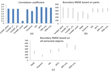
Analysis was conducted using the methods and data described in section 3, producing, in total, ten fine (50m) spatial resolution LST images derived by (a) TsHARP_NDVI, (b) TsHARP_Fc, (c) TsHARP_sFc, (d) TsHARP_quad, (e) Stepwise, (f) PBIM, (g) EM, (h) SRTS, (i) SRR-only, and (j) SRM-only. These were compared against the ASTER-derived reference LST map and, in each case, correlation coefficient between the sharpened LST and the ASTER LST was calculated (figure 2(a)). Also, average boundary RMSE with its standard error of the LST sharpened by different thermal sharpening methods were calculated based on different types of surface. Comparison of average boundary RMSE of parks between all methods was shown in figure 2(b), while boundary RMSE of all extracted objects was conducted on all methods except TsHARP (figure 2(c)).
Through the comprehensive comparison of different thermal sharpening methods by correlation analysis between the thermal sharpeners and the reference, and boundary RMSE of the objects extracted from the sharpened LSTs, it can be seen that the accuracy of the proposed SRTS is comparable with other thermal sharpening methods. Given that the SRTS does not rely on any fine resolution information while enhancing the spatial resolution of LST with a large zoom factor, this indicates the value of the technique. The overall comparison of correlation coefficients shows that the
SRTS obtained the second highest correlation with the reference, higher than most of the existing thermal methods, indicating the statistical nature of the SRTS sharpened LST is more similar to that of the reference LST than most other methods.
(a) (b)
Correlation coefficient Boundary RMSE based on parks
0 0.1 0.2 0.3 0.4 0.5 0.6 0.7 0.8 0 100 200 300 400 500 600 0 100 200 300 400 500 600
700 Boundary RMSE based on all extracted objects
[image:16.595.105.486.172.423.2](c)
Fig 2. Evaluation of thermal sharpening results. (a) Whole image correlation with reference data for ten different thermal sharpening methods (b) Average boundary RMSE plus/minus 1x standard error of exacted parks from LST sharpened by each method. (c) Average boundary RMSE plus/minus 1x standard error of all the extracted objects from LST sharpened by all the methods except TsHARP. TsHARP_NDVI = TsHARP method using linear regression and NDVI, TsHARP_Fc = TsHARP method using linear regression and Fc, TsHARP_sFc = TsHARP method using linear regression and sFc, TsHARP_quad = TsHARP method using quadratic regression and NDVI, Stepwise = adjusted stratified stepwise regression method, PBIM = pixel block intensity modulation, EM = emissivity modulation, SRTS = super-resolution thermal sharpener, SRR-only = thermal sharpening procedure of SRTS only using SRR sharpened product, SRM-only = thermal sharpening procedure of SRTS only using SRM sharpened product.
Through the average RMSE with its standard error of parks (figure 2(b)), it can be seen that, except Stepwise which obtained a significantly small RMSE, the ability of SRTS on detecting boundary is similar to those of all other methods because their RMSEs do not significantly different from RMSE of the SRTS. Although the boundary RMSEs of parks of both EM and SRTS seem to be higher than that of PBIM (figure 2(b)), which may suggest that they are not good at detecting clear boundary for
vegetation, the boundary RMSE of all extracted objects (figure 2(c)) shows that the RMSEs of EM, SRTS and PBIM are generally similar when other type of surfaces were considered.
All the above figures indicate that though the SRTS may be as good as Stepwise, it has the similar accuracy of detecting boundary with most other methods. Moreover, this accuracy is achieved by SRTS without any fine spatial resolution information during sharpening and this is the most important priority of the proposed SRTS, as it could be implemented to any conditions no matter whether the fine spatial resolution data is available.
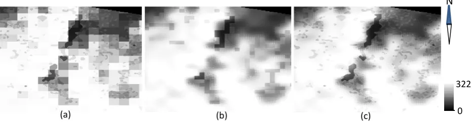
[image:17.595.77.543.503.624.2]In comparison of SRTS, SRR-only and SRM-only methods through correlation coefficient (figure 2(a)) and boundary RMSE of all extracted objects (figure 2(c)), it can be seen that the correlation between the sharpened LST and the reference LST was enhanced largely by the combining usage of SRM and SRR. The boundary RMSE of objects extracted from the LST sharpened by SRTS was also enhanced to some extent. This might be because the blocky nature of the SRM-only result was balanced by introducing the SRR to sharpen the radiance and atmospheric transmittance (figure 3(a)), while the boundary definition in SRR result was enhanced by incorporating the SRM-processed emissivity (figure 3(b)).
Fig 3 Comparison of the LST derived by SRM-only method (a), SRR-only method (b) and SRTS (c). These are three lakes in the study area where the surrounding area of the lakes are vegetation and impervious surfaces. The spatial resolution for each image is 50 m.
The boundary RMSE is only based on some extracted objects, using for reflecting the ability of methods on detecting exact boundary of objects. It could indicate the shape and locational accuracies of the spatial distribution of LST from certain aspects. Nevertheless, the visual comparison of the
N
0 322
(a) (b) (c)
entire LST image derived from all the methods may be able to provide a more straight forward and comprehensive way to illustrate their ability on extracting spatial pattern of LST.
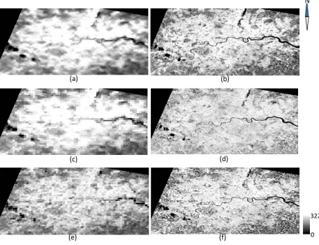
The sharpened LST images obtained from the SRTS, Stepwise, EM, PBIM and TsHARP with NDVI were illustrated in figure 4 as well as the ASTER LST which was used as the reference data. It can be seen that the spatial pattern of the SRTS sharpened LST is generally consistent with the ASTER LST. Noticeably, this LST is sharpened without any fine spatial resolution information which is what all other methods required for sharpening. The visual interpretation of the LST images derived by different methods over the entire study area supports the conclusion that the accuracy of the SRTS is competitive with other existing thermal sharpeners.
In total, the results show that SRTS is broadly comparable with the traditional thermal sharpening methods. However, it is particularly important to recognise here that the SRTS uses only coarse spatial resolution data to calculate LST, while the other, pre-existing methods all require fine spatial resolution imagery as an input to identify LST-related factors such as vegetation. Thus, when the imagery with the desired fine spatial resolution is not available or very costly for analysis, the SRTS holds a major advantage over other thermal sharpening approaches, still enabling relatively high LST mapping accuracy.
More importantly, the SRTS is not especially proposed for MODIS. Actually SRTS is a method frame in which the structure can be altered according to different LST estimation method. For example, this experiment use split-window algorithm proposed by Qin et al. (2001b)which require radiance, emissivity and atmospheric transmittance as inputs. Thus the SRR was conducted to radiance and transmittance while SRM was conducted to emissivity. However, if SRTS is used to Landsat TM thermal data by using a single-window algorithm (Qin, et al., 2001a), the processing data for SRR will only be the radiance, while the SRM will still be implemented for emissivity. Therefore, the SRTS can be used for a wide range of data type and does not require the fine spatial resolution data for sharpening. This provide the urban-related studies the possibility to derive a fine or very fine spatial
resolution LST from a coarse or medium resolution data without requirement of additional fine resolution input.
(a) (b)
(c) (d)
(e) (f)
[image:19.595.77.535.125.476.2]
Fig 4 The sharpened LST images obtained from the different thermal sharpening methods for the entire study area (Great London), of which are (a) SRTS sharpened LST, (b) ASTER LST, (c) EM sharpened LST, (d) Stepwise sharpened LST, (e) TsHARP sharpened LST with NDVI, and (f) PBIM sharpened LST.
5. Conclusion
This paper introduced a new thermal sharpening approach for urban area: the Super-Resolution Thermal Sharpener (SRTS). Results show that the SRTS can enhance the spatial resolution of LST and achieve an accuracy that is comparable with existing thermal sharpening approaches. Importantly, however, the SRTS uses only coarse resolution data input while the other methods require fine spatial resolution data. Thus the SRTS holds considerable advantage over other thermal sharpeners and offers much greater flexibility for application where data sources are limited. In addition, the
N
0 322
zoom factor is no longer dictated by the fine resolution input but is set by users themselves. A further strength and novelty of the proposed method is that the enhanced resolution LST is derived independent from land cover related indices such as the NDVI, NDBI, or albedo, which may facilitate later environmental analyses, such as UHI, which use the fine resolution LST image derived. Further research will focus on addressing improving the locational accuracy of the boundary as well as seeking to improve boundary smoothness by enhancing the accuracy of SRM. Nevertheless, the significant potential of the proposed SRTS for enhancing the spatial resolution of LST when no corresponding fine resolution data is available has been demonstrated. Importantly, the method provides a convenient technique for application in future studies of urban climate, which require information on spatial patterns of LST at both frequent temporal and fine spatial resolutions.
Acknowledgements
We would like to thank Dr. Anuar Muad who provided the HNN Matlab code and guidance on its use. Also, many thanks to Yang J.C. who made the sparse representation model based SRR Matlab code available online free of charge.
References
Agam, N., Kustas, W. P., Anderson, M. C., Li, F., & Colaizzi, P. D. (2008). Utility of thermal image sharpening for monitoring field-scale evapotranspiration over rainfed and irrigated agricultural regions. Geophysical Research Letters, 35(2), L02402.
Agam, N., Kustas, W. P., Anderson, M. C., Li, F. Q., & Neale, C. M. U. (2007). A vegetation index based technique for spatial sharpening of thermal imagery. Remote Sensing of Environment, 107(4), 545-558.
Aharon, M., Elad, M., & Bruckstein, A. (2006). K -SVD: An Algorithm for Designing Overcomplete Dictionaries for Sparse Representation. Signal Processing, IEEE Transactions on, 54(11), 4311-4322.
Ashley, E., Lemay, & Lionel. Concrete’s contribution to sustainable development, from
http://www.specifyconcrete.org/assets/docs/Concretes_%20Contribution_to_Sustainable_ Development.pdf
Borbora, J., & Das, A. K. (2014). Summertime Urban Heat Island study for Guwahati City, India.
Sustainable Cities and Society, 11(0), 61-66.
Boucher, A., & Kyriakidis, P. C. (2006). Super-resolution land cover mapping with indicator geostatistics.
Remote Sensing of Environment, 104(3), 264-282.
Boucher, A., Kyriakidis, P. C., & Cronkite-Ratcliff, C. (2008). Geostatistical solutions for super-resolution land cover mapping. Ieee Transactions on Geoscience and Remote Sensing, 46(1), 272-283. Buhaug, H., & Urdal, H. (2013). An urbanization bomb? Population growth and social disorder in cities.
Global Environmental Change, 23(1), 1-10.
Chen, L., Yan, G., Ren, H., & Li, A. (2010, 25-30 July 2010). A modified vegetation index based algorithm
for thermal imagery sharpening. Paper presented at the Geoscience and Remote Sensing
Symposium (IGARSS), 2010 IEEE International.
Cheung, C., & Hart, M. (2014). Climate change and thermal comfort in Hong Kong. International
Journal of Biometeorology, 58(2), 137-148.
Cleveland, C. (2007). Heat Island Encyclopedia of Earth.
Dominguez, A., Kleissl, J., Luvall, J. C., & Rickman, D. L. (2011). High-resolution urban thermal sharpener (HUTS). Remote Sensing of Environment, 115(7), 1772-1780.
Essa, W., Verbeiren, B., Van der Kwast, J., Van de Voorde, T., & Batelaan, O. (2012). Evaluation of the DisTrad thermal sharpening methodology for urban areas. International Journal of Applied
Earth Observation and Geoinformation, 19, 163-172.
Foody, G. M. (1996). Approaches for the production and evaluation of fuzzy land cover classifications from remotely-sensed data. International Journal of Remote Sensing, 17(7), 1317-1340. Gago, E. J., Roldan, J., Pacheco-Torres, R., & Ordóñez, J. (2013). The city and urban heat islands: A
review of strategies to mitigate adverse effects. Renewable and Sustainable Energy Reviews, 25(0), 749-758.
Gosling, S., Lowe, J., McGregor, G., Pelling, M., & Malamud, B. (2009). Associations between elevated atmospheric temperature and human mortality: a critical review of the literature. Climatic
Change, 92(3-4), 299-341.
Kleerekoper, L., Van Esch, M., & Salcedo, T. B. (2012). How to make a city climate-proof, addressing the urban heat island effect. Resources, Conservation and Recycling, 64(0), 30-38.
Kolokotroni, M., Ren, X., Davies, M., & Mavrogianni, A. (2012). London's urban heat island: Impact on current and future energy consumption in office buildings. Energy and Buildings, 47(0), 302-311.
Kolokotroni, M., Zhang, Y., & Watkins, R. (2007). The London Heat Island and building cooling design.
Solar Energy, 81(1), 102-110.
Kondo, H., & Kikegawa, Y. (2003). Temperature Variation in the Urban Canopy with Anthropogenic Energy Use. pure and applied geophysics, 160(1-2), 317-324.
Kustas, W. P., Norman, J. M., Anderson, M. C., & French, A. N. (2003). Estimating subpixel surface temperatures and energy fluxes from the vegetation index-radiometric temperature relationship. Remote Sensing of Environment, 85(4), 429-440.
Li, Z. L., Tang, B. H., Wu, H., Ren, H. Z., Yan, G. J., Wan, Z. M., . . . Sobrino, J. A. (2013). Satellite-derived land surface temperature: Current status and perspectives. Remote Sensing of Environment, 131, 14-37.
Li, Z. L., Wu, H., Wang, N., Qiu, S., Sobrino, J. A., Wan, Z. M., . . . Yan, G. J. (2013). Land surface emissivity retrieval from satellite data. International Journal of Remote Sensing, 34(9-10), 3084-3127. Madlener, R., & Sunak, Y. (2011). Impacts of urbanization on urban structures and energy demand:
What can we learn for urban energy planning and urbanization management? Sustainable
Cities and Society, 1(1), 45-53.
Mao, K., Qin, Z., Shi, J., & Gong, P. (2005). A practical split‐window algorithm for retrieving land‐ surface temperature from MODIS data. International Journal of Remote Sensing, 26(15), 3181-3204.
Mather, P. M. (2004). Computer Processing of Remotely-Sensed Images: An Introduction, 3th Edition. Chichester, West Sussex, England: John Wiley & Sons Ltd.
Mirzaei, P. A., & Haghighat, F. (2010). Approaches to study Urban Heat Island – Abilities and limitations.
Building and Environment, 45(10), 2192-2201.
Muad, A. M. (2011). Super resolution mapping. PhD, University of Nottingham, Nottingham.
Muad, A. M., & Foody, G. M. (2012). Super-resolution mapping of lakes from imagery with a coarse spatial and fine temporal resolution. International Journal of Applied Earth Observation and
Geoinformation, 15, 79-91.
Nichol, J. (2009). An Emissivity Modulation Method for Spatial Enhancement of Thermal Satellite Images in Urban Heat Island Analysis. Photogrammetric Engineering & Remote Sensing, 75(5), 547-556.
Oke, T. R. (1982). The Energetic Basis of the Urban Heat-Island. Quarterly Journal of the Royal
Meteorological Society, 108(455), 1-24.
Osborne, J., & Waters, E. (2002). Four assumptions of multiple regression that researchers should always test. Practical assessment, research & evaluation, 8(2), 9.
Prata, A. J., Caselles, V., Coll, C., Sobrino, J. A., & Ottlé, C. (1995). Thermal remote sensing of land surface temperature from satellites: Current status and future prospects. Remote Sensing
Reviews, 12(3-4), 175-224.
Qin, Z., Karnieli, A., & Berliner, P. (2001). A mono-window algorithm for retrieving land surface temperature from Landsat TM data and its application to the Israel-Egypt border region.
International Journal of Remote Sensing, 22(18), 3719-3746.
Qin, Z., Zhang, M., & Karnieli, A. (2001). Split window algorithms for retrieving land surface temperature from NOAA-AVHRR data. Remote sensing for Land and Resources, 48(2), 10. Quattrochi, D. A., & Luvall, J. C. (1999). Thermal infrared remote sensing for analysis of landscape
ecological processes: methods and applications. Landscape Ecology, 14(6), 577-598.
Rosenzweig, C., Solecki, W., Parshall, L., Gaffin, S., Lynn, B., Goldberg, R., . . . Hodges, S. (2006). Mitigating New York City's Heat Island with Urban Forestry, Living Roofs, and Light Surfaces. Paper presented at the The 86th AMS Annual Meeting, Atlanta, GA.
Santamouris, M. (2013). Using cool pavements as a mitigation strategy to fight urban heat island—A review of the actual developments. Renewable and Sustainable Energy Reviews, 26(0), 224-240.
Santamouris, M., Papanikolaou, N., Livada, I., Koronakis, I., Georgakis, C., Argiriou, A., & Assimakopoulos, D. N. (2001). On the impact of urban climate on the energy consumption of buildings. Solar Energy, 70(3), 201-216.
Sarrat, C., Lemonsu, A., Masson, V., & Guedalia, D. (2006). Impact of urban heat island on regional atmospheric pollution. Atmospheric Environment, 40(10), 1743-1758.
Schmidt, M. (2006). The contribution of rainwater harvesting against global warming Berlin, Germany: Technische Universität Berlin.
Siu, W.-C., & Hung, K.-W. (2012, 3-6 Dec. 2012). Review of image interpolation and super-resolution. Paper presented at the Signal & Information Processing Association Annual Summit and Conference (APSIPA ASC), 2012 Asia-Pacific.
Snyder, W. C., Wan, Z., Zhang, Y., & Feng, Y. Z. (1998). Classification-based emissivity for land surface temperature measurement from space. International Journal of Remote Sensing, 19(14), 2753-2774.
Tan, J., Zheng, Y., Tang, X., Guo, C., Li, L., Song, G., . . . Chen, H. (2010). The urban heat island and its impact on heat waves and human health in Shanghai. International Journal of Biometeorology, 54(1), 75-84.
Tatem, A. J., Lewis, H. G., Atkinson, P. M., & Nixon, M. S. (2001a). Multiple-class land-cover mapping at the sub-pixel scale using a Hopfield neural network. International Journal of Applied Earth
Observation and Geoinformation, 3(2), 184-190.
Tatem, A. J., Lewis, H. G., Atkinson, P. M., & Nixon, M. S. (2001b). Super-resolution target identification from remotely sensed images using a Hopfield neural network. Ieee Transactions on
Geoscience and Remote Sensing, 39(4), 781-796.
Vauclin, M., Vieira, S. R., Bernard, R., & Hatfield, J. L. (1982). Spatial variability of surface temperature along two transects of a bare soil. Water Resources Research, 18(6), 1677-1686.
Verhoeye, J., & De Wulf, R. (2002). Land cover mapping at sub-pixel scales using linear optimization techniques. Remote Sensing of Environment, 79(1), 96-104.
Weng, Q. H. (2009). Thermal infrared remote sensing for urban climate and environmental studies: Methods, applications, and trends. Isprs Journal of Photogrammetry and Remote Sensing, 64(4), 335-344.
Yang, H., Cong, Z., Liu, Z., & Lei, Z. (2010). Estimating sub-pixel temperatures using the triangle algorithm. International Journal of Remote Sensing, 31(23), 6047-6060.
Yang, J., Wright, J., Huang, T., & Ma, Y. (2008, 23-28 June 2008). Image super-resolution as sparse
representation of raw image patches. Paper presented at the Computer Vision and Pattern
Recognition, 2008. CVPR 2008. IEEE Conference on.
Yang, J., Wright, J., Huang, T., & Ma, Y. (2010). Image Super-Resolution Via Sparse Representation.
Ieee Transactions on Image Processing, 19(11), 2861-2873.
Zeyde, R., Elad, M., & Protter, M. (2012). On Single Image Scale-Up Using Sparse-Representations. In J.-D. Boissonnat, P. Chenin, A. Cohen, C. Gout, T. Lyche, M.-L. Mazure & L. Schumaker (Eds.),
Curves and Surfaces (Vol. 6920, pp. 711-730): Springer Berlin Heidelberg.
Zhan, W. F., Chen, Y. H., Zhou, J., Wang, J. F., Liu, W. Y., Voogt, J., . . . Li, J. (2013). Disaggregation of remotely sensed land surface temperature: Literature survey, taxonomy, issues, and caveats.
Remote Sensing of Environment, 131, 119-139.
Zhu, S., Guan, H., Millington, A. C., & Zhang, G. (2012). Disaggregation of land surface temperature over a heterogeneous urban and surrounding suburban area: a case study in Shanghai, China.
International Journal of Remote Sensing, 34(5), 1707-1723.