Hierarchical Bayesian level set inversion

Noname manuscript No. (will be inserted by the editor)

Hierarchical Bayesian Level Set Inversion

Matthew M. Dunlop · Marco A. Iglesias · Andrew M. Stuart

Received: date / Accepted: date

Abstract The level set approach has proven widely successful in the study of inverse problems for inter-faces, since its systematic development in the 1990s. Re-cently it has been employed in the context of Bayesian inversion, allowing for the quantification of uncertainty within the reconstruction of interfaces. However the Bayesian approach is very sensitive to the length and amplitude scales in the prior probabilistic model. This paper demonstrates how the scale-sensitivity can be cir-cumvented by means of a hierarchical approach, using a single scalar parameter. Together with careful con-sideration of the development of algorithms which en-code probability measure equivalences as the hierar-chical parameter is varied, this leads to well-defined Gibbs based MCMC methods found by alternating Metropolis-Hastings updates of the level set function and the hierarchical parameter. These methods demon-strably outperform non-hierarchical Bayesian level set methods.

Keywords Inverse problems for interfaces_·Level set inversion_·Hierarchical Bayesian methods

1 Introduction 1.1 Background

The level set method has been pervasive as a tool for the study of interface problems since its introduction in Matthew M. Dunlop·Andrew M. Stuart

Computing & Mathematical Sciences, California Institute of Technology, Pasadena, CA 91125, USA

Marco A. Iglesias

School of Mathematical Sciences, University of Nottingham, Nottingham, NG7 2RD, UK

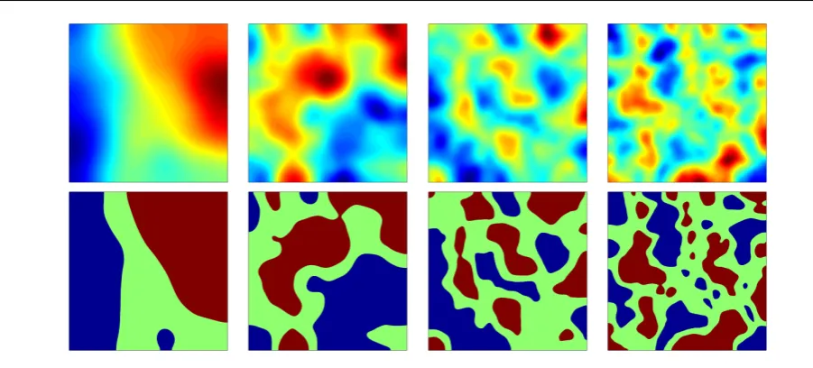
the 1980s [43]. In a seminal paper in the 1990s, Santosa demonstrated the power of the approach for the study of inverse problems with unknown interfaces [47]. The key benefit of adopting the level set parametrization of interfaces is that topological changes are permitted. In particular for inverse problems the number of connected components of the field does not need to be known a priori. The idea is illustrated in Figure 1. The type of unknown functions that we might wish to reconstruct are piecewise continuous functions, illustrated in the bottom row by piecewise constant ternary functions. However in the inversion we work with a smooth func-tion, shown in the top row and known as the level-set function, which is thresholded to create the desired unknown function in the bottom row. This allows the inversion to be performed on smooth functions, and allows for topological changes to be detected during the course of algorithms. After Santosa’s paper there were many subsequent papers employing the level set representation for classical inversion, and examples in-clude [11, 15, 19, 52], and the references therein.

constant permeabilities/conductivities in groundwater flow/electrical impedance tomography (EIT) models.

For linear Bayesian inverse problems, the adoption of Gaussian priors leads to Gaussian posteriors, formu-lae for which can be explicitly computed [22, 37, 41]. However thelevel set map, which takes the smooth un-derlying level set function (top row, Figure 1) into the physical unknown function (bottom row, Figure 1) is nonlinear; indeed it is discontinuous. As a consequence, Bayesian level set inversion, even for inverse problems which are classically-speaking ‘linear’, does not typi-cally admit closed form solutions for the posterior dis-tribution on the level set function. Thus, in order to pro-duce samples from the posterior arising in the Bayesian approach, MCMC methods are often used. Since the posterior is typically defined on an infinite-dimensional space in the context of inverse problems, it is important that the MCMC algorithms used are well-defined on such spaces. A formulation of the Metropolis-Hastings algorithm on general state spaces is given in [53]. A par-ticular case of this algorithm, well-suited to posterior distributions on function spaces and Gaussian priors, is the preconditioned Crank-Nicolson (pCN) method in-troduced (although not named this way) in [7]. As the method is defined directly on a function space, it has desirable properties related to discretization – in par-ticular the method is robust with respect to mesh re-finement (discretization invariance) – see [16] and the references therein. On the other hand, the need for hier-archical models in Bayesian statistics, and in particular in the context of non-parametric (i.e. function space) methods in machine learning, is well-established [8]. However, care is needed when using hierarchical meth-ods in order to ensure that discretization invariance is not lost [3]. In this paper we demonstrate how hier-archical methods can be employed in the context of discretization-invariant MCMC methods for Bayesian level set inversion.

1.2 Key Contributions of the Paper

The key contribution of this paper is in computational statistics: we develop a Metropolis Hastings method with mesh-independent mixing properties that makes an order of magnitude of improvement in the Bayesian level set method as introduced in [31].

Study of Figure 1 suggests that the ability of the level set representation to accurately reconstruct piece-wise continuous fields depends on two important scale parameters:

– the length-scale of the level set function, and its relation to the typical separation between disconti-nuities;

– the amplitude-scale of the level set function, and its relation to the levels used for thresholding.

If these two scale parameters are not set correctly then MCMC methods to determine the level set func-tion from data can perform poorly. This immediately suggests the idea of using hierarchical Bayesian meth-ods in which these parameters are learned from the data. However there is a second consideration which in-teracts with this discussion. From the work of Tierney [53] it is known that absolute continuity of certain mea-sures arising in the definition of Metropolis-Hastings methods is central to their well-definedness, and hence to discretization invariant MCMC methods [16]. In fact it appears algorithms defined on infinite dimensional spaces have spectral gaps that are bounded indepen-dently of the mesh, and so their convergence rates are bounded below in the limit [26]. The key contribution of our paper is to show how enforcing absolute continuity links the two scale parameters, and hence leads to the construction of a hierarchical Bayesian level set method with asingle scalarhierarchical parameter which deals with the scale and absolute continuity issues simulta-neously, resulting in e↵ective sampling algorithms.

The hierarchical parameter is an inverse length-scale within a Gaussian random field prior for the level set function. In order to preserve absolute continuity of dif-ferent priors on the level set function as the length-scale parameter varies, and relatedly to make well-defined MCMC methods, the mean square amplitude of this Gaussian random field must decay proportionally to a power of the inverse length-scale. It is thus natural that the level values used for thresholding should obey this power law relationship with respect to the hierarchical parameter. As a consequence the likelihood depends on the hierarchical parameter, leading to a novel form of posterior distribution.

groundwa-Fig. 1 Four continuous scalar fields (top) and the corresponding ternary fields formed by thresholding these fields at two levels (bottom). The smooth function in the top row is known as thelevel-set functionand is used in the inversion procedure. The discontinuous function in the bottom row is the physical unknown.

ter flow (in which measurements are made in the inte-rior of the domain) and EIT (in which measurements are made on the boundary).

1.3 Structure of the Paper

In section 2 we describe a family of prior distributions on the level set function, indexed by an inverse length scale parameter, which remain absolutely continuous with respect to one another when we vary this parame-ter; we then place a hyper-prior on this parameter. We describe an appropriate level set map, dependent on the length-scale parameter because length and ampli-tude scales are intimately connected through absolute continuity of measures, to transform these fields into piecewise constant ones, and use this level set map in the construction of the likelihood. We end by showing existence and well-posedness of the posterior distribu-tion on the level set funcdistribu-tion and the inverse length scale parameter. In section 3 we describe a Metropolis-within-Gibbs MCMC algorithm for sampling the poste-rior distribution, taking advantage of existing state-of-the-art function space MCMC, and the absolute conti-nuity of our prior distributions with respect to changes in the inverse length scale parameter, established in the previous section. Section 4 contains numerical experi-ments for three di↵erent forward models: a linear map comprising pointwise observations, groundwater flow and EIT; these illustrate the behavior of the algorithm and, in particular, demonstrate significant improvement

with respect to non-hierarchical Bayesian level set in-version.

2 Construction of the Posterior

In subsection 2.1 we recall the definition of the Whittle-Mat´ern covariance functions, and define a related fam-ily of covariances parametrized by an inverse length scale parameter ⌧. We use these covariances to define our prior on the level set functionu, and also place a hyperprior on the parameter⌧, yielding a priorP(u,⌧) on a product space. In subsection 2.2 we construct the level set map, taking into account the amplitude scal-ing of prior samples with ⌧, and incorporate this into the forward map. The inverse problem is formulated, and the resulting likelihoodP(y_|u,⌧) is defined. Finally in subsection 2.3 we construct the posterior P(u,⌧|y) by combining the prior_P(u,⌧) and likelihood_P(y_|u,⌧) using Bayes’ formula. Well-posedness of this posterior is established.

2.1 Prior

demonstrated in [20, 31]. A family of covariances pa-rameterized by length scale is hence required.

A widely used family of distributions, allowing for control over sample regularity, amplitude and length scale, are Whittle-Mat´ern distributions. These are a family of stationary Gaussian distributions with covari-ance function

c ,⌫,`(x, y) = 2 21 ⌫

(⌫) ✓

|x y|

`

◆⌫ K⌫

✓ |x y|

`

◆

where K⌫ is the modified Bessel function of the sec-ond kind of order⌫ [42, 50]. These covariances interpo-late between exponential covariance, for ⌫ = 1/2, and Gaussian covariance, for ⌫ _{! 1}. As a consequence, the regularity of samples increases as the parameter ⌫

increases. The parameter ` > 0 acts as a characteris-tic length scale (sometimes referred to as the spatial range) and as an amplitude scale ( 2 <sub>is sometimes</sub> referred to as the marginal variance). On <sub>R</sub>d<sub>, samples</sub> from a Gaussian distribution with covariance function c ,⌫,`correspond to the solution of a particular stochas-tic partial di↵erential equation (SPDE). This SPDE can be derived using the Fourier transform and the spectral representation of covariance functions – the paper [36] derives the appropriate SPDE for the covariance func-tion above:

1 p

`d(I ` 2

4)(⌫+d/2)/2v=W (1)

whereW is a white noise on_Rd_{, and}

= 22

d_⇡d/2 _(⌫+d/2)

(⌫) .

Computationally, implementation of this SPDE ap-proach requires restriction to a bounded subset D _✓

Rd_{, and hence the provision of boundary conditions} for the SPDE in order to obtain a unique solution. Choice of these boundary conditions may significantly a↵ect the autocorrelations near the boundary. The ef-fects for di↵erent boundary conditions are discussed in [36]. Nonetheless, the computational expediency of the SPDE formulation makes the approach very attrac-tive for applications and, if necessary, boundary e↵ects can be ameliorated by generating the random fields on larger domains which are a superset of the domain of interest.

From (1) it can be seen that the covariance operator corresponding to the covariance functionc ,⌫,` is given by

D ,⌫,`= `d(I `24) ⌫ d/2. (2) The fact that the scalar multiplier in front of the co-variance operator <sub>D</sub> ,⌫,` changes with the length-scale

means that the family of measures_{N(0,_D ,⌫,`)}`, for fixed and⌫, are mutually singular. This leads to prob-lems when trying to design hierarchical methods based around these priors. We hence work instead with the modified covariances

C↵,⌧ = (⌧2I 4) ↵

where ⌧ = 1/` > 0 now represents an inverse length scale, and ↵=⌫+d/2 still controls the sample regu-larity. To be concrete we will always assume that the domain of the Laplacian is chosen so that_C↵,⌧ is well-defined for all⌧ 0; for example we may choose a pe-riodic box, with domain restricted to functions which integrate to zero over the box, Neumann boundary con-ditions on a box, again with domain restricted to func-tions which integrate to zero over the box, or Dirichlet boundary conditions. We have the following theorem concerning the family of Gaussians {N(0,C↵,⌧)}⌧ 0, proved in the Appendix.

Theorem 1 Let D = _Td _{be the d-dimensional torus,}

and fix ↵>0. Define the family of Gaussian measures

µ⌧

0=N(0,C↵,⌧),⌧ 0. Then

(i) ford3, the{µ⌧

0}⌧ 0 are mutually equivalent; (ii) if u_⇠µ⌧

0, then µ⌧0-a.s. we have u2 Hs(D) and u₂Cbsc,s bsc_{(D)for all s <↵ d/2.} 1

(iii) ifu⇠µ⌧

0 andv⇠N(0,D ,⌫,`), then

Eku_k2

/⌧d 2↵ ·Ekv_k2

with constant of proportionality independent of⌧.

Remark 1 (a) Proof of this theorem is driven by the smoothness of the eigenfunctions of the Lapla-cian subject to periodic boundary conditions, to-gether with the growth of the eigenvalues, which is like j2/d_{.These properties extend to Laplacians} on more general domains and with more general boundary conditions, and to Laplacians with lower order perturbations, and so the above result still holds in these cases. For discussion of this in rela-tion to (ii) see [18]; for parts (i) and (iii) the reader can readily extend the proof given in the Appendix.

the boundary [38]. Nonetheless, at points x ₂ D sufficiently far away from the boundary we have

E|v(x)_|2

⇡ 2 _{independently of x. At these points} we would hence expect that, foru_⇠µ⌧

0,

E|u(x)|2

/⌧d 2↵.

Note also that numerically, we may produce sam-ples on a larger domain D⇤ _{that contains the} do-main of interestD, in order to minimize the

bound-ary e↵ects within D. _ut

LetX =C(D) denote the space of continuous real-valued functions on domainD. In what follows we will always assume that↵ d/2>0 in order that the mea-sures have samples inXalmost-surely. Additionally we shall write_C⌧ in place ofC↵,⌧ when the parameter↵is not of interest.

In subsection 2.2, we pass the inverse length scale parameter ⌧ to the forward map and treat it as an ad-ditional unknown in the inverse problem. We therefore require a joint prior P(u,⌧) on both the level set field and on⌧. We will treat⌧as a hyper-parameter, so that

P(u,⌧) takes the form P(u,⌧) = P(u_|⌧)P(⌧). Specifi-cally, we will take the conditional distribution P(u|⌧) to be given byµ⌧

0=N(0,C⌧), and the hyper-priorP(⌧) to be any probability measure⇡0onR+, the set of pos-itive reals; in practice it will always have a Lebesgue density on _R+_{. The joint prior µ}

0 onX⇥R+ is there-fore assumed to be given by

µ0(du,d⌧) =µ⌧0(du)⇡0(d⌧). (3) Non-zero means could also be considered via a change of coordinates. Discussion of prior choice for the hier-archical parameters in latent Gaussian models may be found in [23].

2.2 Likelihood

In the previous subsection we defined a prior distribu-tionµ0onX⇥R+. We now define a way of constructing a piecewise constant field from a sample (u,⌧). In [31], where the Bayesian level set method was introduced, the piecewise constant field was constructed purely as a function of uas follows. Letn2Nand fix constants 1=c0 < c1 < . . . < cn =1. Given u2 X, define Di(u)_✓Dby

Di(u) ={x2D|ci 1u(x)< ci}, i= 1, . . . , n so that2 _{D =}Sn

i=1Di(u) andDi(u)\Dj(u) = ?for i ₆=j, i, j 1. Then given 1, . . . ,n 2 R, define the 2 _{For any subsetA⇢R}d_{we will denote byAits closure in} Rd_.

mapF :X _!Z by

F(u) = n X

i=1

i1Di(u). (4)

ThusF maps the level set field to the geometric field, which is the field of interest, even though inference is performed on the level set field. We may take Z = Lp_{(D), the space of p-integrable functions on D, for} any 1_p_{ 1}.F(u) then defines a piecewise constant function onD; the interfaces defined by the jumps are given by the level sets_{x₂D_|u(x) =ci_}.

Remark 2 One of the constraints of this construction, discussed in [31], is that in order forF(u) to pass from

itoj, it must pass through all ofi+1, . . . ,j 1first. Thus this construction cannot represent, for example, a triple junction. This also means that that it must be known a priori that, for example, level i is typically found near levels i 1 and i+ 1, but unlikely to be found near levels i+ 3 or i+ 4. This is potentially a significant constraint; we discuss how this may be dealt

with in the conclusions. _ut

This construction is e↵ective for a fixed value of ⌧, but in light of Theorem 1(iii), the amplitude of samples from N(0,_C↵,⌧), varies with ⌧. More specifically, since d 2↵<0 by assumption, samples will decay towards zero as ⌧ increases. For this reason, employing fixed levels_{ci_}n

i=0 and then changing the value of⌧ during a sampling method may render the levels out of reach. We can compensate for this by allowing the levels to change with⌧, so that they decay towards zero at the same rate as the samples.

From Theorem 1(iii) and Remark 1(b) we deduce that samples ufrom N(0,_C↵,⌧) decay towards zero at a rate of approximately⌧d/2 ↵_{with respect to⌧. This} suggests allowing for the following dependence of the levels on the length scale parameter⌧:

ci(⌧) =⌧d/2 ↵ci, i= 1, . . . , n. (5)

In order to update these levels, we must pass the pa-rameter⌧to the level set mapF. We therefore redefine the level set mapF :X_⇥R+

!Zas follows. Letn₂N, fix initial levels 1 = c0 < c1 < . . . < cn = 1 and defineci(⌧) by (5) for⌧ >0. Given u₂X and ⌧ >0, defineDi(u,⌧)_✓D by

Di(u,⌧) ={x2D|ci 1(⌧)u(x)< ci(⌧)}, (6) i= 1, . . . , n,

the mapF :X_⇥R+

!Z by

F(u,⌧) = n X

i=1

i1Di(u,⌧). (7)

We can now define the likelihood. LetY =_RJ_{be the} data space, and let S :Z !Y be a forward operator. Define_G:X_⇥R+

!Y by_G=S F. Assume we have data y ₂Y arising from observations of some (u,⌧)₂ X ⇥R+ _{under G, corrupted by Gaussian noise ⌘ ⇠}

Q0:=N(0, ) onY:

y=G(u,⌧) +⌘. (8)

We now construct the likelihood P(y|u,⌧). In the Bayesian formulation, we place a prior µ0 of the form (3) on the pair (u,⌧). Assuming _Q0 is independent of µ0, the conditional distributionQu,⌧ ofygiven (u,⌧) is given by

dQu,⌧ d_Q0

(y) = exp ✓

(u,⌧;y) +1 2|y|

2◆ ₍₉₎

where the potential (or negative log-likelihood) :X_⇥

R+

!Ris defined by

(u,⌧;y) =1

2|y G(u,⌧)|

2_{. (10)}

and_{| · |} :=_| 1/2 · |.

Denote Im(F)✓Z the image ofF :X⇥R+_!Z. In what follows we make the following assumptions on S:Z_!Y.

Assumptions 1 (i) S is continuous on Im(F). (ii) For anyr >0 there existsC(r)>0 such that for

any z₂Im(F) with_kz_kL1 r,|S(z)|C(r).

In the next subsection we show that, under the above assumptions, the posterior distribution µy _{of (u,⌧)} giveny exists, and study its properties.

2.3 Posterior

Bayes’ theorem provides a way to construct the poste-rior distribution _P(u,⌧_|y) using the ingredients of the prior_P(u,⌧) and the likelihood_P(y_|u,⌧) from the pre-vious two subsections. Informally we have

P(u,⌧_|y)_/P(y_|u,⌧)P(u,⌧)

/exp ( (u,⌧;y))µ⌧0(u)⇡0(⌧)

after absorbingy dependent constants from the likeli-hood into the normalization constant. In order to make this formula rigorous some care must be taken, since µ⌧

0 does not admit a Lebesgue density. The following is proved in the Appendix.

Theorem 2 Let µ0be given by (3), y by (8) and be given by (10). Let Assumptions 1 hold. Ifµy_{(du, d⌧)is}

the regular conditional probability measure on(u,⌧)_|y, thenµy

⌧µ0 with Radon-Nikodym derivative dµy

dµ0

(u,⌧) = 1

Zexp (u,⌧;y)

where, fory almost surely,

Z:= Z

X⇥R+

exp (u,⌧;y) µ0(du,d⌧)>0.

Furthermore µy _{is locally Lipschitz with respect to} y, in the Hellinger distance: for all y, y0 _with max_{|y_| ,_|y0_{| }< r, there exists aC=C(r)>0 such} that

dHell(µy, µy0)C|y y0| .

This implies that, for all f ₂L2

µ0(X⇥R

+_;E)for sep-arable Banach space E,

kEµy_{f(u,⌧) E}µy0_f(u,⌧)

kEC|y y0|.

To the best of our knowledge this form of Bayesian posterior distribution, in which the prior hyper-parameter appears in the likelihood because it is nat-ural to scale a thresholding function with that param-eter, for algorithmic reasons, is novel. A di↵erent form of thresholding is studied in the paper [9] where bound-aries defining regions in which certain events occur with a specified (typically close to 1) probability is studied.

2.4 Relation to Probit Models

The Bayesian level set method has a close relation with an ordered probit model in the case that the state space X is finite dimensional. Suppose that X = RN_{, then} neglecting the length scale parameter, the dataylevelin the level set method is assumed to arise via

ylevel=G(F(u)) +⌘, ⌘⇠N(0, )

where F denotes the original thresholding function as defined by (4). In an ordered probit model, the data yprob is assumed to arise via3

yprob=G(z),

zn=F(un+"n), "n⇠N(0,1), n= 1, . . . , N. Note that in the case of probit, the noise is applied be-fore the thresholdingF so that the geometric field takes values in the discrete set _{1, . . . ,n}. In contrast in 3 _{The thresholding functionF is defined pointwise, so can} be considered to be defined on eitherRN _{orR, withF(u)}

the case of the level set model the noise is applied after thresholding. If G is linear then the probit model re-sults in categorical data, whilst in the level set case the data can take any real value. Depending on the forward model either probit or level set may be more appropri-ate: the former in cases where the data is genuinely dis-crete and interpolation between phases doesn’t have a meaning, such as categorical data, and the latter when it is continuous, such as when corrupted by measure-ment noise. The two models could also be combined, which may be interesting in some applications. In the small noise limit the models are seen to be equivalent.

Placing a prior uponuleads to a well-defined poste-rior distribution in both cases. Dimension-robust sam-pling of both distributions can be performed using a prior-reversible MCMC method, such as the precondi-tioned Crank-Nicolson (pCN) method [16]. The spatial version of probit, that is when X is a function space rather thanRN_{, is of interest to study further.}

Once we introduce the hierarchical length scale de-pendence, significant problems arise in terms of sam-pling the probit posterior in high dimensions, due to the issues associated with measure singularity discussed above. With the level set method it is possible to cir-cumvent through the choice of prior and rescaling dis-cussed in this section; a well-defined Metropolis-within-Gibbs sampling algorithm on function space is outlined in the next section.

3 MCMC Algorithm for Posterior Sampling Having constructed the posterior distribution on (u,⌧)|ywe are now faced with the task of sampling this probability distribution. We will use the Metropolis-within-Gibbs formalism, as described in for example [46], section 10.3. This algorithm constructs the Markov chain (u(k)_,⌧(k)_{) with the structure}

– u(k+1)_⇠K⌧(k),y_(u(k)_,·), – ⌧(k+1)⇠Lu(k+1)_,y

(⌧(k),·),

where K⌧,y _{is a Metropolis-Hastings Markov} ker-nel reversible with respect to u|(⌧, y) and Lu,y is a Metropolis-Hastings Markov kernel reversible with re-spect to ⌧_|(u, y). The Metropolis-Hastings method is outlined in chapter 7 of [46]. See [24] for related block-ing methodologies for Gibbs samplers in the context of latent Gaussian models.

In defining the conditional distributions, and the Metropolis methods to sample from them, a key de-sign principle is to ensure that all measures and algo-rithms are well-defined in the infinite-dimensional set-ting, so that the resulting algorithms are robust to

mesh-refinement [16]. This thinking has been behind the form of the prior and posterior distributions devel-oped in the previous section, as we now demonstrate.

In subsection 3.1 we define the kernel K⌧,y _{and in} subsection 3.2 we define the kernel _Lu,y_{. Then in the} final subsection 3.3 we put all these building blocks to-gether to specify the complete algorithm used.

3.1 Proposal and Acceptance Probability foru_|(⌧, y) Samples from the distribution of u_|(⌧, y) can be pro-duced using a pCN Metropolis Hastings method [16], with proposal and acceptance probability as follows:

1. Givenu, propose

v= (1 2₎1/2_{u+ ⇠, ⇠}

⇠N(0,_C⌧). 2. Accept with probability

↵(u, v) = min 1,exp (u,⌧;y) (v,⌧;y)

or else stay atu.

3.2 Proposal and Acceptance Probability for⌧_|(y, u) Producing samples of⌧_|(u, y) is more involved, since we must first make sense of this conditional distribution. To do this, define the three measures⌘0,⌫0, and⌫ on X_⇥R+

⇥Y by

⌘0(du,d⌧,dy) =µ00(du)⇡0(d⌧)Q0(dy),

⌫0(du,d⌧,dy) =µ⌧0(du)⇡0(d⌧)Q0(dy),

⌫(du,d⌧,dy) =µ⌧0(du)⇡0(d⌧)Qu,⌧(dy).

HereQ0=N(0, ) is the distribution of the noise, and

Qu,⌧ is as defined in (9). Then we have the chain of absolute continuities⌫_⌧⌫0⌧⌘0, with

d⌫0

d⌘0(u,⌧, y) = dµ⌧

0 dµ0 0

(u) =:L(u,⌧), d⌫

d⌫0

(u,⌧, y) =dQu,⌧ dQ0

(y) = exp ✓

(u,⌧;y) +1 2|y|

2 ◆

,

and so by the chain rule we have⌫_⌧⌘0and d⌫

d⌘0

(u,⌧, y) =dQu,⌧ d_Q0

(y)_·dµ ⌧ 0 dµ0 0

(u) =:'(u,⌧, y).

Theorem 3 Assume that : X _⇥R+

⇥Y _! R is ⌘0 measurable and⌘0-a.s. finite. Assume also that, for (u, y)µ0

0⇥Q0-a.s.,

Z⇡ := Z

R+

exp (u,⌧;y) L(u,⌧)⇡0(d⌧)>0.

Then the regular conditional distribution of⌧|(u, y) ex-ists under ⌫, and is denoted by ⇡u,y_{. Furthermore,}

⇡u,y

⌧⇡0 and, for(u, y)⌫-a.s, d⇡u,y

d⇡0

(⌧) = 1

Z⇡exp (u,⌧;y) L(u,⌧).

Proof The conditional random variable ⌧_|(u, y) exists under ⌘0, and its distribution is just ⇡0 since ⌘0 is a product measure. Theorem 3.1 in [18] then tells us that the conditional random variable⌧_|(u, y) exists under⌫. We denote its distribution⇡u,y_{. Define}

c(u, y) = Z

R+

'(u,⌧, y)⇡0(d⌧)

= exp ✓₁

2|y| 2

◆ Z

R+

exp (u,⌧;y) L(u,⌧)⇡0(d⌧).

Now since exp 1₂|y|2 _2(0,1)µ0

0⇥Q0-a.s., we deduce thatc(u, y)>0µ0

0⇥Q0-a.s. by theµ00⇥Q0-a.s. positiv-ity ofZ⇡. By the absolute continuity⌫_⌧⌘0, we deduce thatc(u, y)>0⌫-a.s. Therefore, again by Theorem 3.1 in [18], we have⇡u,y⌧⇡0 and, for (u, y)⌫-a.s.,

d⇡u,y d⇡0

(⌧) = 1

c(u, y)'(u,⌧, y) = 1

Z⇡exp (u,⌧;y) L(u,⌧).

u t

Remark 3 Above we have usedµ0

0 as a reference mea-sure, and the functionL(u,⌧) enters our expression for the posterior. But any µ0 will suffice since the entire family of measures {µ⌧

0}⌧ 0 are equivalent to one an-other. A straightforward calculation with the chain rule gives

d⇡u,y d⇡0

(⌧) = 1 Z⇡,

dµ⌧ 0

dµ₀(u) exp (u,⌧;y) := 1

Z⇡, L (u,⌧) exp (u,⌧;y) .

u t

We now wish to sample from ⇡u,y _{using a} Metropolis-Hastings algorithm. We assume from now on that⇡0admits a Lebesgue density, so that⇡u,yalso admits a Lebesgue density. Abusing notation and us-ing⇡u,y_,⇡

0 to denote Lebesgue densities as well as the corresponding measures we have

⇡u,y(⌧)_/exp (u,⌧;y) L(u,⌧)⇡0(⌧).

Take a proposal kernelQ(⌧,d ) =q(⌧, ) d . Define the two measures⇢,⇢T _{on (R⇥R,B(R)⌦B(R)) by}

⇢(d⌧,d ) =⇡u,y(d⌧)Q(⌧,d )

/exp (u,⌧;y) L(u,⌧)⇡0(⌧)q(⌧, ) d⌧d ,

⇢T(d⌧,d ) =µ(d ,d⌧).

Then under appropriate conditions on ⇡0 and q, these two measures are equivalent. Define r(⌧, ) to be the Radon-Nikodym derivative

r(⌧, ) := d⇢ T

d⇢ (⌧, )

= exp (u,⌧;y) (u, ;y) ·dµ0 dµ⌧ 0

(u)·⇡_⇡0( )_0(⌧)q_q(_(⌧,,⌧)₎.

The general form of the Metropolis-Hastings algorithm, as for example given in [53], says that we produce sam-ples from⇡u,y _{by iterating the follow two steps:}

1. Given⌧, propose _⇠Q(⌧,d ).

2. Accept with probability ↵(⌧, ) = min 1, r(⌧, ) , or else stay at⌧.

In order to implement this algorithm, we need an ex-pression for the Radon-Nikodym derivative dµ0

dµ⌧

0(u).

De-note by _{ j(⌧)}j 1 the eigenvalues of the covariance C⌧, and{'j}j 1their corresponding eigenvectors. Note that because of the structure of the family_{C⌧}⌧ 0, the eigenvectors are independent of⌧. Using Proposition 3, we see that

dµ0 dµ⌧

0 (u) =

1

Y

j=1

j(⌧)1/2 j( )1/2

⇥exp 1 2

1

X

j=1

✓ ₁

j(⌧) 1 j( )

◆

hu,'ji2

!

(11)

= exp 1 2

" ₁

X

j=1

✓ ₁

j(⌧) 1 j( )

◆

hu,'ji2+ log

✓

j(⌧) j( )

◆ #!

.

From Theorem 1 we know thatµ⌧

0 andµ0are equiv-alent, and so it must be the case that the expressions for the derivative above are almost-surely finite. How-ever this is not immediately clear from inspection of the expression; thus we provide some intuition about why it is so in the following theorem. The proof is given in the Appendix.

Theorem 4 Assume thatu_⇠N(0,_C0). Then for each ⌧>0,

(i) 1 X j=1 ✓ 1 j(⌧)

1 j(0)

◆

hu,'ji2 is almost-surely finite

(ii) 1

X

j=1

✓ ₁

j(⌧) 1 j(0)

◆

hu,'ji2+ log

✓

j(⌧) j(0)

◆

is

almost-surely finite if d_3.

A consequence of part (i) of this result is that in dimensions 2 and 3, both the product and the sum in (11) diverge, despite the whole expression being finite. This means that care is required when numerically im-plementing the Gibbs update of⌧.

3.3 The Algorithm

Putting the theory above together, we can write down a Metropolis-within-Gibbs algorithm for sampling the posterior distribution. Recall that we assumed the proposal kernel Q admitted a Lebesgue density q: Q(⌧,d ) =q(⌧, )d .

Let{ j(⌧),'j}j 1denote the eigenbasis associated withC⌧. Define

w(⌧, ) = exp 1 2

1 X

j=1  ✓ ₁

j(⌧) 1 j( )

◆

hu,'ji2

+ log ✓

j(⌧) j( )

◆ !

and set

↵⌧(u, v) = minn1,exp (u,⌧;y) (v,⌧;y) o,

↵u(⌧, ) = min ⇢

1,exp (u,⌧;y) (u, ;y)

·w(⌧, )_· ⇡0(⌧)q(⌧, )

⇡0( )q( ,⌧) . Fix jump parameter 2 (0,1], and generate {u(k)_,⌧(k)

}k 0 as follows:

Algorithm 1Metropolis-within-Gibbs 1. Setk= 0 and pick initial state (u(0)_,⌧(0)₎

2X_⇥R+_. 2. Proposev(k)_{= (1} 2₎1/2_u(k)_{+ ⇠}(k)_{, where⇠}(k)_⇠

N(0,C⌧).

3. Set u(k+1) _=v(k) _{with probability↵}⌧(k)

(u(k)_{, v}(k)_), or else setu(k+1)_=u(k)_.

4. Propose (k)_⇠Q(⌧(k)_,·).

5. Set ⌧(k+1) ₌ (k) _{with probability}

↵u(k+1)

(⌧(k)_, (k)_{), or else set⌧}(k+1)_=⌧(k)_. 6. k!k+ 1 and return to 2.

Then_{u(k)_,⌧(k)

}k 0 is a Markov chain which is in-variant with respect toµy_{(du, d⌧).}

4 Numerical Results

We perform a variety of numerical experiments to il-lustrate the performance of the hierarchical algorithm described in section 3. We focus on three di↵erent for-ward models. The first is pointwise observations com-posed with the identity – the simplicity of this model allows us to probe the behavior of the algorithm at low computational cost, and such models are also of interest in applications such as image reconstruction – see for example [4, 48] and the references therein. The other two, groundwater flow and EIT, are physical models which have previously been studied extensively, includ-ing study of non-hierarchical Bayesian level set meth-ods [20, 31]. A review of studies on inverse problems associated with EIT is given in [10].

The code used for simulations is available on GitHub at https://github.com/mattdunlop/

bayes-hier/releases/v1.0.

4.1 Discretization of the problem

There are two spaces that we must discretize in order to implement the algorithm. The first is the state space, where the samples will be generated, and the second is the function space associated with the evaluation of the forward model. We briefly outline how this is done.

Our discretization for the state space relies on the Karhunen-Lo´eve expansion of the prior. Suppose we wish to produce samples from a Gaussian measure N(0,C), whereChas associated eigenbasis{ j,'j}j2N.

Then a sampleufrom this distribution may be repre-sented as

u(x) = 1 X

j=1 p

j⇠j'j(x), ⇠j ⇠N(0,1) i.i.d.

We discretize the space by truncating and approximat-ing this basis, so that elements of the space are repre-sented as

uN(x) = N X

j=1

uNj 'Nj (x).

The inference is then performed on the random vari-ables _{uN

j }Nj=1. Additionally, in the cases we consider, the eigenvectors associated with all covariances are given by the Fourier basis and so we may use the Fast Fourier Transform for efficient implementation.

coefficients of the expansion of the solution to the PDE in this basis are then solved for numerically. The basis is chosen such that each basis element is locally supported – this ensures that matrices arising in the implementa-tion of the method are sparse.

The groundwater flow model uses a finite di↵erence discretization, in which derivatives are approximated by di↵erence quotients. For example, given a uniform grid _{xi, yj_}N

i,j=1 with spacing xi+1 xi = , we may approximate

@h

@x(xi, yj)⇡

h(xi+ , yj) h(xi , yj)

2 .

This leads to an approximate solution to the PDE de-fined on the grid_{xi, yj_}N

i,j=1.

Finite element, finite di↵erence and even spectral methods outlined above can all be used for any PDE ex-amples; what we use for illustrative purposes in this pa-per (EIT with finite element and groundwater flow with finite di↵erence) are just examples of numerous possible forward models and discretization combinations.

4.2 Identity Map

The first inverse problem is based on reconstruction of a piecewise constant field from noisy pointwise obser-vations.

4.2.1 The forward model

LetD = [0,1]2 _{and define a grid of observation points} {qj_}J

j=1✓D. LetZ=Lp(D) for some 1p <1and letY =RJ_{. The forward operatorS:Z!Y is defined} by

S() = ((q1), . . . ,(qJ)).

We are then interested in finding, given the prior in-formation that it is piecewise constant, and taking a number of known prescribed values. Let G = S F : X _⇥R+

! Y. We reconstruct (u,⌧) and hence  = F(u,⌧). The mapS is not continuous, and so Assump-tions 1 do not hold. However Proposition 2 in the Ap-pendix shows that the map _G is uniformly bounded, and almost-surely continuous under the priors consid-ered. From this the conclusions of Proposition 1 in the Appendix follow, and it is possible to deduce the con-clusions of Theorem 2.

4.2.2 Simulations and results

We study the e↵ect of di↵erent length scales, for both hierarchical and non-hierarchical methods, demonstrat-ing the advantages of the former over the latter. To this

end we define ⌧i† = 5i, i = 1, . . . ,10, and generate 10 di↵erent true level set fields u†_{i ⇠} µ⌧i†

0 on a mesh of 210

⇥210 _{points. This leads to 10 sets of datayi, given} by

yi=G(u†i,⌧i†) +⌘i, ⌘i ⇠N(0, ) i.i.d.

where we take the noise covariance = 0.22_{·I to be} white. The level set mapF is defined such that there are 3 phases, taking the constant values 1,3 and 5.The mean relative error on the generated data sets ranges from 6% to 9%.

One of the motivations for developing a hierarchi-cal method is that little knowledge may be known a priori about the length scale associated with the un-known geometric field. We therefore sample from each hierarchical posterior distribution associated with each yi using a variety of initial values for the length scale parameter. This allows us to check that, computation-ally, we can recover a good approximation to the true length scale even if our initial guess is poor. Specifically, for each set of data we run 10 hierarchical MCMC sim-ulations started at the di↵erent values of⌧ =⌧_k†, giving a total of 100 hierarchical MCMC chains. For all chains we place a relatively flat prior ofN(20,102_{) on ⌧. On} the prior for the level set functionuwe take Neumann boundary conditions and fix the smoothness parameter

↵= 5. The thresholding levels in the level set map are chosen such that there is an order one amount of prior mass in all levels – specifically we take c1 = 0.1 and c2= 0.1.

We also wish to compare how the hierarchical method compares with the non-hierarchical method. We therefore look at the 10 di↵erent posterior distri-butions that arise from each set of datayi when using each of 10 fixed prior inverse length scales ⌧k†, which gives another 100 MCMC chains.

We perform all sampling on a mesh of 27_⇥27_points to avoid an inverse crime, discretizing via the discrete Fourier transform (DFT) and retaining all 214 _modes. The observation grid{qj}100

j=1is taken to be a uniformly spaced grid of 100 points. We use a Gaussian random walk proposal distribution for the length scale parame-ter. We make this choice as it is the canonical starting point for MCMC, and it works in this case. It is possi-ble however that something more sophisticated may be beneficial. We produce 5_⇥106 _{samples for each chain,} and discard the first 106 _{samples as burn-in when} cal-culating quantities of interest.

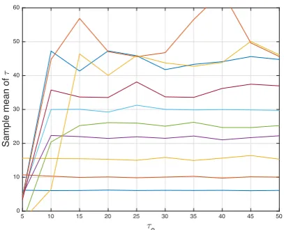
for each posterior. This makes sense from a theoreti-cal point of view since these means arise from the same posterior distribution, for a fixed truth, but it is also re-assuring from a computational point of view since the output is close to independent of the initial guess for the length scale. There does however appear to be an issue with initializing the value of⌧ at too low a value, with the value⌧ tending to get stuck far from the truth when initialized at = 5. This e↵ect has been detected in several other experiments and models – initializing the value of⌧ much lower than the true inverse length can cause the parameter to become stuck in a local min-imum. Such an e↵ect has not been observed however when the parameter is initialized significantly larger than the true value. Table 1 shows that recovery of the true value of ⌧ is very good for ⌧† _{ 35, though} be-comes slightly worse for larger values of⌧†. The means here are calculated without the ⌧0 = 5 sample means since they are clearly outliers for most of the posteriors. One possible explanation for the lack of recovery in the cases ⌧† = 40, 45 and 50 is to do with the structure of the observation map S. The observation grid has a length scale associated with it, related to distances be-tween observation points, and so issues could arise when trying to detect the length scale of the geometric field that is significantly shorter than this. Additionally, the length scales 1/⌧are closer for larger⌧and so it may be more difficult to distinguish between particular values. For brevity we now focus on the case where⌧†= 15. The traces of the values of ⌧ along the hierarchical chains corresponding to this truth is shown in Figure 3. After approximately 106_{samples, all chains have} be-come centered around the true length scale. This con-vergence appears to be roughly linear for each chain.

Figure 4 shows the push forwards of the sample means from the di↵erent chains under the level set map, that is, approximations of F(E(u),E(⌧)). This figure also shows approximations of _E(F(u,⌧)) and typical samples of F(u,⌧) coming from the di↵erent chains. We see that these conditional means for the hierarchi-cal method appear to agree with one other. This is re-assuring for the reason mentioned above – they are all estimates of the mean of the same distribution. The fig-ures for the non-hierarchical posteriors admit greater variation, especially near the boundary for higher val-ues of⌧. Moreover, not all inclusions are detected when the length scale parameter is taken to be⌧ = 5. Note that the mean from the hierarchical posterior agrees closely with that from the non-hierarchical posterior using the fixed true length-scale ⌧ = 15. Additionally, even though the means are reasonable approximations to the truth in most cases, the typical samples are much

worse when using the non-hierarchical method with an incorrect length scale parameter.

We can also consider the sample variance of the pushforward of the samples by the level set map, i.e. ap-proximations of the quantity Var(F(u,⌧)). In Figure 5 we show this quantity for both the hierarchical and non-hierarchical priors. Note that for the non-non-hierarchical priors, the variance increases both at the boundary and away from the observation points for larger values of⌧. Variance is also higher along the interfaces and within the central phase, since points in these locations are more likely to switch between all three phases. The hi-erarchical approximations all appear to agree. Whilst the hierarchical means are very similar to the non-hierarchical means using the true length scale, as seen in Figure 4, the hierarchical variances are smaller away from the observation points.

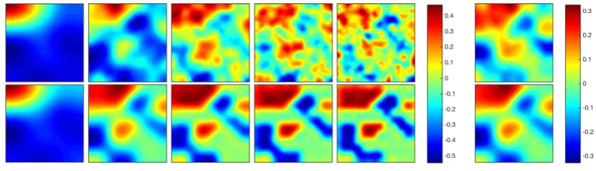
Additionally, we look at the level set functionu it-self in Figure 6. In these plots we rescale the level set function by ⌧↵ d/2 = ⌧4 so that they are all of ap-proximately the same amplitude. The means for both the hierarchical and non-hierarchical methods are again quite similar to one another, though the di↵erence be-tween the typical samples is much more stark.

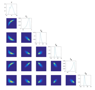
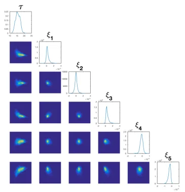
Finally, in Figure 7, we look at the joint densities of the inverse length scale parameter ⌧ and first five Karhunen-Lo`eve (KL) modes of the level set function u.4 _{Non-trivial correlations are evident between⌧ and} each of these modes, with the support of the densi-ties appearing non-convex. This is likely related to the non-linear scaling between the length-scale and the am-plitude of the level-set function under the prior. Con-versely the KL modes, whilst still correlated with one-another other, have simpler joint densities. Note, also, that the posterior on the length scale is centered close to the true value of the inverse length scale parameter

⌧.

τ 0

5 10 15 20 25 30 35 40 45 50

Sample mean of

τ

0 10 20 30 40 50 60

Fig. 2 (Identity model) The sample mean of ⌧ along each hierarchical MCMC chain, against the initial value of⌧. The di↵erent curves arise from using di↵erent datayi.

Table 1 (Identity model) The value of⌧ used to create the data yi, and the mean value of⌧ across the MCMC chains and the di↵erent initial values of⌧.

⌧† _{Mean sample mean of⌧}

5 6.10

10 10.0

15 15.5

20 21.8

25 24.8

30 30.0

35 35.4

40 44.6

45 50.8

50 40.6

generalized linear mixed models, the marginal variance and length-scale parameters of a Mat´ern field cannot be consistently estimated in this limit where as in our case the domain is fixed. This is in contrast to the case of additional data points increasing the domain, where consistent estimation is possible [32]. ut

4.3 Identification of Geologic Facies in Groundwater Flow

The identification of geologic facies in subsurface flow applications is a common example of a large scale in-verse problem that involves the recovery of unknown interfaces. In the case of groundwater flow, for exam-ple, the inverse problem concerns the recovery of the in-terface between regions with di↵erent hydraulic conduc-tivity given measurements of hydraulic head. Geometric

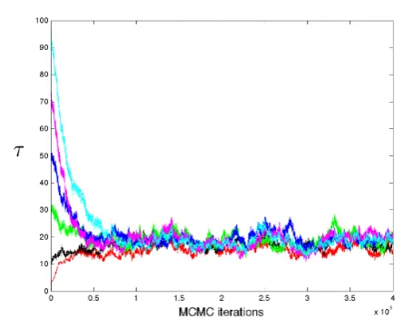
MCMC iterations ×106

0 0.5 1 1.5 2 2.5 3 3.5 4 4.5 5

τ

0 5 10 15 20 25 30 35 40 45 50

Fig. 3 (Identity model) The trace of ⌧ along the MCMC chain, when initialized at the 10 di↵erent initial values. True inverse length scale is⌧= 15.

inverse problems of this type have recently received a lot of attention by the research community [39, 40, 44, 56]. Indeed, it has been recognized that the geometry de-termined by the aforementioned interfaces constitutes one of the main sources of uncertainty that must be quantified and reduced by means of Bayesian inversion. In the context of groundwater flow, the identifica-tion of interfaces between regions associated with dif-ferent types of geological properties can be posed as the recovery of a piecewise constant conductivity field pa-rameterized with a level set function. A fully Bayesian level set framework for the solution of the aforemen-tioned type of inverse problems has been recently de-veloped in [31]. The MCMC method applied in [31] performs well when the prior of the level set function properly encodes the intrinsic length-scales of the un-known interfaces. Clearly, in practical applications such length-scales are most likely unknown and their incor-rect specification may result in inaccurate and uncer-tain estimates of the unknown interfaces. The purpose of this section is to show that the proposed hierarchical Bayesian framework enables us to determine an opti-mal length-scale in the prior of the level set function which, in turn, captures more accurately the intrinsic length-scale of the unknown interface.

4.3.1 The forward model

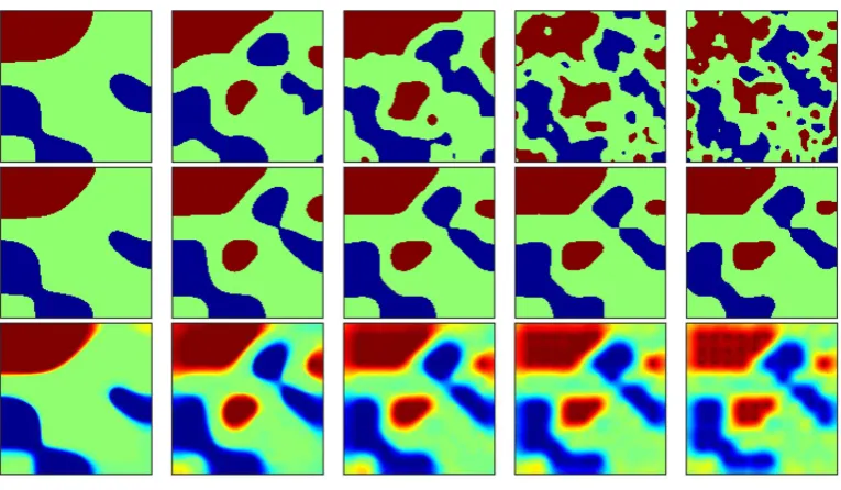
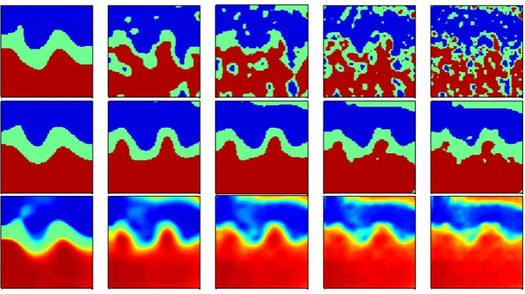
(a) The true geometric field used to generate the datay, with true inverse length scale⌧= 15

(b) (Top) Representative samples ofF(u,⌧) under the hierarchical posterior. (Middle) Approxima-tions ofF(E(u),E(⌧)). (Bottom) Approximations ofE(F(u,⌧)). From left-to-right,⌧ is initialized at

⌧= 5,15,25,35,45.

(c) As in (b), using the non-hierarchical method. From left-to-right,⌧ is fixed at⌧= 5,15,25,35,45.

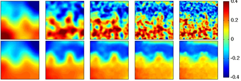
Fig. 5 (Identity model) Approximations of Var(F(u,⌧)) using the hierarchical (top) and fixed (bottom) priors, initialized or fixed at⌧= 5,15,25,35,45, from left-to-right. True inverse length scale is⌧= 15.

Fig. 6 (Identity model) Representative samples⌧4_{·u(top) and sample meansE(⌧}4_{·u) (bottom) of the level set function.} The rescaling⌧4 _{means that the above quantities have the same approximate amplitude. True inverse length scale is⌧= 15.} (Left) Using the non-hierarchical method; from left-to-right⌧is fixed at⌧= 5,15,25,35,45. (Right) Corresponding quantities for the hierarchical method.

modeled by the solution of [6]

r·rh=f in D (12)

where f represents sources/sinks and where boundary conditions need to be specified. For the present work we consider the setup from the Benchmark used in [14,27– 31]. In concrete, we assume that f is a recharge term of the form

f(x1, x2) = 8 < :

0 if 0< x24, 137 if 4< x2<5, 274 if 5_x2<6.

(13)

and we consider the following boundary conditions

h(x1,0) = 100, @h

@x1

(6, x2) = 0,

@h @x1

(0, x2) = 500, @h

@x2

(x1,6) = 0.

(14)

We consider the inverse problem of recovering 

from observations _{`j(h)}64j=1 of h given by (12)-(14).

We assume we have smoothed point observations given by

`j(h) = Z

D 1 2⇡"2e

1

2"2(x qj)2_{h(x) dx}

where">0 and_{qj_}64

j=1✓Dis a grid of 64 observation points equally distributed on D. Let Z = Lp_{(D) for} some 1p <1and Y =R64_{. Given2Z, leth be} given by (12)-(14). Then the forward mapS :Z _!Y is given by

_7!(`1(h), . . . ,`64(h)).

Fig. 7 (Identity model) (diagonal) Empirical densities of⌧ and the first five KL modes of u. (o↵-diagonal) Empirical joint densities. True inverse length scale is⌧= 15.

4.3.2 Simulations and results

In the previous example we illustrate, with a simple model, the capabilities of the proposed framework to recover a specified true length-scale and a true level set function that defines a true discontinuous field from which synthetic data are generated. However, we must reiterate that, in practice, we wish to recover the true discontinuous field; the level set function is merely an artifact that we use for the parameterization of such a field. In practical applications the aim of the proposed hierarchical Bayesian level set framework is to infer a length-scale alongside with a level set function which, by means of expression (7), produces a discontinuous field that captures the desired piecewise constant field as accurately as possible and, in particular, the intrinsic length-scale separation of the interfaces determined by

Synthetic data are generated by means of y= (`1(h†), . . . ,`64(h†)) +⌘, ⌘_⇠N(0, ) i.i.d. whereh† _{is the solution to (12)-(14) for =}†_. Equa-tions (12)-(14) have been solved with cell-centered finite di↵erences [5]. In order to avoid inverse crimes, syn-thetic data are generated on a grid finer (160⇥160 cells) than the one used for the inversion (80_⇥80 cells). The discretization is performed via the DFT, and we retain all modes. In addition, is a diagonal matrix given by i,i = 0.0175`i(h†). In other words, we add noise that corresponds to 1.75% of the size of the noise-free obser-vations. On the prior for the level set functionuwe take Neumann boundary conditions and fix the smoothness parameter ↵= 5.

We consider a Gaussian priorN(35,102_{) for⌧, and} use a Gaussian random walk proposal distribution for this parameter. We then apply the hierarchical MCMC method from subsection 3.3 initialized with the follow-ing six di↵erent choices of ⌧ = 1,10,30,50,70,90 and a sample of the prior (with that given ⌧) of the level set function u. We thus produce six MCMC chains of length 4⇥106 and discard the first 106 as burn-in for the computation of quantities of interest. The trace plots of ⌧ are displayed in Figure 8 from which we clearly observe that all chains, regardless of their initial point, seem to stabilize and produce samples around

⌧ = 18. In the top row of Figure 9(b) we display the logarithm of some representatives samples of F(u,⌧) under the hierarchical posterior. The middle row of Figure 9(b) shows the logarithm of F(E(u),E(⌧)), i.e., the pushforward of the posterior means obtained us-ing the hierarchical method. The bottom row of Figure 9(b) displays the logarithm of the approximations of

E(F(u,⌧)). That is, the expected value of the pushfor-ward samples under the posterior. The aforementioned results corresponds to five MCMC chains with ⌧ ini-tialized⌧ = 10,30,50,70,90 (the results for⌧ = 1 have been omitted). Similarly, Figure 10 (top) shows the ap-proximations of the variance of the pushforward sam-ples of the posterior, i.e. Var F(u,⌧) . Clearly, both

E(F(u,⌧)) and F(_E(u),_E(⌧)) result in fields that pro-vide a reasonable approximation of the true geometric field. Note that, as expected, the largest uncertainty in the distribution of the pushforward samples is around the interface between the regions with di↵erent con-ductivity. In Figure 11(a) we show some representative samples of u (top) and approximations to E(u) (bot-tom). In these plots, as before, we rescale the level set function by⌧↵ d/2_=⌧4 _{so that they are all of} approx-imately the same amplitude. In Figure 12 we display the empirical densities of⌧and the first five KL modes of u. A key observation is that, although the true

hy-draulic conductivity is not generated by thresholding a Gaussian random field, and hence there is no “true” length scale, the posterior nonetheless settles on a nar-row range of values of⌧ which are consistent with the data.

From the aforementioned results we can also clearly see that the hierarchical MCMC algorithm produces similar outcomes regardless of the initialization of the inverse of the length-scale⌧, reflecting ergodicity of the Markov chain. The results from⌧ = 1 are not shown but they are very similar to the ones from other chains. As with the results from the previous subsection, the simi-larity in outcomes between all six chains is not surpris-ing as these are aimed at samplsurpris-ing from the same poste-rior distribution; but the fact that this posteposte-rior distri-bution on⌧ concentrates near to a single value is of par-ticular interest because it shows that the true geometric field has an intrinsic length-scale, even though it was not constructed via the mapF(u,⌧).Furthermore, this similarity of outcomes between chains showcases the main advantage of the proposed framework with respect to the non-hierarchical one. Indeed, as stated earlier, the proposed method has the ability to recover a distri-bution for the intrinsic length-scale which gives rise to reasonably accurate estimates (i.e. F(_E(u),_E(⌧)) and

E(F(u,⌧))) of the true geometric field. We now present the numerical results from applying a non-hierarchical MCMC algorithm in which the inverse of length-scale⌧

is fixed. We consider again six MCMC chains as before with the (now fixed) values of ⌧ = 1,10,30,50,70,90 that we used to initialized the hierarchical chains used before. Analogous results to the ones presented for the hierarchical method can be found in the bottom pan-els of Figure 9 as well as the bottom of Figures 10 and 11. Clearly, the lack of properly prescribing the intrin-sic length-scale in the non-hierarchical method results in inaccurate estimates of the true geometric field. We clearly observe that for ⌧ 30 the estimates of the truth given by F(E(u),E(⌧)) and E(F(u,⌧)) are sub-stantially inaccurate and the uncertainty measured by Var F(u,⌧) is large. The non-hierarchical MCMC for

⌧= 1 did not converge; the results are not shown. The non-hierarchical MCMC only provides reasonable esti-mates for⌧ = 10 and⌧= 30. However, we can visually appreciate that these results are still suboptimal when compared to the results from the hierarchical frame-work.

4.4 Electrical Impedance Tomography

Fig. 8 (Groundwater flow model) Trace plots of⌧ obtained from six hierarchical MCMC chains.

method [20]. In this subsection we show that the hi-erarchical approach outperforms the non-hihi-erarchical approach in the case where the true conductivity is a binary field, given the same number of forward model evaluations.

4.4.1 The forward model

EIT is an imaging technique which attempts to infer the internal conductivity of a body from boundary volt-age measurements. Typical applications include medi-cal imaging, as well as subsurface imaging where it is known as electrical resistivity tomography (ERT). We utilize the complete electrode model (CEM), proposed in [49]. This is a physically accurate model which has been shown to agree with experimental data up to mea-surement precision. The strong form of the PDE gov-erning the model is given by

8 > > > > > > > > > > < > > > > > > > > > > :

r·((x)_rv(x)) = 0 x₂D Z

el

@v

@ndS=Il l= 1, . . . , L

(x)@v

@n(x) = 0 x2@D\ SL

l=1el

v(x) +zl(x)@v

@n(x) =Vl x2el, l= 1, . . . , L. HereD_✓R2_{is the domain and}

{el_}L

l=1✓@D are elec-trodes on the boundary upon which currents{Il}L

l=1are injected and voltages _{Vl_}L

l=1 are read. The numbers {zl_}L

l=1 represent the contact impedances of the elec-trodes. The field  represents the conductivity of the body and v represents the potential within the body5. 5 _{In the EIT literature the conductivity field is often} de-noted , however we have already used this in denoting the marginal variance of random fields.

It should be noted that the solution of this PDE com-prises both a potentialv2H1_{(D) and a vector{Vl}}L

l=1 of boundary voltage measurements.

The inverse problem we consider is the recovery of

from a sequence of boundary voltage measurements. A number of (linearly independent) current stimulation patterns_{Il_}L

l=1 may be performed to provide more in-formation; we assume that we perform the maximum M = L 1 measurements. Let Z = Lp_{(D) for some} 1 _ p < ₁ and Y = _RJ _{where J = LM. We can} concatenate the boundary voltage measurements aris-ing from di↵erent stimulation patterns to yield a map S:Z _!Y,

_7!(V(1)_{, V}(2)_{, . . . , V}(M)₎

whereV(m)₌

{V_l(m)_}L

l=12RL,m= 1, . . . , M.

For the experiments we work on a circular domain D = _{x _{2 R}2

| |x_| < 1_}. 16 electrodes are spaced equally around the boundary providing 50% coverage. All contact impedances are taken to bezl= 0.01. Adja-cent electrodes are stimulated with a current of 0.1, so that the matrix of stimulation patternsI={I(j)_}15

j=12

R16⇥15_{is given by}

I= 0.1_⇥ 0 B B B B B B @

+1 0 _{· · ·} 0 1 +1 · · · 0

0 1 . .. 0

..

. ... . .. +1

0 0 0 1

1 C C C C C C A .

We define our forward map_G:X_⇥R+

!RJ_by G= S F. As in the groundwater flow example, assume that eachi in the definition of the level set map is strictly positive. We do not have a continuity result for the map S on Lp _{for any 1p <1. However the almost-sure} continuity of the map_G can be seen via a modification of the proof of Proposition 3.5 in [20] to include the parameter ⌧; this modification is almost identical to the proof of Proposition 1 given in the appendix. The uniform boundedness of_G follows from a result in [20] similarly. Hence as was the case with the identity map example, the conclusions of Proposition 1 follow, and we can deduce the conclusions of Theorem 2.

4.4.2 Simulations and results

We fix a true conductivity†_{, shown in Figure 14. As} with the groundwater flow experiments, this is con-structed explicitly and does not have a true value of

0 1 2 3 4 5 6 0

1 2 3 4 5 6

1.5 2 2.5 3 3.5 4 4.5 5 5.5 6 6.5

(a) (Left) Logarithm of the true hydraulic conductivity field used to generate the data y. (Right) True pressure field, and the grid of observation points.

(b) (Top) Logarithm of representative samples ofF(u,⌧) under the hierarchical posterior. (Middle) Logarithm of the approximations of F(E(u),E(⌧)). (Bottom) Logarithm of the approximations of E(F(u,⌧)). From left-to-right,⌧ is initialized at⌧= 10,30,50,70,90.

(c) As in (b), using the non-hierarchical method. From left-to-right,⌧is fixed at⌧= 10,30,50,70,90.

Fig. 10 (Groundwater flow model) Approximations of Var F(u,⌧) using the hierarchical (top) and the non-hierarchical (bottom) MCMC.

(a) (Top) Representative samples of the rescaled level-set function⌧4_{·uand (bottom) approximations} ofE(⌧4_{·u) using the hierarchical method. From left-to-right,⌧is initialized at⌧= 10,30,50,70,90.}

(b) As in (a), using the non-hierarchical method. From left-to-right,⌧ is fixed at⌧= 10,30,50,70,90.

Fig. 12 (Groundwater flow model) (diagonal) Empirical densities of⌧and the first five KL modes ofu. (o↵-diagonal) Empirical joint densities.

where we take the noise covariance = 0.00022

·Ito be white. The mean relative error on the generated data is approximately 12%. The data is generated using a mesh of 43264 elements and simulations are performed used a mesh of 10816 elements, in order to avoid an inverse crime. Forward solves are performed using the EIDORS software [1]. All level set field samples are defined on the square [ 1,1]2 _{and restricted to the domain D. This} has the advantage of allowing for efficient sampling via the Fast Fourier Transform, though has the drawback of introducing possibly non-trivial boundary e↵ects on the domain; no such e↵ects are observed in our problem, however. The discretization on the square is performed via the DFT on a grid of 27_⇥27_{points, and we retain} all modes.

The level set map F is defined such that there are 2 phases, taking the constant values 1 and 10. We take the prior level set field mean to be zero, so that in this caseF (and hence ) becomes independent of⌧. Thus a forward model evaluation is not required for the Gibbs update of⌧, and each sample of (u,⌧) using the hierar-chical method costs virtually the same as one ofuusing the non-hierarchical method.

wish to compare how the hierarchical method compares with the non-hierarchical method. We therefore also look at the 5 di↵erent posterior distributions that arise when using each of 5 fixed prior inverse length scales

⌧ = 10,30,50,70,90, which gives another 5 MCMC chains. For both the methods we produce 4_⇥106 sam-ples for each chain, and discard the first 2_⇥106_samples as burn-in when calculating quantities of interest.

The traces of the values of ⌧ along the hierarchi-cal chains are shown in Figure 13. With the exception of the chain initialized at ⌧ = 10, the chains converge to the sample approximate value of ⌧. Unlike in pre-vious experiments, the traces have a relatively flat pe-riod before the approximate linear convergence to the common length scale. Initializing ⌧ = 90 requires an additional 106_{samples to converge, over the other} con-verging chains.

Figure 14 shows the push forwards of the sample means from di↵erent chains under the level set map, along with approximations of E(F(u,⌧)) and typical samples ofF(u,⌧) coming from the di↵erent posteriors. In both the hierarchical and non-hierarchical methods, the chains initialized/fixed at⌧ = 10 fail to recover the true conductivity, similarly to what was observed with the identity map experiments when initializing at⌧= 5. The other chains for the hierarchical method produce very similar results to one another, whilst the e↵ect of fixing the length scale to be too short is apparent in the figures for the non-hierarchical method.

In Figure 15 we see approximations to Var(F(u,⌧)) under the di↵erent posteriors. In both cases, variance is highest around the boundaries of the two inclu-sions. The di↵erence between the hierarchical and non-hierarchical methods is more apparent here, with higher variance between the two inclusions when the length scale is fixed to be too short.

Again, we look at the level set function u itself in Figure 16. In these plots, as before, we rescale the level set function by ⌧↵ d/2 = ⌧4 so that they are all of approximately the same amplitude. As in the previous experiments, there is noticeable contrast between the means for the hierarchical and non-hierarchical meth-ods, and yet more contrast between the typical samples. Finally, in Figure 17, we show the posterior densi-ties on the inverse length scale and the first five KL modes, as well as correlations between them. As with the groundwater flow example, although there is no “true” inverse length scale, the data is sufficiently in-formative to define a small range of values for this pa-rameter under the posterior.

MCMC iterations _×106

0 0.5 1 1.5 2 2.5 3 3.5 4

τ

0 10 20 30 40 50 60 70 80 90

Fig. 13 (EIT model) The trace of⌧along the MCMC chain, when initialized at the 5 di↵erent values⌧= 10,30,50,70,90.

5 Conclusions

The level set method is an attractive approach to in-verse problems for the detection of interfaces. Further-more the Bayesian approach is particularly desirable when there is a need to quantify uncertainty. In this paper we have shown that Bayesian level set inversion is considerably enhanced by a hierarchical approach in which the length scale of the underlying level set func-tion is inferred from the data. We have demonstrated this by means of three examples of interest arising in, respectively, the information, physical and medical sci-ences; however many potential applications remain to be explored and this provides an interesting avenue for future work.

We also developed the theoretical underpinnings for our hierarchical method. Our work is based on a Metropolis-within-Gibbs approach which alternates be-tween updating the level set function and the length-scale. The Metropolis method we use for the level set field update does not use derivatives of the log-likelihood, and could be improved by doing so, using the infinite dimensional variants on MALA and HMC (which use first derivative information, see the citations in [16]) or the manifold MALA and HMC methods, which use higher order derivatives [25]. Another inter-esting direction for future work is the design of meth-ods with more informed proposals which exploit cor-relations in the level set function and its length-scale. And finally it would be interesting to consider pseudo-marginal methods to sample the hierarchical parameter alone, as in [21].

1 10

j

0 50 100 150 200 250 yj

-0.06 -0.04 -0.02 0 0.02 0.04 0.06

(a) (Left) True conductivity field used to generate the data y. (Right) The entries yi of the data vectory, plotted againsti.

(b) (Top) Representative samples ofF(u,⌧) under the hierarchical posterior. (Middle) Approxima-tions ofF(E(u),E(⌧)). (Bottom) Approximations ofE(F(u,⌧)). From left-to-right,⌧ is initialized at

⌧= 10,30,50,70,90.

(c) As in (b), using the non-hierarchical method. From left-to-right,⌧is fixed at⌧= 10,30,50,70,90.

20

0 10

Fig. 15 (EIT model) Approximations of Var(F(u,⌧)) using the hierarchical (top) and fixed (bottom) priors, with⌧initialized or fixed at⌧= 10,30,50,70,90, from left-to-right.

(a) (Top) Representative samples of the rescaled level-set function⌧4_{·uand (bottom) approximations} ofE(⌧4_{·u) using the hierarchical method. From left-to-right,⌧is initialized at⌧= 10,30,50,70,90.}

(b) As in (a), using the non-hierarchical method. From left-to-right,⌧ is fixed at⌧= 10,30,50,70,90.

Fig. 16 (EIT model) Representative samples and sample means of the level set function. The rescaling⌧4 _{means that the} above quantities have the same approximate amplitude. True inverse length scale is⌧= 15.

part of the inference as well; we omitted this here for the sake of clarity. Such a model may be more realistic, and numerical studies of such models may prove interesting. Another extension of interest may be to place a hyper-prior upon the regularity parameter also, which may be useful for improving rates of convergence [54]. This is a more challenging task, again related to singularity of