Optical fibres in pre detector signal processing

ZIRCONIA-BASED ELECTROCERAMIC MATERIALS FOR

SOFC APPLICATIONS

Alan John Feighery

A Thesis Submitted for the Degree of PhD

at the

University of St Andrews

1999

Full metadata for this item is available in

St Andrews Research Repository

at:

http://research-repository.st-andrews.ac.uk/

Please use this identifier to cite or link to this item:

http://hdl.handle.net/10023/13601

\\Bm

Optical fibres in pre-detector signal processing

A thesis presented by

A R P lin n B S c AUS

to the

University of St Andrews

in application for the degree of

Doctor of Philosophy

ProQuest Number: 10166557

All rights reserved INFORMATION TO ALL USERS

The quality of this reproduction is d e p e n d e n t u p on the quality of the co p y subm itted. In the unlikely e v e n t that the author did not send a c o m p le te m anuscript

and there are missing p a g e s , these will be n o ted . Also, if m aterial had to be rem o v ed , a n o te will in d icate the d eletio n .

uest

ProQ uest 10166557

Published by ProQuest LLO (2017). C opyright of the Dissertation is held by the Author. All rights reserved.

This work is protected a g a in st unauthorized copying under Title 17, United States C o d e Microform Edition © ProQuest LLO.

ProQuest LLO.

789 East Eisenhower Parkway P.Q. Box 1346

XV-Certificate

I certify th a t A R Flinn BSc AUS has spent nine term s a t research work in the Physical Sciences Laboratory of St Salvador's college, in the University of St Andrews, under my direction, th at he has fulfilled the conditions of Ordinance No 16 (St Andrews) and th a t he is qualified to submit the thesis in application for the degree of Doctor of Philosophy.

A M aitland

Declaration

I hereby certify th at this thesis has been composed by me, and is a record of work done by me, and has not previously been presented for a higher degree.

This research was carried out in the Physical sciences laboratory of St Salvador's college, in the University of St Andrews, under the supervision of Dr A M aitland.

A R Flinn

Acknowledgements

I would like to th an k Dr. A rthur M aitland for. his guidance and encouragem ent throughout this work. I am grateful to A dm iralty Research Establishm ent for financial support and to my industrial supervisors Prof. H erbert French and Dr. Phil Sutton for their help, interest and not least, enthusiasm for the project.

Thanks also to all Physics postgrads, past and present, for m aking life enjoyable inside and outside the departm ent, above and below 3000ft, especially, the m erry band of L aser 1, Callum , M iles, Graham , Liz, and everone nam ed Andy!

I would like to thank Denise, my wife, for her patience particularly during the later stages of the work.

A uthor's career

Contents

Sssâsm

TWs.

Abstract

1

1

Introduction

4

1.1 Electro-optic sensors 4

1.2 Pre-detector signal processing 5

1.3 Optical fibres 6

1.4 Fibre optics 7

1.5 Pre-detector signal processing with optical fibres 9 1.6 Optical Signal Processing with Optical Fibres 10

2

Theory

14

2.1 Waveguide theory 14

2.1.1 The step-index optical fibre - ray model 17 2.2 The step-index optical fibre - wave model 19

2.2.1 The step-index optical fibre 19

2.2.2 Linearly polarised modes 24

2.2.3 Number of modes in a step-index fibre 24 2.3 Group dispersion in a step-index fibre 26

2.3.1 M aterial Dispersion 29

2.3.2 Interm odal Dispersion 30

2.4 Phase Dispersion in a step-index fibre 33

2.4.1 Optical Path Length 36

2.5 Interference 38

2.5.1 W avefront splitting interferom eters 40 2.5.2 Amplitude splitting interferom eters 42

2.6 Coherence Theory 45

2.6.1 The Analytic Signal 47

2.6.2 Coherence as defined by correlation integrals 49

Section Title

_Eaa

3

Background and Review

58

3.1 Fibre optic interferom etric sensors 58

3.2 Phase Modulation 61

3.3 Interferom etric arrangem ents 62

3.3.1 Young's Slits interferom eters 62

3.3.2 Mach-Zehnder interferom eter 62

3.3.3 Michelson interferom eter 63

3.4 Multimode Optical Fibre Interferom etry 63

3.4.1 Multimode Fibres in Astronomy 66

3.5 Coupling Light into Optical Fibre 67

3.6 Scalar Diffraction Theory

70

3.6.1 Region of Fresnel Diffraction 72

3.6.2 Region of Fraunhofer Diffraction 73

3.7 Fourier optics 75

3.7.1 The phase shifting properties of a lens 75 3.7.2 The Fourier transform ing properties of a lens 76

3.8 Spatial coherence filtering 79

3.8.1 Convolution w ith incoherent and coherent

illum ination 79

3.8.2 Image formation with incoherent illumination 79 3.8.3 Image formation with coherent illum ination 81 3.8.4 image formation with partially coherent

illum ination 81

3.8.5 Spatial coherence filtering with coherent and

incoherent sources 84

3.8.6 Spatial coherence functions 86

3.9 Spectral filtering 87

3.10 Temporal coherence filtering 88

3.10.1 Temporal filtering with a Gaussian spectral profile 89

B edim . lifle.

4

Experimental

92

4.1 Young's slits interference patterns 92 4.1.1 Multiple beam interference patterns 95 4.2 Mach-Zehnder type interference patterns 96

4.3 Phase front maps 98

4.4 M easurem ent of visibility curves by fibre interferom eter 99 4.5 Optical fibre bandpass coherence filtering 101

4.6 Coherence spectrometer 103

4.7 Optical fibre couplers 105

4.8 Coherence In Optical Fibres 109

4.8.1 Temporal Coherence In Fibres 112

4.8.2 Spatial Coherence In Optical Fibres 113 4.8.3 Coherence In Optical Fibres - experimental 116 4.8.4 An Interferom eter and an optical fibre as an Optical

Filter 119

5

Experimental

122

5.1 Fibre arrays 122

5.1.1 Correlation of interference fringes with a ID fibre array 124 5.1.2 Correlation of radiation across a scene 125 5.1.3 M easurem ent of path difference across a scene 126

5.2 Scanning light over fibres 127

5.2.1 Scanning a Fourier transform image over a single fibre 127

5.2.2 Scanning light over two fibres 129

5.3 Spatial coherence sensors. 129

5.4 The spatial light modulator known as SIGHT-MOD. 135

5.7.1 Control of the SIGHT-MOD 136

5.7.2 The SIGHT-MOD as a fibre optic switch 137

5.7.3 Contrast of SIGHT-MOD 138

5.7.4 Fourier transform s of gratings produced by the

SIGHT-MOD 140

5.7.5 M anipulation of Fourier transform images using a fibre

array 141

5.7.6 Correlation of linear interference fringes w ith gratings

BesMm

TMM.

6

EHscussion : Pre-detector signal processing 145

optical fibres 146

6.2 Discussion of coherence in fibres 149

6.3 Discussion of fibre arrays 151

6.4 W avelength demultiplexing 153

6.6 Discussion of fibre interferom eters 154

6.7 Discussion of SIGHT-MOD 155

6.8 Conclusions 156

References

156

Appendix A : Waveguide Theory 161

Appendix B : Gaussian beam optics for a singlemode fibre 165 Appendix C : Visibility curve obtained for a Lorentzian

spectral profile 168

Appendix D : The Fourier transform of a ID grating 169

IV

Abstract

The basic form of conventional electro-optic sensors is described. The m ain drawback of these sensors is their inability to deal w ith the background radiation which usually accompanies the signal. This 'clutter' lim its the sensors performance long before other noise such as 'shot' noise. Pre-detector signal processing using the complex am plitude of the light is introduced as a m eans to discrim inate betw een the signal and 'clutter'. F u rth er im provem ents to p re­ detector signal processors can be made by the inclusion of optical fibres allowing radiation to be used w ith greater efficiency and enabling certain signal processing tasks to be carried out w ith an ease unequalled by any other method.

The theory of optical waveguides and their application in sensors, interferom eters, and signal processors is reviewed. Geom etrical aspects of the form ation of linear and circular interference fringes are described along w ith tem poral and spatial coherence theory and their relationship to Michelson's visibility function.

The requirem ents for efficient coupling of a source into singlemode and m ultim ode fibres are given. We describe in terferen ce experim ents between beam s of light em itted from a few m etres of two or more, singlemode or multimode, optical fibres.

Correlations between laser light from different points in a scene is investigated by interfering the light em itted from an array of fibres, placed in the image plane of a sensor, with each other. Temporal signal processing experiments show th at the visibility of interference fringes gives inform ation about p ath differences in a scene or through an optical system.

M ost E -0 sensors employ w avelength filtering of the detected radiation to improve their discrimination and this is shown to be less selective th an tem poral coherence filtering which is sensitive to spectral bandw idth. E xperim ents using fibre interferom eters to discrim inate between red and blue laser light by their bandw idths are described. In m ost cases the path difference need only be a few tens of centimetres.

We consider spatial and tem poral coherence in fibres. We show th a t high visibility interference fringes can be produced by red and blue laser light transm itted through over 100 m etres of singlemode or multimode fibre. The effect of detector size, relative to speckle size, is considered for fringes produced by multimode fibres. The effect of

2

1 using optical transfer functions which are sensitive to the spatial i coherence of the illum inating light. Spatial coherence sensors which

use gratings as aperture plane reticles are discussed.

dispersion on the coherence of the light em itted from fibres is considered in term s of correlation and interference between modes.

We describe experim ents using a spatial light m odulator called SIGHT-MOD. The device is used in various systems as a fibre optic switch and as a programmable aperture plane reticle. The contrast of the device is m easured using red and green, HeNe, sources. Fourier transform im ages of p attern s on the SIGHT-MOD are obtained and used to dem onstrate the geometrical m anipulation of im ages using 2D fibre arrays. C orrelation of Fourier transform images of the SIGHT-MOD with 2D fibre arrays is demonstrated.

3

1 Introduction

LI Electro-optic sensors.

Remote sensing may be defined as the detection of electromagnetic (EM) radiation emitted, reflected, or scattered from an object. The EM radiation from an object together w ith the EM radiation from the background is detected by an electro-optic (EO) sensor. The EO sensor converts the optical signal into an electrical signal. The task of the EO sensor is to m easure the radiation from the object, i.e. the signal, in the presence of background radiation.

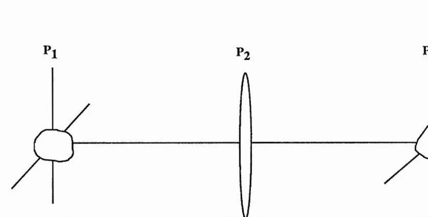
W ith the exception of heterodyne systems nearly all EO sensors have the general form shown in figure 1.1. They collect light from a scene using some combination of reflecting or refracting optics and then bandlim it the light by m eans of a spectral filter. The filter is chosen so as to maximise the ratio of signal to background radiation. The sensor can be imaging in which case the intensity is m easured by a 2D detector array, figure 1.2a, or the scene is scanned over a small num ber of detectors. Alternatively, the sensor may be non-imaging, in which case it can only detect power in a determ ined waveband, figure 1.2b. Both the signal and background rad iatio n can be m odulated by a rotating reticle in the detector plane in order to aid the post-detector electronic processing. Signal processing aim s to improve the discrim ination betw een the signal and the unw anted background in a scene.

circuits, we can study the image quality of an optical system by applying frequency response techniques, usually w ith the aid of tran sfer functions. Exam ples of lin ear processes are bandpass filtering, subtraction, convolution and correlation. In an optical system the detected output is always an intensity. W ith incoherent light, the input and output intensities have a linear relationship. W ith coherent light, the input and output are based on amplitude and intensity, respectively, so their relationship is no longer linear.

L2 Pre-detector signal processing.

Signal processing m ay be carried out before or after square-law detection so we have the option of pre-detector or post-detector processing. The discrim ination of E -0 sensors which use post­ detector processing is often poor because they have to discrim inate between signal and background on the basis of intensity as all phase inform ation is lost in the square-law detection process. Problems arise when the intensity of the background radiation approaches th at of the signal. Pre-detector processing can take advantage of this phase and amplitude information which can give information about the spectrum , coherence, and polarisation of the light by selective modulation of these param eters prior to electronic detection [1.1].

and so exhibit a high degree of spatial coherence compared w ith norm ally diffuse background rad iatio n . O ptical pre-detector processing may be employed to take advantage of these differences in spatial coherence.

Pre-detector signal processing techniques can take advantage of polarisation differences between a source and background radiation. Laser sources are often highly linearly polarised but therm al sources are usually unpolarised. Features such as clouds reflect light which is elliptically polarised so a form of polarisation m odulation may discrim inate between differently polarised radiations.

Pre-detector optical signal processing techniques often m ake use of the Fourier transform . This branch of signal processing is known as Fourier Optics and is described in detail by Goodman [1.2], Steward [1.3], and Bracewell [1.4]. O ther transform s m ay be perform ed optically, for example, the H artley transform [1.5], and the Sine and Cosine transform s [1.6].

Optical fifeyesi

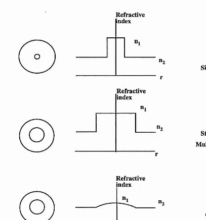
Optical fibres are waveguides made of transparent m aterials such as silica glasses which can tran sm it visible and infra-red light over long distances w ith low loss (> 0.2 dB/km a t 1500nm). An optical fibre consists of an inner core which guides the light and an outer layer, called the cladding, of lower refractive index th an the core. The fibre is usually covered w ith a protective sheath. The refractive indices of the core and cladding, % and ng respectively, can be uniform with a sharp boundary between the two, or there can be a gradual transition in which n i decreases to ng. The two types of fibre are called step- index and graded-index, respectively, figure 1.3.

For a wave to be guided by the fibre it is necessary for it to be totally internally reflected at the core-cladding boundary. Consequently, the light m ust enter the fibre core w ithin a range of angles forming a solid cone. The solid h alf angle of the cone is known as the acceptance angle of the fibre and is related to the refractive indices of the core, cladding, and surrounding medium (usually air for which n=l). We define the num erical aperture of a fibre as the sine of the acceptance angle for the fibre.

Each mode of a step-index multimode fibre propagates a t a slightly different velocity along the axis of the fibre and this causes dispersion and modal noise. If the core diam eter is decreased the num ber of modes decreases until, at wavelengths below a certain critical value, only one mode will propagate. A fibre in which only one mode propagates is called singlemode and has a core diam eter, typically, in the range 3-5 microns.

1*4 Fibre optiia

Fibre optics encompasses all the optics necessary to a system based around optical fibres. A fibre optic signal processing system consists of light from a source coupled into an optical fibre or optical fibre array. The fibres either transm it the light to a signal processing system w ith a predeterm ined geom etry or carry out the signal processing by splitting or combining the light w ith predeterm ined delays betw een the beams. The intensity of the processed optical signal is detected at the output of the system.

We consider the sources, coupling of radiation from the sources into the fibre, and the splicing of two fibres together. We then consider optical fibre directional couplers or splitters and detectors for optical fibre systems.

The source w avelengths typically used in optical fibres are determ ined by the wavelength dependent losses of the fibre itself, figure 1.4. These losses include ultraviolet and infra-red absorption, and R ayleigh sc a tte rin g w hich is caused by d en sity and compositional variation w ithin the fibre. Another source of losses is

% t

due to absorption by dopant and im purity ions such as transition elem ents and the hydroxyl ion from w ater. For high bandw idth communications the wavelength dependent dispersion of the fibre determ ines the maximum permissible linewidth of the source.

Factors which affect the coupling of a source into an optical fibre include unintercepted illum ination. This includes light which is not incident on the entrance to the core of the optical fibre due to an incorrect source spot size. Also, there may be num erical aperture loss. This is caused by th at p art of the source profile th a t falls outside of the fibre acceptance cone. To avoid this, m any integrated optical components have a fibre 'pigtail' perm anently mounted and properly aligned which may then be spliced to another cable. As the core of a monomode fibre is only a few m icrons in diam eter, a slight inaccuracy in alignm ent a t a joint can severely increase the losses, so most joints m ust be spliced.

Two basic methods are used to perm anently join two fibres together. The most widely used is fusion splicing or welding in which the two ends of the fibres are heated, possibly by an electric arc, causing them to soften and fuse together. By this method, losses of less than 0.1 dB have been obtained. A second method of perm anently joining two fibres is to use an adhesive. This generally involves using some additional elem ent to enable the fibres to be accurately aligned for bonding.

10

optics th a t b eam sp litters play in conventional optics. M ost singlemode couplers use evanescent or field coupling. In evanescent

coupling energy is transferred from one optical fibre to another by | virtue of the electric field overlap between the two cores.

L5 Pre-detector sififnal processing with optical fibres.

The introduction of optical fibres into pre-detector signal processing system s allows particular signal processing tasks to be performed which cannot be easily achieved using free space paths, w hilst retaining the ability to discrim inate between signal and background radiation on the basis of phase and amplitude. One of the sim plest tasks which may be considered is th a t of using a few optical fibres to sample the radiation at different points in the image of a scene. The radiation em itted by each fibre m ay be introduced to the same or different signal processing system s. U sing fibre couplers, the radiation from each point may be processed in several ways.

Optical fibres can perform a spatial transform ation. Radiation in an image plane may be guided through an array of fibres and by altering the relative positions of each fibre a new encoded image is produced.

The fibres can perform signal processing by delaying one beam with respect to another as in a fibre interferom eter. The use of optical fibres as delay lines allows the tem poral correlation of radiation in two or more fibres to be carried out with any required time delay. An advantage of fibre paths is th at correlations may be sought between closely or widely separated points in an image with equal ease.

L6 QpticalSignal Processing with QpticalJFibres.

Optical fibres are used in optical signal processing and some of the applications are discussed below.

In 1966 Leith [1.7] described holographic imagery through a diffusing media. By obtaining the phase conjugate of the diffusing media the

object may be reconstructed. In 1976 Leith and Chang [1.8] applied J the same process to a fibre bundle. The phase conjugate of the bundle

A paper by Y oungquist, et al. [1.10] dem onstrated coherence synthesis using an acousto-optic (AO) cell. The visibility curve or coherence function of a source is given by the modulus of the Fourier transform of the spectrum . So if the laser frequency is doppler shifted by the AO cell and then mixed with itself in an optical fibre a new spectrum exists and the coherence function is modified. An array of interferom eters, which have the sam e source, m ay be constructed from optical fibre. If each interferom eter has a different p ath difference then one interferom eter m ay be selected and the others turned off by generating a coherence function which is unity for the path difference of the desired interferom eter and zero for the others.

Optical fibres can be used as an alternative to metallic waveguides in m any microwave system s by m odulating an optical source. Most rad ar systems have a bandw idth of around lOMhz and a singlemode optical fibre w ith a source near the dispersion m inim um can carry a signal w ith a 20Mhz bandw idth 50km. Fibres can be used in optical signal processing systems such as optical delay lines [1.11]. Even allowing for dispersion tim e-bandwidth products of greater th an 10® have been achieved compared w ith 10^-10^ for acoustic wave delay lines. The delay lines may be used for storing received rad ar pulses for re-transm ission or w ith a non-coherent rad ar moving targ et indicator a returned signal is stored for subtraction from the next retu rn [1.12]. Tapped delay lines w ith partially reflecting splices have been dem onstrated by Jackson, et al. [1.13]. These can be used as a bandpass or m atched filter or for pulse compression in high reso lu tio n ra d a rs. U n fo rtu n ately , these tap s are not yet program m able.

If

fi.

Ill

III

i §

îiii

II

I

PQ

I

I

it!

i

I

1

i

₁

I

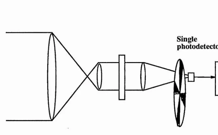
Image plane

2D detector array

Electronic processing Spectral

filter

Input optics

Figure 1.2a Conventional E-O sensor using reflecting input optics

and a 2D detector array in image plane

Single

photodetector

Input

optics Spectralfilter Rotatingreticle

Electronic processing

Refractive index

n,

n.

Singlemode Fibre

Refractive index

n.

n.

Step-index Multimode Fibre

Refractive index

Graded-index Multimode Fibre

â

I

I

Attenuation against wavelength for Silica

7

Figure 1.4

600 800 1000 1200 1400 1600 1800

'î

2 Theory

2.1 Waveguide theory

Guiding of light was first dem onstrated by Lord Rayleigh in 1895 [2.1] using w hite light in a je t of w ater. W aveguiding in cylindrical dielectric rods was studied by Snitzer in 1961 [2.2]. W ith the arrival of the laser, interest in optical waveguides increased, b u t losses were

still greater th an 1000 dB/km. In 1966 Kao and Hockham [2.3] suggested th a t dielectric waveguides for communication could be made w ith losses of less th an 20 dB/Km and this was achieved by w orkers a t Corning G lass W orks in 1970. C urrently, losses are around 0.2 dB/Km a t ISOOnm which approaches the Rayleigh scattering limit of the fibre m aterial.

The theory of weakly guiding optical fibres was discussed by Gloge in the early 1970's. Expressions for guided modes, their propagation constant and delay distortion were obtained [2.4,5,6]. Optical power flow is discussed in reference [2.7]. The theory of optical waveguides as given in this thesis follows the notation used by Gloge. O ther useful references for theory are by Marcuse [2.8], Adams [2.9], and Cherin [2.10].

Dispersion lim its the available bandw idth of an optical fibre and so the choice of source and fibre can be im portant if a high bandw idth is required. Time dispersion is discussed by Love [2.11] in term s of interm odal and chromatic dispersion and the effect of a broadband source on fibre bandwidth is discussed by Ohlhaber and Ulyasz [2.12]. Dispersion in singlemode fibres is wavelength dependant and has a

14

m inim um value a t about ISOOnm but, recently, fibres have been produced with the minimum dispersion shifted to 1550nm in order to take advantage of the lower attenuation.

The polarisation properties of optical fibres have become more im portant as a g reater num ber of system s are developed w ith singlemode fibre. These fibres propagate two orthogonal modes which normally do not preserve the polarisation state of the light as it propagates along the fibre. The preservation of polarisation in singlemode optical fibres is discussed by R ashleigh [2.13]. The polarisation optics of light in singlemode fibre depend on fibre im perfections such as bending or tw isting stress which introduce birefringence. The birefringence may be introduced in a controlled m anner in order to control the output polarisation by bending the fibre into a loop. A device described by Lefevre [2.14] consists of two coils of calculated radius which act as 1/4 wave plates to control the ellipticity of the polarisation and a single coil of different radius which acts as a 1/2 wave plate to control the orientation of the output polarisation. Using this device the output polarisation of two beams of a fibre in terfero m eter can be m ade p arallel for m axim um interference to occur.

I

In optical fibres, the light propagates in a finite num ber of modes. If

the losses in a fibre system are mode dependant, for example a t a % splice, th en unw anted am plitude m odulation of the tran sm itted

A review article by W hite [2.16] discusses methods of characterising optical fibres in term s of th eir losses, bandw idth, refractive index profile etc.

In order to be able to use optical fibres for pre-detector signal processing it is necessary to understand the effects th at waveguiding has upon the light. Firstly, as m any optical sources are broadband an im portant param eter for signal processing is the bandw idth over which a fibre propagates one mode. Secondly, it is im portant to know the tim e delay experienced by radiation in a given length of fibre. Finally, a monochromatic source will experience dispersion effects in a multimode fibre and a broadband source will be dispersed even in a singlemode fibre. In the following sections we will derive the basic equations used in fibre optics. The step-index fibre will be considered as the simplest case of an optical fibre. We shall show th at the full set of TE, HE, and EH modes may be approximated by a single se t called lin early polarised m odes. An expression for the approximate num ber of modes in an optical fibre is found. Group and phase velocity dispersion are considered.

2.1.1 The step-index optical fibre - rav model

boundary defines the num erical aperture of the fibre. From Snell's law,we have

Sin (90-8 J = — . (2.1.1.1)

Then, the critical angle is given by

n.

Cos 6^ = — . (2.1.1.2) ^2

To m eet this condition it is necessary for the light to enter the fibre w ithin a cone defined by the num erical aperture, sin Om» given by

/~ 2 2

Sin 9^ = ^ / n i - n , . (2.1,1.3)

The angle 0m defines the m aximum acceptance angle of the fibre and the sine of th a t angle defines the num erical aperture. We define a param eter A which is the relative difference betw een core and cladding refractive indices and is expressed

"2

A = l - - ~ . (2.1.1.4)

“i

By making the approximation

2 2

A= . (2.1.1.5)

we can relate the param eter to the critical angle and num erical aperture. By substitution we have

Sin 0^ = nj Sin 0^ = 2A . (2.1.1.6)

For most fibres 0.1 < Sin 0m < 0.2 which gives 5.7° < 0m < 11.5°.

The ray model tells us about the acceptance angle of the fibre and the propagation of w avefronts through the fibre b u t does not give a complete picture of the individual modes w ithin a fibre. To learn more about the modes we need a wave theory.

2.2 The step-index optical fibre - wave model

The basic equations th a t apply to any waveguide in term s of the electric and m agnetic fields of a propagating wave are derived from M axwell's equations in cartesian coordinates in appendix A. For wavelength dependant effects a scalar wave theory is sufficient. For polarisation effects a vector wave theory m ust be used. The theory given is a scalar theory.

2.2.1 The step-index optical fibre

O ptical fibres have some featu res in common w ith m etallic waveguides. Both can support a finite num ber of modes a t any given frequency. Both suffer from mode coupling if the guide departs from perfect geometry. However, m etallic guides support only guided modes but optical fibres support both a finite num ber of guided modes and a continuum of unguided radiation modes. These radiation modes are due to the boundary conditions a t th e core-cladding interface. Coupling can occur between the guided modes of an optical fibre and the radiation modes.

The cladding has a lower perm ittivity 62. The perm eability of both m aterials is taken as

po-Any rectan g u lar com ponent of field such as Eg satisfies the H elm holtz equation which for a wave propagating as eJP^ in cylindrical coordinates is

The propagation constant P of any mode is lim ited w ithin the interval n2k < p < n%k where k is the free space wave number. We can define param eters u and w in the core and cladding respectively. These param eters are given by

U* = a V = a^(kj-p2), (2.2.1.2)

and

= a V = a (P^-k^) . (2.2.1.3)

For guided modes, u is real so from equation 2.2.1.2 we have k^2_p2 > 0 in the core so the modes may be described by ordinary Bessel functions. Only the first kind is used to m aintain finite results on axis. For the cladding, w is real so from equation 2.2.1.3 we have p2_k2^ > 0 for guided modes and modified Bessel functions are used. The axial field Hg satisfies sim ilar conditions. For r < a, we have

= AJ,(ur/a) , (2.2.1.4)

and

= BJ,(ur/a) e (2.2.1.5)

For r > a we have

E^2= CPC,(w/a) e , (2.2.1.6)

and

= DK,(wr/a) e ''* . (2.2.1.7)

The transverse field components Ex, Ey, Hx and Hy of equations (A.23) to (A.26) can now be obtained in cylindrical coordinates for both the core and cladding regions. The results for E(|, and are, for the core,

E^j = ( AJj(ur/a) + Jj'(ur/a)) e j"’’, (2.2.1.8) ru

and

H = (-+l^^A J,'(ur/a) -+ lË|J.BJ,(ur/a)) e (2.2.1.9) 11 r

and for the cladding

.r, 2

E^_ = (-+ifi^IC (w r/a) - ^^D K (w r/a)) e . (2.2.1.10)_{^,2 ^ 2 w}

and

H = (i^ C K ,'(w r/a) -+ l^D K ,(w r/a)) e (2.2.1.11)

For the sym m etrical case w ith 1=0, we have separable transverse m agnetic (TM) and transverse electric (TE) solutions. The continuity equations at the core-cladding boundary (r=a) Egl = Eg2 and H({)i = H(j)2 gives for the TM set of solutions

0.2.U 2)

6^wKq(w)

Applying the continuity equations E(|)i = E(j>2 and Hgi = Hg2 at r = a gives for the TE set of solutions

Jj(u) -uKj(w)

Jq(u) w Kq(w) (2.2.1,13)

The longest w avelength which will propagate in a given mode is determ ined by the cut-off condition. Cut-off for the fibre may be considered to be the condition for which the fields in the cladding extend to infinity. This happens if w = 0. Then, from equation (2.2.1.13), we have JQ(U(.) = 0 and u a t cut-off is given by

= a (kj - 2.405 , 5.52... (2.2.1.14)

The TE and TM modes correspond to rays which are m eridional. T hat is, they propagate directly along the z axis. If NO then the fields do not separate into TM and TE b u t become coupled through the continuity equations for E<|),E2,H(|) and Hg. Applying these a t r=a gives us the characteristic equation for the fibre modes.

k ^ , k ^ ^ ,2, ( k X ) ; , ’(u)K,’(w)^ ^ uJj(u) wKj(w) uw Jj(u)Kj(w) ^4^4

22

where

y2 = u2+ w2. (2.2.1.16)

This quadratic summation gives us the so-called v num ber of the fibre which is the normalized frequency. Note that, a t cut-off, we have w = 0 and then Ug = V(>. From equations (2.2.1.2) and (2.2.1.3) we have

V = a , ( 2 .2 . 1 . 1 7 )

or

v = k a ( n j - n j ) ^ ' ^ . ( 2 .2 . 1 . 1 8 )

2.2.2 linearly polarised modes

In m ost optical fibres the core and cladding refractive indices differ by only 1 or 2 percent. So if we let ei=e2 then all the field components a t the core-cladding boundary satisfy the single equation

Jj(u) uKj(w) Ji i(u) " wKj j(w)

This is the characteristic equation for the linearly polarised modes. As before, a t cut-off, w = 0. So the cut-off wavelengths are obtained from the roots of the equation Jj.iCu) = 0. The modes are designated LPijji where 1-1 is the order of the Bessel function and m is the m^h root of the equation. Hence the H E n mode, which is the first root of Ji(u ) = J.i(u) = 0, becomes the LPqi mode. The usefulness of this

approximation is apparent from the hybrid modes where it is found th a t LP)^ modes are approximately superpositions of the HE^+i ^ and EHi.i ,n modes. Hence the HEg^ and E H ^ modes will produce an LP21 mode th a t has only four field components. As they are not exact solutions of the fibre the HE and EH modes have slightly different propagation constants, so their superposition changes w ith z.

Km . (2.2.3.1)

2a

The longitudinal wavenum ber is given by n%k. Each mode can be represented by a plane wave propagating at an angle 0 given by

^ u mA, , (2.2.3.2)

n^k 4aiij

where m is the mode group num ber. W hen the wave is em itted from the guide the angle becomes

mX . (2.2.3.3)

4a

All the waves w ith the same u travel at the same angle through the fibre so the far field diffraction pattern of the light emitted by the fibre consists of a num ber of spots located on the circumference of a circle whose radius is defined by u. W hen m is a m axim um, 0 is the critical angle. The num ber of modes w ith group num ber m is m/2. Taking two polarisations into account we have th at the total num ber of modes ,N, is given by

N = 2mm/2 . (2.2.3.4)

Substituting for m into (2.2.3.4) from (2.2.3.2) and we have

4an.0^ 0

N = (--- (2.2.3.5)

X

We can also write the total num ber of modes as

4an. 2

Using the expression

V - k s i n ^ y j2A,

in equation (2.2.3.6) gives the expression for the total num ber of modes in a step-index fibre which is

4 ^ . (2.2.3.7)

2.3 Group dispersion in a steT>-index fibre

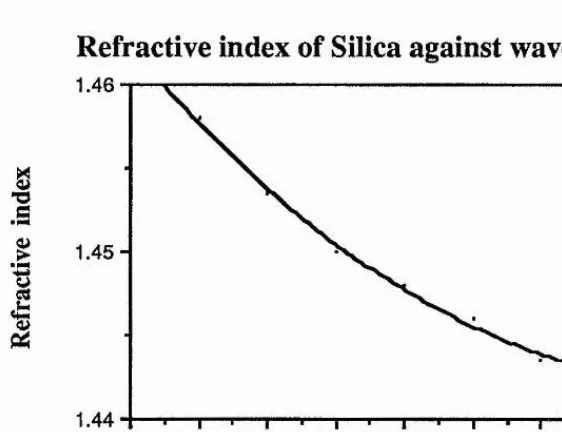
In the field of communications optical fibres are being developed for th eir large bandw idths. A figure of m erit for an optical fibre is usually given as a length-bandw idth product and is m easured in m egahertz or gigahertz per kilometer. The bandw idth of an optical fibre is related to the dispersion effects in the fibre. From bandwidth theory the bandw idth ôv is approximately 1/ôt where ôt is the pulse w idth of the signal. Any broadening of a pulse by an optical fibre decreases the available bandwidth. Pulse broadening by an optical fibre is principally due to two processes, nam ely interm odal and m aterial dispersion. Interm odal dispersion arises from different modes having different propagation constants and hence traveling different optical paths, for example, the wavefront of a hybrid mode such as an EH mode follows a helical path about the optical axis as it propagates down the fibre. M aterial dispersion arises from the w avelength dependence of refractive index in silica. A graph of refractive index against wavelength is given in figure 2.4.

The combined effect of interm odal and m aterial dispersion on the bandwidth of a fibre is given by

B W I, = (2.3.1)

Bandwidths greater th an SGhz/Km are achievable for a singlemode fibre a t ISOOnm b u t even a m ultim ode step-index fibre has a bandw idth of around 200Mhz/Km which is far g reater th a n is achievable electrically w ithout significant attenuation losses. For example, for coaxial cable the attenuation losses sta rt to rise quickly above a few megahertz. Large bandwidths allow optical signals to be m odulated a t high fi'equencies. This is desirable in optical signal processing for several reasons. The higher the modulation frequency the faster data can be transfered. Many optical sources are pulsed so processing m ust be carried out w ithin the pulse duration. Many

rad a r system s operate a t gigahertz frequencies so fibre optical | processing of ra d a r signals req u ires g igahertz bandw idths.

Integrated optical devices such as acousto-optic spectrum analysers doppler shift light which can be heterodyned giving frequencies of the order of 100 MHz.

Pulse dispersion in a step-index optical fibre is group delay dispersion. Group delay may be w ritten

^ dp L dp . (2.3.2) ^ o = L - = 7 d T

V = k a n ^ ^ /2 A , (2 .3 .3 )

Differentiating we have

dv _ V dk k *

Then we may write for tq

(2.3.4)

We have an expression for p, from equation (2.2.1.3), which is

+ f , (2.3.6)

We w ant to elim inate y so we define a norm alised propagation constant b such th at

a »

V V V

Substituting for and v we have

= (l+2Ab), (2.3.8)

which may be approximated to

p^n^k (1+Ab), (2.3.9)

We now obtain an expression for the group delay dispersion which is

L d(n^k ) L v d(n^k Ab) . (2.3.10) c dk ^ c k dv

The group delay dispersion can be seen to separate into two components,

Tg = Tc+ t^ , (2.3.11)

where xc is the group delay due to chromatic or m aterial dispersion and depends on the linewidth of the source and tm is the group delay

due to the difference in optical path length for each mode of the fibre.

2.3.1 Material Dispersion

We shall now consider the m aterial dispersion in a step-index optical fibre. From equations (2.3.10) and (2.3.11) the group delay of a mode due to m aterial dispersion is given by

As k = CO (|ie)i/2 we have

X = L d(n^co) , (2.3.1.2)

dco

expanded this becomes

T = i:(n + c Æ ) . _{c c} (2.3.1.3)

dco

We define a group refractive index Nq given by

dn . (2.3.1.4)

N,-, = n + CO—

° dco

. dn . (2.3.1.5)

0

The relative bandw idth of a source is ^X/Xq where ÔA, is a spread of w avelengths X2- X1 around Xq. If the energy propagates through a fibre of length L, then the spread of arrival times due to the different wavelengths is

- (2.3.1.6)

or

LdN_

dT = --- 2 ax. (2.3.1.7) c dX

Now we can substitute for Nq to obtain the delay corresponding to the

m aterial dispersion in a step-index optical fibre. This is given by

L

dx^ = - - 2 L dX, (2.3.1.8) dA,^

or, if we include the relative bandwidth of the source, we get

T AX d^n. . (2.3.1.9)

dx = — (— ) D where D

=---° c X ®d>.2

0

A graph of D against wavelength is given in figure 2.5.

2.3.2 Intennodal Dispersion

We now w ant to consider the interm odal dispersion in a step-index multimode optical fibre. From equations (2.3.10) and (2.3.11) we have

_ L V dCn^kAb) . (23.2,1) . c k dv

We also have an expression for v, equation (2.3.3), which is approxim ately

= kaiij«y2A = k a . (2.3.2.2)

Substituting v into (2.3.2.1) allows the interm odal dispersion to be expressed as

(2.3.2.3) ^ 0 2 dv

The derivative may be shown to be given approximately by 1-x/v [2.10]. Thus, the following useful form for the interm odal dispersion is

(" r (2.3.2.4)

For highly multimode fibres w ith large v, this expression becomes approxim ately equal to the geometric result obtained by considering the optical path difference between the axial and critical ray, figure 2.6. By considering the path difference between the axial and critical ray we have

= — [ Lmax - L ]. (2.3.2.S)

= !)]• (2.3.2.6)

” Cos

e

W hen the critical angle is expressed in term s of refractive indices we have

L L

“ “ ^1 ~ • (2.3.2.7)

2.4 Phase Dispersion in a step-index fibre.

An amplitude splitting optical fibre in terferom eter allows the correlation of an EM wave w ith a delayed version of itself. In free space the delay between the two waves is simply L/c where L is the path difference. However, in a dispersive medium the delay between the two waves becomes L / v p , where v^ is the phase velocity of the wave in the medium. Phase velocity is given by

V , (2.4.1)

' P

where p is the wavenum ber of the light in the m edium and co the angular frequency which is fixed. The wavenumber of the light in the medium depends on the boundary conditions imposed on it. In a step- index m ultimode fibre illum inated by a monochromatic source each mode has a different wavenumber.

From equation (2.2.1.2) we have

(2.4.2)

where = n^k (n^ is the refractive index of the medium and k is the free space wavenumber) and k^ is the wavenumber a t cut-off. From section 2.2.2, the cut-off w avelength for a step-index fibre m ay be determined by the root of the equation

W = 0 , (2.4.3)

W = 0 . (2.4.4)

The phase velocity of a given mode may then be w ritten as

The expression for the v num ber of a mode at cut-off is

Vg = k^a (n^ - n^), (2.4.6)

w here kc is the cut-off wavenum ber. By substituting (2.4.6) into (2.4.5) we have for the phase velocity

^ , • (2.4.7)

a (n^-n^)

For a mode whose v num ber a t cut-off is v^ the phase delay in a fibre of length L is

9t = - / (n k ) ^ . ( Z 4 = ^ ) \ (2.4.8)

o> \ l a (n^-np

From equation (2.4.8) we see that, for a multimode optical fibre, the phase delay decreases as v^ ^ increases. Now , substituting for

CO (= ck ) a n d w it h e q u a t io n (2.2.1.18), w h ic h i s

V = ka(ni2-n22)i^, (2.2.1.18)

= , (2-4.9)

or

a

t = - , / < -

.

(2.4.10)

We know that the wavenumber p in the fibre lies between two values as follows

n^k % p < rijk. (2.4.11)

Rearranging equation (2.4.2) we see th at

k^ = k^ - (2.4.12)

The maximum value of k^ occurs for p = Ugk and the m inim um value of kg occurs for p = n^k. The minimum value of the phase delay using (2.4.10) is therefore ngk and the maximum value of phase delay is njk. The m aximum difference in the phase delay betw een the modes of a fibre, At, may be w ritten

At = -^nj^-112) . (2.4.13)

■2«4iX..QpMcàl F a #

W hen considering the optical p ath length (OPL) of a fibre for inclusion in an interferom eter, or any situation where the OPL is im portant, then it is the phase dispersion which m ust be taken into account. Phase velocity has been discussed in section 2.4 and has been defined as

V =-^2- , (2.4.1)

B *^mn

where is the wavenumber of the wave propagating in the mn^^ mode. The OPL between two points A and B is defined as the velocity of light in a vacuum, c, m ultiplied by the time taken to travel from A to B, 6T. Thus, we can write

OPL = c6T . (2.4.1.1)

We m ay also write th a t the time taken for light to travel from A to B, in the mnth mode, is the distance, L, divided by the velocity in the medium. We have

8T = L = — _ (2.4.1.2) V p CO

The OPL of the mn^^ mode is, therefore,

cLp_^

O P L _ = _{mn ^}22Ü . (2.4.1.3) CO

In free space, we have c = co / k, so equation (2.4.1.3) becomes

LB

OPLmn = n f ^ - <2A1.4)

In a dispersive medium of refractive index n, we have

y ___2_ . (2.4.1.5)

n(^)

Thus, a different expression for the OPL is

OPL = c = Ln(X). (2.4.1.6)

Comparing (2.4.1.4) with (2.4.1.6) we see th at a mode of wavenumber Pmn an effective refractive index, n^^, given by

= • (2.4.1.7)

Following the working of section (2.4) on phase velocity we have th at the optical path length of the mn^^ mode is given by

OPL^ = k / n? - , (2.4.1.8) V

and the maximum optical path difference between the modes, for a fibre of length L, is given by

A(OPL) SL(nj-ii2). (2.4.1.9)

2.5 Interference

M any pre-detector signal processing techniques produce interference p a ttern s. The ap p aren t positions of two sources and th e ir wavelength determ ines the fringe geometry, th a t is, w hether the fringes are linear or circular and the fringe separation.

W hen two or more waves overlap they interfere in accordance with the principle of superposition to produce a series of bright and dark regions where the waves reinforce or cancel each other. By the principle of superposition the electric field at a given point, P, is the vector sum of the separate electric fields at th at point. We can write

Ep = Ej + + (2.5.1)

As the phase of an optical wave is repeated at about Hz, a detector m easures the time average value of power or intensity.

I = < l E p l ^ > = + (2.5.2)

If we consider and E2 to be two linearly polarised plane waves m propagating in directions r^ and rg with wavenumbers k^ and kg and | frequency co, then the two waves may be represented by

E^ = EqjCos (cot -kj.tj+(|)p , (2.5.3)

and

E2 = Eg^Cos (cot - . (2.5.4)

Expanding equation (2.5.2), we have

I = < Ie/ > + <IEjl^> + 2< lEjEjl > . (2.5.5)

The third term on the right hand side is the interference term . Substituting for and Eg , we have for the third term

E^.E^ = Eqj.Eq^Cos (cot-k^,rj+<()pCos(cot-k2.r2+(|)2), (2.5.6)

or

Ej.E2 = 1/2 E01.E02C0S (6), (2.5.7)

w here

6= ki.ri + (j)i - kg.rg - <(>2. (2.5.8)

The intensity a t P will be a maximum when Cos 6 = 1, th at is, when the phase difference between the beams is 2m7i, where m is a positive or negative integer. This corresponds to the condition for constructive interference. The intensity a t P will be a m inim um when Cos 6 = -1. T hat is, when the phase difference between the beam s is (2m+l)%, where m is a positive or negative integer. T his corresponds to the condition for destructive interference.

If E j and Eg are parallel then we m ay write

I = I, + 12 + 2,yïjï^Cos (S). (2.5.9)

If II and Ig are of equal intensity we have

where Ïq is the m axim um intensity. The m any ways of producing interference can be divided into three groups, polarisation splitting, wavefront splitting and amplitude splitting. Polarisation splitting will not be considered. W avefront splitting implies th a t different portions of a single w avefront are used to produce two or more sources which then interfere. Amplitude splitting implies th a t a single wavefront is divided into several identical wavefronts which travel different paths before they overlap.

2.5.1 Wavefix>ntsplittln£f interferometers

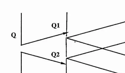
An example of a wavefront splitting interferometer is th a t used in the Young's interference experiment, figure 2.7.

Light is incident on a single pinhole Q and then on a pair of pinholes Qi and Qg. The two spherical waves emerging from Qi and Qg fall onto a screen and interfere in the region where the waves overlap. If the amplitudes of the waves are the same and the two slits are of equal width and very close together, then the intensity a t a point P on the screen is given by equation (2.5.10), which is

I = 4IgCos^A . (2.5.10)

At P, the waves from Qi and Qg have traveled distances Q^P and QgP. The phase difference between them at P is ô where

5 = — (Q,P-Q,P). (2.5.1.1)

X

It is assumed th a t the waves have the same phase a t the two pinholes. The path difference QgP - Q^P is the distance QgR in figure

2,8. When the distance between the pinholes is small compared with the distance from the pinholes to the screen we can m ake the approxim ation

Q.R . (2.5.1.2)

Sin 0 = —-— _d

In this case, the phase difference between beams is given by

5 = _ ( d Si n e ) . (2.5.1.3)

X

For I to be a maximum, th a t is, for a bright interference fringe, 6 = 2m7c as before. Thus, for the m^h bright fringe, we have

2tc

2mjc= — dSinO, (2.5.1.4) X.

or

= d Sin 0 . (2.5.1.5)

We then make the further approximation th at the angle between the optical axis and the light which travels to the m^h fringe is given by

Sin 0 = ^ ' (2.5.1.6)

w here r^ is the position of the m^b bright fringe. From equations (2.5.1.5) and (2.5.1.6) , we have th a t the position of the mth bright fringe is given by

m X D . (2.5.1.7)

For I to be a minimum, or a dark fringe we require 6 = (2m+l)%. Thus, for the m^b dark fiinge we have

(2m+l)7C = . ^ d S i n e , (2.5.1.8)

X

or

(m + 1/2)X = d Sin 0 . (2.5.1.9)

Using equation (2.5.1.6) as before we have

(m+l/2)?i = • (2.5.1.10)

This m ay be rearranged to give, for the position of the mth dark fringe, th at

(m+1/2) ID . (2.5.1.11)

2.5.2 Amplitude splitting interferometers

As an example of an amplitude splitting interferometer we consider the Michelson interferometer, figure 2.9. A wave from a source, S, is incident on the beamsplitter, B. The wave is split into two waves of equal amplitude. The first p a rt travels to mirror m j where it is reflected and the second p a rt travels to mirror m2 where it is also

reflected. The waves are recombined a t B and propagate to a screen where circular interference fringes may be observed.

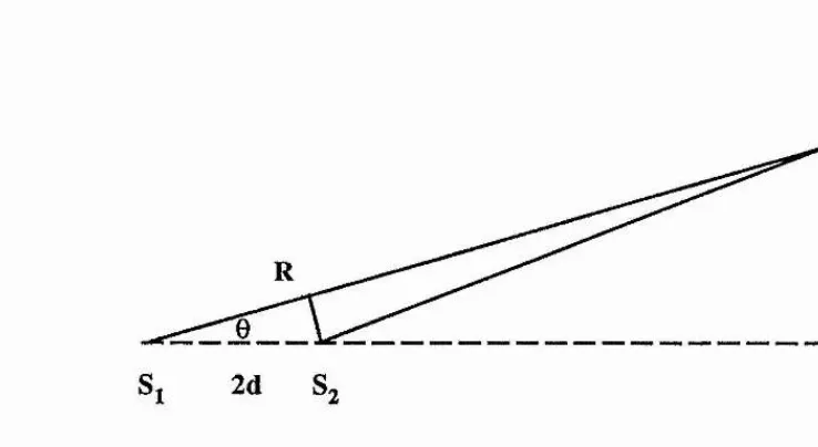
The two mirrors produce two apparent sources a distance 2d apart where d is the p ath difference in the arms of the interferometer, figure 2.10. The distance the waves appear to have traveled to a point

p on the screen is S^P and S2P. The phase difference between the

beams a t P is 6 where

ô = ^ ( S j P - S 2 P ) . (2.5.2.1)

A.

This distance can be seen to be S^R, so we can write

2tc

8 = — ( 2 d C o s 0 ) . (2.5.2.2)

%

The intensity distribution across the rings is given by equation (2.5.10), written

I = 4IgCos^A . (2.5.10)

For the waves to interfere constructively we require 6=2m7c where m

is an integer. So, for a bright ring, we have

mX = 2dCos 0. (2.5.2.3)

For the waves to interfere destructively we require ô=(2m+l)7i. So, for a dark ring, we have

(m+1/2)^ = d Cos e . (2.5.2.4)

The radius of the rings depends on the separation of the mirrors M i and M2. For a ring of order m the angle of the ring from S% is given

h y

^ ^ mX. (2.S.2.5)

As the p ath difference, d, is increased the radius of the mth fringe decreases. As d becomes smaller, the two sources S i and S2 become

coincident and the central fringe expands to fill the entire field of view.

2.g ÇçheygitçgTbeçry

Coherence is a measure of the degree of correlation of the phases of different waves a t different times or locations. The degree of correlation m ay be investigated using an interferometer. If the correlation is between two waves separated in time we measure the temporal coherence of the light. If the correlation is betw een two waves originating from different points in space measure the spatial coherence of the light.

A source has a characteristic frequency spread or bandw idth dv. From the bandwidth theorem we have

dt a — , (2.6.1)

dv

where dt is the coherence time of the source. This corresponds to the time over which a wave packet from the source has a predictable phase and since a wave travels a distance cdt in this coherence time, cdt is the coherence length, Lc. We have

= c dt = — . (2.6.2) dv

The bandw idth ôv is related to the linewidth 6X. Differentiating v = c /

X we obtain

dv = — dA,. (2.6.3)

By substituting (2.6.3) into (2.6.2) we may express the coherence length in terms of the central wavelength and linewidth of a source. Thus, we have

L = 21 . (2.6.4)

When a spatially incoherent source illuminates a plane, we m ay define a coherence w idth which is equal to the maximum separation of two points which will produce interference fringes.

Consider the geometry of figure 2.11. Two sources Si and Sg each illuminate a plane containing two slits as w ith a Young's slits experiment. Both sources produce interference patterns in a second plane. The interference patterns are m utually incoherent. As Sg is in a different position to Si the phases of the interference patterns are slightly different. If the separation of the slits. Pi and P g , is sufficient so th at

QPj = - S^Pj = i x , (2.6.5)

then the bright fringes due to Si will be superimposed on the dark fringes due to S g , and visa versa, so no fringes will be seen. The

minim um separation of P i and Pg , before this occurs, defines the

coherence width. The path difference QPg is given by

QPg = d^ Sin 0 , (2.6.6)

where dc is the separation of the slits, or the coherence width. The angle 0 may be expressed as

d /2 d.

Sin 0 = . (2.6.7)

As D = D1 + D2 we have

1 _ .

S i n 0 = ^ ( d g + y ) . (2.6.8)

From equations (2.6.6) and (2.6.8), the path difference QPg is given approximately by

d d

Q P g = . ( 2 .6 .9 )

Thus, no interference will be seen w hen the two sources are separated by a distance dg, where

d^= j y . (2.6.10)

c

If th e two point sources a distance dg apart, are replaced by an extended source of size dg th en no interference fringes will be seen. The area of the extended source, Ag, may be related to a coherence area, A^. We can write

A S — . (2.6.11)

2.6.1 The Analytic Signal

The analytic signal is of use in discussing a linear optical system and will be used in the following sections to define the coherence of two waves which are allowed to interfere. A linear system is one in which several impulses cause a response which is the sum of the individual responses.

represented by the real function E (t) which is a real disturbance and may be expressed in the form

= J A(v) Cos [ (})(v) ~ 27üvt ] dv, (2.6.1.1)

where A(v) is the amplitude and (j)(v) the phase. A second real function E (t) may be defined by replacing (})(v) by (j)(v) - %/2. We then have

E®\t) = IA(v) Sin [ (|)(v) - 2 n vt ] dv. (2.6.1.2)

These two functions m ay be combined in a single exponential function E(t) which is w ritten

E(t) = E^'^t) + i E®(t) = Ja(v) e ^ dv. (2.6.1.3)

If A(v) is the Fourier transform of E^^^(t), then since E^^^(t) is real we have

A(-v) = A*(v) . (2.6.1.4)

This is because all the inform ation about E^^) (t) is contained in the positive frequency region of the spectrum. Equation (2.6.1.3) can be w ritten

00

E(t) = 2Ja(v) e^"^'dv. (2.6.1.5)

The function E(t) is known as the analytic signal. If the operations carried out upon E(^)(t) are linear, then the more convenient function E(t) can be used in the analysis and E^*’^(t) obtained at the end. If the amplitude of the components of the spectrum is significant only over a region 6v which is sm all compared w ith the mean frequency v, then we write the analytic signal in the form

E(t) = Eg(t) e‘ ( (2.6.1.6) The real part is then given by

E®(t) = Ep(t) Cos [ <|)(t) - 2itvt ]. (2.6.1.7)

2.6.2 Coherence as dofinotl hv correlation integrals.

We can use the analytic signal to define the coherence of an electromagnetic field in terms of a correlation over the field. If E(r,t) is the field a t a given point in space and time and if the field is observed for a time x which is large compared with its mean period

1/v then the auto-correlation, rjj(r,t), or the self coherence function of the field may be expressed as

+x

r (r,t) = lim x->c>o_L fE(r,t) E*(r,t) d t. (2.6.2.1) "T .

The temporal coherence of the field may be expressed as +x

r , , (r.t+T) = — fE(r,t) E*(r,t+T) d t, (2.6.2.2) 2 f_{- X}

-PC

= —JE(r,t) E*(r+dr,t) dt. (2.6.2.3)

2x_{- X}

These definitions will be used in the following sections.

2.6,3 Temporal coherence

The device m ost commonly used to measure temporal coherence is the M ichelson interferometer. This interferometer has two air paths, one of which is used to alter the delay between the two waves. Light from a scene is introduced to the interferometer. The light is divided into two waves of equal amplitude by the beamsplitter, B. One wave is reflected from mirror ml and other is reflected from mirror

m2. The two w aves are recombined a t B and th e resu ltin g

interference measured a t the output plane P, as was shown in figure 2.9.

The light introduced to the interferometer is represented by E(x,y;t) where x and y are the norm al space coordinates and t is time. If E i(x ,y ;ti) represents the amplitude of the wave which has been reflected from mj and Eg(x,y;t2) represents the amplitude of the

wave reflected from m2 then the complex field at P is

Ep(x,y;ti,t2) = Ei(x,y;ti) + E2(x,y;t2). (2.6.3.1)

The intensity measured by a detector at P is the time averaged square modulus of the amplitude. We have

Ip(x,y;ti,t2) = < I Ep(x,y;ti,t2)|2>, (2.6.3.2)

where <> implies a time average and I I means modulus. Expanding the right hand side of this equation gives us four terms , which are

I(x,y,t^,y = < iEj(x,y,tj)l^ + lE^Cx^y^t^)!^ + E^*(x,y,t^)E2(x,y,y +

E j ( x , y , t j ) E 2 * ( x , y , y > . ( 2 . 6 . 3 3 )

An asterisk denotes complex the conjugate. If the statistics of the radiation are assumed to be stationary, we can w rite t% = t , and tg = t + X . Then we have

I(x,y,x) = < I E^(x,y,t) 1^ + I E^(x,y,t+x) P + E^*(x,y,t)E^(x,y,t+x) + E^(x,y,t)Ey(x,y,t+x) > . (2.6.3.4) The first and second terms on the right hand side of equation (2.6.3.4) represent the intensities measured by the detector if either mirror were the only one present. They provide a constant background level and may be w ritten as

I E^(x,y,t) 1^ = Ij(x,y,t) , (2.6.3.5) and

I E^(x,y,t+x) ^ - yx,y,t+ x). (2.6.3.6) The third and fourth terms can be replaced by

< Ej(x,y,t) E^*(x,y,t+X) > = T^^(x), (2.6.3.7) and

< Ej*(x,y,t) E^ (x,y,t+x) > = F^^*(x), (2.6.3.S)

where F(x) is the temporal m utual coherence function. The function represents the cross correlation of fields E% and E2 a t the same point

bu t w ith time delay x between them. Substituting equations (2.6.3.5), to (2.6.3.S) into (2.6.S.4) we have

As ri2('c) represents an auto-correlation of a wave w ith a delayed version of itself we m ay apply the auto-correlation, or W iener- Khinchin, theorem . This states th a t the Fourier transform of the auto-correlation of function T1 2W is the power spectrum, Fi2(v), of

th a t function. We also note th at the position coordinates are the same and so we drop the position dependence. We can write

= J

and

so equation (2.6.3.13) becomes

I(t) = I^(t) + I^d+T ) + 2\ F^^(x) I Cos (2jw^t + 4>^(x)), (2.6.3.15)

32

r^^*(x) = J

0

Since the power spectrum m ust be real, we have F i2(v) = F i2*(v). (2.6.3.12)

The source is considered to be quasi-monochromatic, so dv / V o« 1

where dv is the spectral w idth and Vq is the mean frequency. Then (2.6.3.9) becomes

00

I(X) = Ij(t) + y t + x ) + J 2 I Tj^(v) I Cos (2mVgX + (t)(x) ) d v . (2.6.3.13)

0

We can write

ri^(T) = |F^^(x)|Cos(27UV^t + <|)^(x)), (2.6.3.14) |

where F12W is the Fourier transform of the frequency distribution of

the source. The cosine term can be seen to give information about the temporal m utual coherence function, F(x) and through this F(v).

We can define a norm alised m utual coherence function which is F, fx)

y . M ---12--- . (2.6.3.16)

(I,(t)y t-K ))i'2 w ritten

Using equations (2.6.3.15) and (2.6.3.16), we have

I(x) = Y t) 4- I^(t4-x) + 2 (I^(t)I^(t+x))^/^ I y^^(x) I Cos (270'^t+())^(x)) .

(2.6.3.17) If the waves are of equal intensity, we have I%=l2=I and (2.6.3.17)

becomes

I(x) = 21(1 + 1 Y^^(x) I Cos (27cv^t + 4)^(x)) ). (2.6.3.18) This is the relationship for the output of a F ourier transform

spectrometer. As a measurable quantity we use Michelsons visibility V defined by

v = . (2.6.3.19)

max min

The maximum value of I(x) occurs when we have

Cos(2jwot+<l)r(x)) = 1 , (2.6.3.20) and the minimum value when we have

Cos(27cvot+<t>r(x)) = -1. (2.6.3.21)