CMB constraints on cosmic strings and superstrings

Tom Charnock,∗ _{Anastasios Avgoustidis,}† _{Edmund J. Copeland,}‡ _{and Adam Moss}§ Centre for Astronomy & Particle Theory, University of Nottingham,

University Park, Nottingham, NG7 2RD, U.K.

We present the first complete MCMC analysis of cosmological models with evolving cosmic (super)string networks, using the Unconnected Segment Model in the unequal-time correlator for-malism. For ordinary cosmic string networks, we derive joint constraints on ΛCDM and string network parameters, namely the string tensionGµ, the loop-chopping efficiencycr and the string wigglinessα. For cosmic superstrings, we obtain joint constraints on the fundamental string tension GµF, the string couplinggs, the self-interaction coefficientcs, and the volume of compact extra di-mensionsw. This constitutes the most comprehensive CMB analysis of ΛCDM cosmology + strings to date. For ordinary cosmic string networks our updated constraint on the string tension, obtained using Planck2015 temperature and polarisation data, isGµ <1.1×10−7 in relativistic units, while for cosmic superstrings our constraint on the fundamental string tension after marginalising overgs, csandwisGµF<2.8×10−8.

I. INTRODUCTION

Cosmic strings are line-like concentrations of energy that can arise as topological defects in theories of the early Universe [1–5]. In particular, they form natu-rally in models of hybrid inflation [6–12] in which the inflationary phase ends with a second-order phase-transition [7, 13–15]. Although they were originally considered as an alternative candidate for providing the seeds for structure formation in the Universe [16–

19], it is now understood that they cannot give rise to the observed acoustic peak structure in the power spectrum [20–24], but can play a subdominant role. There are a wide range of potential observational sig-natures of cosmic strings, for example line-like discon-tinuities in the cosmic microwave background (CMB) temperature anisotropy via the Kaiser-Stebbins ef-fect [25,26]. Thus, strings provide a powerful tool for testing theories of the early Universe. Observations have strongly constrained the contribution of cosmic strings to the total CMB anisotropy [20,27–32]. Cur-rent data place a 2σ upper bound on the string ten-sion ofGµ <1.3×10−7 for Nambu-Goto strings [33] or Gµ < 2.7×10−7 for Abelian-Higgs strings [34], which corresponds to ∼1% of the total temperature anisotropy at`= 10. Gis the gravitational constant,

µis the tension of the string andc= 1 in relativistic units. Although this may seem insignificant, there is still constraining power left in the data since strings generate specific signatures in the primordial B-mode polarisation spectrum [27, 35–40], which can now be analysed with the Planck2015 polarisation [41] and joint BICEP2 data [42].

Going beyond the simplest cosmic string models, complex networks of multiple types of interacting su-perstrings, each with a different tension, can also be considered. Notably, interacting networks of fun-damental F-strings, one dimensional D-branes (strings) and bound (FD) states between F- and

D-∗_{[email protected]} †_{[email protected]} ‡_{[email protected]}

§_{[email protected]}

strings, collectively referred to as cosmic superstrings, arise naturally in string theoretic inflation [7,43,44]. These networks are notably different to their sim-pler, single-type string counterparts since the differ-ent string types have intercommutation probabilities that are not necessarily unity [44–50]. The interac-tions among different string types are also much more complex, as colliding strings can zip together or unzip, producing heavier or lighter FD-string states carrying different charges. These features affect CMB signa-tures allowing us to obtain constraints on string the-ory parameters such as the string couplinggsand the

fundamental string tensionµF [51,52].

In this paper we use the Planck2015 public data [41] to perform the first full Markov chain Monte Carlo (MCMC) analysis of ΛCDM models with cosmic string or superstring networks. For “ordinary” cos-mic string networks we work in the unconnected seg-ment model (USM) framework and utilise our ana-lytic method [53] for fast computation of the string unequal-time correlator (UETC). This is used as a source to compute CMB anisotropies and hence ob-tain joint constraints on ΛCDM and the string net-work parameters, including the tensionGµ, the loop chopping efficiency cr and the wiggliness parameter

α. In the case of cosmic superstring networks we ex-tend our method to deal with multiple network com-ponents. The UETC approach is efficient, meaning we can compute the superstring spectrum in much less time than previous codes and obtain joint con-straints on the fundamental string tension GµF, the string coupling constantgs, the self-interaction

coeffi-cientcs, and the parameterwof [52], quantifying the

volume of compact extra dimensions.

In Sec. II we describe the UETC formalism ap-plied to evolving Nambu-Goto string networks. In Sec. III we summarise our modelling of cosmic su-perstrings and the adaptation of our UETC method to these multi-string component networks. In Sec.IV

II. UNEQUAL-TIME CORRELATOR

Unlike passive inflationary perturbations which are set as initial conditions, metric perturbations from cosmic string networks are actively sourced at all times. To compute the string spectra the compo-nents of the string network’s energy momentum ten-sor must be used as sources in the linearised Einstein-Boltzmann equations. The relevant quantity to cal-culate is the unequal-time correlator (UETC), whose dominant eigenmodes, found by diagonalising, can be used as source functions, each individual mode being coherent [19]. The UETC

hΘµν(k, τ)Θ∗αβ(k, τ

0_{)i ≡ Cµν,αβ(k, τ, τ}0_{) (2.1)} determines all the two-point correlation functions such as the CMB temperatureC`and matter power spectra

P(k), defined as in [54]. Θµν(k, τ) is the string energy-momentum tensor defined below.

A. String Energy-Momentum Tensor

Nambu-Goto strings are one-dimensional defects in the zero-width limit. They provide a good descrip-tion for long cosmic strings, whose correladescrip-tion length is many orders of magnitude larger than their width, at least away from string intersections. A string mov-ing in spacetime spans a two-dimensional surface, the worldsheetxµ_(σa_{), where the indicesµ= 0,1,2,3} la-bel spacetime coordinates and a = 0,1 are the in-dices of coordinates on the worldsheet [55, 56]. The worldsheet action is reparametrisation invariant and a gauge can be chosen by imposing two conditions on the spacetime coordinates xµ _{as functions of σ}a_{. In} an FRW background, a useful choice of gauge is such thatσ0_{=τ, the conformal time, andx}0_{·x˙ = 0, where} ˙ ≡∂/∂τ and 0 ≡∂/∂σ, relabelling σ1, which in this gauge is a spacelike worldsheet coordinate, as σ. In this gauge the Nambu-Goto string energy-momentum tensor is

Θµν(y) = √1 −g

Z dτ dσ

U

r

−x

02

˙ x2x˙

µ_x˙ν_−T

r

−x˙

2

x02x

0µ_x0ν

δ(4)(y−x(τ, σ)). (2.2)

Here, U is the string energy per unit length andT is the string tension. For Nambu-Goto strings on arbi-trarily small scales, Lorentz invariance requires that

T =U =µ. However, if we coarse-grain the string, then the integrated effect of small-scale structure is to make the effective tension smaller than the energy density. We can then include the effect of small-scale wiggles on the string via a “string wiggliness” param-eterα, such that

U =αµandT = µ

α, (2.3)

satisfyingU T=µ2_.

The Fourier transform of the 00-component of the energy-momentum tensor of a representative string segment in a network is

Θ00(τ,k, χ) = µα

√ 1−v2

sin(k·Xˆξτ /2) k·Xˆ/2

×cosk·x0+k·X˙ˆvτ

, (2.4)

wherevandξare the string network velocity and co-moving correlation length, defined in Sec.II Bbelow, and x0 is the position of the string endpoint. The

string segment is parametrised by

x(σ, τ) =x0+σXˆ +vτX˙ˆ, (2.5)

with the string orientations and velocity orientations

ˆ X=





sinθcosφ

sinθsinφ

cosθ 

, (2.6)

˙ˆ X=





cosθcosφcosψ−sinφsinψ

cosθsinφcosψ+ cosφsinψ

−sinθcosψ



. (2.7)

˙ˆ

X is transverse to ˆX such that ˆX·X˙ˆ = 0. Note that the position of the string endpoint appears only through a phase in the cosine factor in equation (2.4), which we will denote asχ≡k·x0. The other

compo-nents of the string energy-momentum tensor are given by

Θij =

v2X˙ˆiX˙ˆj− 1−v2

α2 XˆiXˆj

Θ00, (2.8)

with i, j = 1,2,3. Choosing coordinates so that k lies along the ˆk3 axis, the scalar, vector and tensor anisotropic stresses are given by

ΘS= 1

2(2Θ33−Θ11−Θ22), (2.9)

ΘV= Θ13, (2.10)

ΘT= Θ12. (2.11)

B. Velocity Dependent One-Scale Model

L, and the average velocityv, of string segments in the network [57]. The correlation lengthLis the average length of string segments which, for scaling networks (that have a random walk structure), is also equal to the average string separation. The network veloc-ityv, is the root-mean-square (RMS) velocity of these correlation-length-sized string segments averaged over all (shorter) length scales. The macroscopic evolution equations for these network parameters can be derived from the Nambu-Goto action by applying a statistical averaging procedure over the string worldsheet [58–

60]. Expressed in terms of the physical time t they read:

˙

L= (1 +v2)La˙

a+

crv

2 , (2.12)

˙

v= (1−v2) _˜

k L−2v

˙

a a

, (2.13)

wherea(t) is the scale factor, ˙a(t)/a(t) is the Hubble function and from now on ˙ ≡ d/dt, unlike in equa-tion (2.2). The loop chopping efficiency parametercr, quantifies the energy loss due to loop production and ˜k

provides a phenomenological description of the small-scale structure on the string, which, for relativistic strings, is given by

˜

k=2 √

2

π

1−8v6

1 + 8v6

. (2.14)

The correlation length can be written in comoving units as ξτ =L/a. The VOS equations in comoving units are

ξ0= 1

τ

v2ξτa 0

a −ξ+ crv

2

, (2.15)

v0= (1−v2) _˜

k ξτ −2v

a0 a

, (2.16)

where now 0 ≡ d/dτ unlike in equation (2.2). For fixed expansion rate the scaling solutions, found by the requirementξ0= 0 and v0= 0, read

ξ= s

˜

k(˜k+cr)(1−β)

4β , (2.17)

v= s

˜

k(1−β)

β(˜k+cr)

, (2.18)

whereβis the physical time FRW expansion exponent

a(t)∝tβ _{and is equal to 1/2 and 2/3 in the radiation} and matter eras respectively. Note in the scaling so-lutions of (2.18) the implicit velocity dependence of ˜

k through equation (2.14). Earlier implementations of the cosmic defect CMB codeCMBACT[61] used two sets of values for the loop chopping efficiency and the parameter ˜k in the scaling solutions (2.18) for the radiation and matter eras. These values were then interpolated between for the transition between the radiation and matter eras. However, in the latest im-plementation of the VOS equations in CMBACT4 [62], the velocity dependence of ˜kis explicitly used and the loop chopping efficiency is kept constant throughout

0.0

0.1

0.2

0.3

0.4

10

₁₀

₁₀

₁₀

₁₀

₁₀

0.5

0.6

0.7

10

10

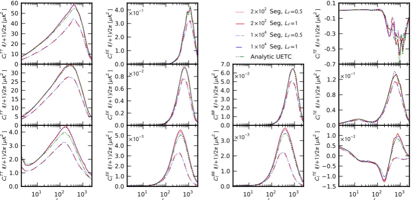
10

FIG. 1. The evolution of the velocityv, and correlation lengthξ, for a range ofcr= [10−2,1.0]. The black dot-dot-dash line indicates the correlations lengths and velocities obtained when cr = 0.23. The greener area (lighter in black and white) of the plot indicates larger values of cr whilst the more purple region (darker in black and white) shows smallercr.

both epochs [60]. Here, we also adopt this approach: at any particular τ, the values of ξ and v found us-ing the VOS equations (2.15-2.16) are used for cal-culating the UETC, keeping cr constant throughout

and explicitly accounting for the velocity dependence (2.14) of ˜k. In earlier versions of CMBACT the wiggli-nessα, was also an evolving parameter, but it is now kept constant in CMBACT4, which is the approach we take here. The evolution of the network parameters can be seen for a range of cr in Fig. 1 showing that

a wide range of correlation lengths and velocities are available. Detailed comparison of the VOS model with Nambu-Goto simulations of ordinary string networks (i.e. single string type with unit intercommuting prob-ability [63]) determine the loop chopping efficiency to cr = 0.23±0.04 [60], corresponding to the black dot-dot-dashed curves in Fig. 1. Models of cosmic superstrings generally have suppressed intercommu-tation probabilities [45–48], which effectively reduces

cr and so they correspond to the purple region in the

figure. Such networks have relativistic RMS velocities

v∼1/√2 and correlation lengths much smaller than the horizon, corresponding to a much higher string number density compared to ordinary string networks. However, they also have smaller string tension so their overall effect on the CMB can be small, consistent with the data.

veloc-ity distribution with larger velocities at short scales, implying that the RMS velocity is dominated by rel-ativistic speeds at short distances. On length scales of order the correlation length, coherent velocities as low as vcoh '0.2 have been reported [64–67]. Other

network velocity measures (again containing informa-tion from a range of length scales) in both Nambu-Goto and Abelian-Higgs string simulations also tend to be lower than the VOS RMS velocity, with veloc-ities in the Abelian-Higgs model vAH ' 0.5, signif-icanlty slower than in Nambu-Goto simulations [68–

70]. For further discussion about the impact of string velocities on the UETC and the string power spectrum see the end of Sec.II F.

C. Unconnected Segment Model

Simulations of evolving string networks are numer-ically very expensive. Strings decay as 1/(ξτ)3_,

even-tually reaching a scaling solution (ξ= constant) with a number density of tens to hundreds of strings per horizon volume. At early times, the box contains a huge number of strings whose dynamics and inter-actions have to be tracked at each time step. The unconnected segment model (USM) [21,61] dramati-cally reduces the required computational resources by approximating the string network as a collection of correlation-length-sized segments, with the time evo-lution of the correlation length and segment veloc-ity described by the VOS equations. Moreover, the model consolidates these string segments by collect-ing all strcollect-ings that decay between any two times, and so fewer strings need to be tracked. The number of strings that decay between any two conformal times in a volumeV, is

Nd(τi) =V[n(τi−1)−n(τi)], (2.19) wheren(τ) is the number density of strings at confor-mal timeτ, given by n(τ) =C(τ)/(ξτ)3. InCMBACT, the factor C(τ) is chosen so as to keep the number of strings at any time proportional to 1/(ξτ)3_{. The}

energy-momentum tensor for the string network is then given by the sum over the total number of con-solidated string segmentsK, with a factor accounting for string decay

Θµν = K

X

i=1 p

Nd(τi)ΘiµνT

off_{(τ, τ}

i, Lf). (2.20)

The string decay factorToff(τ, τi, Lf) is a function in-terpolating between 1 and 0 and is responsible for turning off the contribution of the ith _consolidated

segment after the time it has decayed. Its steepness is controlled by a string decay parameter 0< Lf ≤1,

as follows:

Toff(τ, τi, Lf) =

 



1 τ < Lfτi

1/2 + 1/4(y3_{−3y) L}

fτi< τ < τi

0 τi< τ

(2.21) where

y=2 ln(Lfτi/τ)

ln(Lf) −1. (2.22)

Thus, in the limit Lf → 1 the string decay fac-tor Toff(τ, τi, Lf) approaches a Heaviside function, sharply switching off the contribution of the ith

con-solidated segment to the network energy-momentum tensor for timesτ > τi.

TheLf Parameter

Since the number of consolidated segments also sets the number of decay epochs, a finite number of con-solidated segments leads to discrete steps in the num-ber density of strings. The string decay parameterLf

was introduced to allow a fraction of the consolidated strings to decay before the end of their respective de-cay epoch, thus making the number density evolution smoother. The function C(τ) was also introduced to ensure that the number of strings at any confor-mal timeτ is kept proportional to (ξτ)−3_{. However,}

one consequence of Lf <1 is that it is possible that

Lfτi+1< τi, meaning strings can start to decay earlier than their respective epoch and the number density is systematically lower.

In theCMBACT4implementation we have found that changing the number of consolidated segments from 200 to 10000 has very little impact on the string spec-tra, as shown in Fig. 2. However, the amplitude of theC` isdependent on the value ofLf. The change is scale dependent, but can be as much as 30%, for example near the peak of the scalar temperature sig-nal. Previous analyses which have used the results from CMBACT have overlooked this dependence. Al-though not entirely degenerate with the amplitude of

C`, which scales proportional to (Gµ)2, it will clearly have some affect on the inferred values of Gµ from the USM. We compare this to our approach in the following section.

Infinite Consolidated String Segments

We are able to accommodate a large number of seg-ments analytically. As discussed in [53], the scaling factor, that weights the UETC taking into account string decay, has a particularly simple form when the number of consolidated string segments tends to in-finity,Lf→1 andC(τ)→1. This is

f(τ1, τ2, ξ(τ1), ξ(τ2)) =

K

X

i=1

Nd(τi)Toff(τ1, τi, Lf)

×Toff(τ2, τi, Lf),

= (ξ(Max[τ1, τ2])Max[τ1, τ2])−3.

= f τMax, ξ(τMax) (2.23) An analytic expression for the scaling factor can also be found for arbitraryLf using the form ofToffquoted

101 ₁₀2 ₁₀3

0 10 20 30 4050 60

(+

)/

[

]

101 ₁₀2 ₁₀3

0.0 1.0 2.0 3.0 4.0

(+

)/

[

] _{× × Seg, = .}

× Seg, = × Seg, = . × Seg, = Analytic UETC

101 ₁₀2 ₁₀3

-0.7 -0.5 -0.3 -0.1 0.1

(+

)/

[

]

101 ₁₀2 ₁₀3

05 10 15 20 25 30

(+

)/

[

]

101 ₁₀2 ₁₀3

0.0 0.2 0.4 0.6 0.8

(+

)/

[

] _×

101 ₁₀2 ₁₀3

0.0 1.0 2.0 3.0 4.0 5.0 6.0 7.0

(+

)/

[

]

×

101 ₁₀2 ₁₀3

0.0 0.4 0.8 1.2

(+

)/

[

]

×

101 ₁₀2 ₁₀3

0.0 1.0 2.0 3.0 4.0

(+

)/

[

]

101 ₁₀2 ₁₀3

0.01.0 2.0 3.0 4.0 5.0

(+

)/

[

]

×

101 ₁₀2 ₁₀3

0.0 1.0 2.0 3.0

(+

)/

[

]

×

101 ₁₀2 ₁₀3

1.5 1.0 0.5 0.00.5 1.0

(+

)/

[

]

×

FIG. 2. C`obtained from the string realisation codeCMBACT4with 200 and 10000 consolidated string segments for 2000

string realisations between the red solid and dashed lines and blue dotted and dotted-segment lines respectively. The solid red and dotted blue lines at the top of each band indicate a value ofLf = 1 for 200 and 10000 segments, while the red dotted and blue dotted-segment lines showLf = 0.5. The top, middle and bottom rows show the scalar, vector and tensorC`modes respectively. The first column contains the temperature (TT)C`, the second column has the EE mode

contribution, BB modes are in the third and the TE cross-correlation in the final column. We also plot the corresponding spectra derived from our analytic USM method, shown in green dot-dot-dashed lines.

continuous limit in which the string number density is smooth. We have shown that the number density scales according to (ξτ)−3 _{with our approach. While}

infinite consolidated segments may seem unphysical, it is just a limit used to obtain the correct scaling rela-tion. We obtain very similar results toCMBACT4when using between 200 to 10000 segments with Lf = 1. The question of whether the observed resulting mod-ification of scaling from early string decay obtained whenLf <1 is physical or not requires investigation.

Since we takEC(τ) = 1 we avoid considering different scaling behaviour. Ultimately, the USM is a simplified model which aims to match the UETC from simula-tions by adjusting the network parameters. Overall it has been shown to match Nambu-Goto simulations well [71]. However, due to the correlation between the inferred values forGµfor a givenLf, this issue should

be considered more closely.

Since the number density scales according to (ξτ)−3

using our approach, we believe this to be reasonable and will adopt this for the comparison to data.

D. Analytic Calculation of the Unequal-Time Correlator

The UETC can be computed analytically [53] by integrating over all string configurations (orientations and positions) in the network. For the two point cor-relator between Θ(τ1,k1, χ1) and Θ(τ2,k2, χ2) trans-lational invariance implies k1 = −k2 = k and so χ1 = −χ2 = χ. Considering that, due to equations

(2.4) and (2.8), Θ(τ,k, χ) is a symmetric function of kthe integral is

hΘ(τ1,k)Θ(τ2,k)i=2f(τMax, ξ(τMax)) 16π3

Z 2π

0 dφ

Z 2π

0 dψ

Z π

0

sinθdθ Z 2π

0

dχΘ(τ1,k, χ)Θ(τ2,k, χ). (2.24)

Without loss of generalitykcan be chosen to lie along thek3-axis, such thatk=kˆk3. Θ here represents each

of Θ00, ΘS, ΘVand ΘTof equations (2.9-2.11). Theφ, ψandχintegrals can be done analytically in this case

leaving only theθintegral in terms of Bessel functions. The UETC can then be written as the sum over six integral identities

hΘ(τ1, k)Θ(τ2, k)i=

f(τMax, ξ(τMax))µ2 k2p

1−v(τ1)2p

1−v(τ2)2 6 X

i=1

Ai[Ii(x−, %)−Ii(x+, %)], (2.25)

where%=k|v(τ1)τ1−v(τ2)τ2|andx±= (x1±x2)/2

with x1,2 = kξ(τ1,2)τ1,2. Here x1,2 means x1 or x2

of [53] in that ξ and v are now functions of τ in-stead of being kept constant. This means that the expressions of the amplitudes Ai, presented in Ta-ble II, are now time-dependent. The integral identi-ties (shown in TableI) remain the same. It should be noted that I1(x, %) andI4(x, %) diverge but the com-binationI1,4(x−, %)−I1,4(x+, %) is regular and, in the

limit where x1,2 x2,1, has an analytic

approxima-tion given by

I1(x−, %)−I1(x+, %) = πx1,2

2 J0(%), (2.26)

I4(x−, %)−I4(x+, %) = πx1,2

2% J1(%). (2.27)

In the smallx1,2, limit the UETC can be written as

hΘ(τ1, k)Θ(τ2, k)i= f(τMax, ξ(τMax))µ

2

k2p

1−v(τ1)2p

1−v(τ2)2B,

(2.28) and at equal times, whenx1=x2=xand%= 0, the equal-time correlator is given by

hΘ(τ, k)Θ(τ, k)i= f(τ, ξ(τ))µ

2

k2_(1−v(τ)2₎C. (2.29)

The form ofBandCare similar to [53] but again de-pend on the values ofvandξatτ1andτ2. These coef-ficients have also been included in TableII. Thanks to these analytic approximations, computational times can be greatly reduced compared to the case where the integral identitiesIiare used for computation over the whole range ofkτ1,kτ2. The regions where these approximations are valid are shown in Fig.3, only the white region is computationally intensive. It should be noted that, because ξ is a function of time, the shape of the approximated regions in Fig. 3 changes for different values of k and so we must consider a large number ofk-modes when computing the UETC. This is in contrast to [53], where the approximation of constantξandv meant that the UETC was only a function of the combinationskτ1 andkτ2.

Negative values of the UETC

It has been noted in [72] that there are negative regions in the string UETC calculated analytically through our formalism, which do not appear in the Gaussian model for the string UETC used in [72]. These can be seen in Fig.4.

There are two distinct types of regions with nega-tive values of our UETC. First, regions with smallkτ1

and largekτ2 (and vice versa), corresponding to the top left and bottom right corners of Fig. 3 or Fig.4: in these regions the UETC should be zero, but small negative (and positive) values can arise from the fi-nite order truncation of the Bessel series expansions ofI1(x±, ρ) andI4(x±, ρ) in Eq. (2.25). These values are spurious and can be thought of as noise arising from the truncation. The order of truncation must then be chosen such that this noise is at a tolerable

102 ₁₀ 1 ₁₀0 ₁₀1

x1 x2

10 2

10 1

100

101

FIG. 3. The regions of x=kτ ξ covered by analytic ap-proximations. In green is the region when x1 1 and x2 1, red when |logx1 −logx2| < and blue when

|x1−x2| 1. In the code thex1,2 1 region is set for x1,2 <0.2, = 0.001 forx1 ≈x2 and |x1−x2|>10 for x1,2x2,1.

level.

Second, in the regions off the diagonal with large

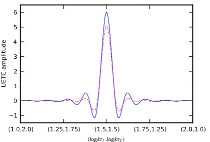
kτ1 ≈ kτ2 (corresponding to the top right corner of Fig. 3 or Fig. 4) there is a ringing pattern with successive positive and negative peaks that decay as we move away from the diagonal. These oscillatory patterns are a consequence of causality [21, 73, 74], built into the USM: as the correlator must vanish at superhorizon scales (in fact in the USM it vanishes at scales larger than the correlation length, which is smaller than the horizon), this introduces a sharp edge in physical space that becomes oscillatory in Fourier space. This oscillatory pattern therefore has a clear physical origin, but in the USM it is somewhat ar-tificially enhanced due to the fact that the model as-sumes all string segments have the same length. If seg-ments are instead given a length distribution peaking at the network correlation length, the sharp edge is smoothed and the oscillatory pattern gets suppressed. Further, considering a segment velocity distribution peaking near the network RMS velocity again sup-presses these oscillations. The Gaussian model as-sumes a wide Gaussian distribution of string lengths (but also assigns non-zero values to the correlator at superhorizon scales) so this causal oscillatory feature is absent from the UETC in that model.

It may also be related to the velocity anti-correlation observed in Nambu-Goto simulations on correlation-length scales and can be attributed to string intercom-mutations [66].

E. Eigenmode Decomposition

The UETC is generally rescaled by a factor of √

τ1τ2, which, forξandvconstant, makes it a function

ofkτ1andkτ2only. This is not true in the present case because now we are tracking the time-dependence ofξ

andv, so the UETC depends separately onk, τ1 and

τ2. However, it is still useful to introduce this rescaling in order to facilitate direct comparison of the UETC with previous results. This rescaled UETC can then be discretised onto a logarithmic grid inkτ1 and kτ2

with n×n grid points and then diagonalised giving the eigenvectors and eigenvalues [19]

(k2τ1τ2)γ

√

τ1τ2hΘ(τ1, k)Θ(τ2, k)i=

N

X

i=1

λiui(kτ1)⊗ui(kτ2). (2.30)

Due to the explicit dependence onk, this diagonalisa-tion procedure has to be repeated for a large number ofk-modes, and the eigenvalues arek-dependent. This significantly increases the computation time compared to [53]. The extra factor (k2τ1τ2)γ is used for more efficient reconstruction of the UETC when the eigen-modes are truncated below n. The choice γ = 0.25 gives the best reconstruction on scales that give the dominant contribution to the CMB anisotropies.

There is no correlation between the scalar, vector and tensor modes and so the vector and tensor UETC can be diagonalised independently. However, the den-sity Θ00, and scalar anisotropic stress ΘS, are

corre-lated. The diagonalisation is done over a 2n×2ngrid constructed from

hΘ00(τ1, k)Θ00(τ2, k)i hΘS00(τ1, k)ΘS00(τ2, k)i

hΘS₀₀(τ1, k)ΘS₀₀(τ2, k)i hΘS(τ1, k)ΘS(τ2, k)i

,

(2.31) where hΘS

00(τ1, k)ΘS00(τ2, k)i is the symmetric

com-bination of the cross-correlation between Θ00 and

ΘS. After diagonalisation, the first half of the eigen-vectors refer to the density and the second to the anisotropic stress. The diagonalisation creates orthog-onal eigenvectors which are then used as source terms in theCAMB[75] linear Einstein-Boltzmann code. The

C` are calculated using each individual eigenvector

ui(kτ)/( √

τ(kτ)γ), as a source functionC_`i, which can be summed to give the total power spectra

C`= n

X

i=1

λiC`i. (2.32) By orderingλifrom largest to smallest, the required accuracy in theC` can be achieved by including rela-tively few eigenmodes. This can be seen in the middle row of Fig.6where there is only about 10% difference between using all 512 eigenmodes of a 512×512 grid

2.0 1.5 1.0 0.5 0.0 0.5 1.0 1.5 2.0

0 4 8 12

2.0 1.5 1.0 0.5 0.0 0.5 1.0 1.5

0.0 0.5 1.0 1.5

2.0 1.5 1.0 0.5 0.0 0.5 1.0 1.5

0.0 0.2 0.4 0.6

2.0 1.5 1.0 0.5 0.0 0.5 1.0 1.5

0.0 0.2 0.4 0.6

2.0 1.5 1.0 0.5 0.0 0.5 1.0 1.5 2.0

2.0 1.5 1.0 0.5 0.0 0.5 1.0 1.5

0.8 0.0 0.8

(1.0,2.0) (1.25,1.75) (1.5,1.5) (1.75,1.25) (2.0,1.0)

( , )

1 0 1 2 3 4 5 6

UETC amplitude

FIG. 5. Profile of the UETC across the diagonal in the oscillatory region with large kτ1 ≈ kτ2. The solid blue line shows the amplitude of the UETC using the value of the velocity and correlation length from the VOS equations whilst the red dot-dot-dash lines has Gaussian distributed velocities and correlation lengths about the VOS values.

compared to only using 32 eigenmodes when fixing the value of Gµ. Also, it can be seen in the top row of Fig. 6 that reducing the grid resolution reduces the amplitude of theC`. A grid resolution of 128×128 is about 5% lower, on average, than using the 512×512 grid but convergence times decrease drastically. It should be noted that there is negligible difference be-tween using a 512×512 and a 1024×1024 grid meaning that the former is reliably giving the full C` contri-bution. The bottom row shows what happens when using more k values in the calculation. Wiggly fea-tures arise from using too few k values and can be removed at the expense of a much longer calculation. Using these findings we can choose the optimal UETC parameters to give good quality C` in a reasonable amount of time. The resulting spectra obtained from our analytical method are shown in Fig. 2 in green dot-dot-dashed curves and agree well with USM string realisations, especially in the limit of large numbers of simulated segments.

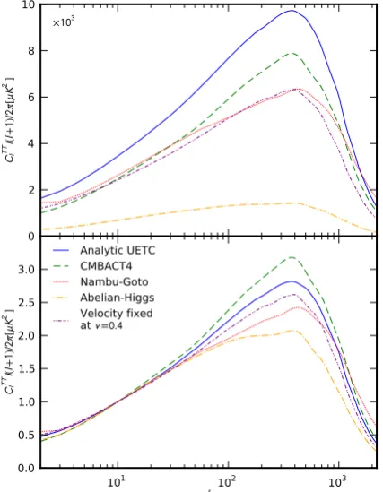
F. Comparison of the String Power Spectrum

In Fig.7 we compare our temperature power spec-trum (scaled by Gµ in the upper subplot and nor-malised at ` = 10) to that of CMBACT4 [61], Nambu-Goto simulations [71], and Abelian-Higgs simula-tions [69]. Both CMBACT4 and our method use the same velocity dependent one-scale model parameters, but CMBACT4 uses Lf = 0.5. The Nambu-Goto sim-ulations are performed in an expanding background from recombination to today, including Λ domina-tion. Large loops are kept in the simulation and con-tribute to the total energy-momentum tensor of the network, but these simulations cannot resolve small-scale physics near the string width and do not include the effects of radiation backreaction. In contrast, the Abelian-Higgs simulations can resolve small-scale structure and radiative effects [76]. These, however, have smaller dynamical range and cannot easily evolve

through the radiation-matter transition (so the UETC is instead interpolated), but see recent progress in [76] where the authors simulate through the transition.

Overall, when normalised at ` = 10, the four spectra agree reasonably well. The USM variants (CMBACT4 and our approach) both predict slightly more power at the peak than either of the simula-tions. The Nambu-Goto simulations predict more power on very small scales, around twice as much as the Abelian-Higgs model. It is well known that Nambu-Goto calculations yield higher string densi-ties than field theoretic ones, which will increase their overall normalisation. The resulting constraints on

Gµare therefore around a factor of 50% lower [33] as can be inferred from the upper subplot in Fig.7. The USM variants are closer to the Nambu-Goto simula-tions in this respect [71]. Within this paper we will not consider using the analytic USM to mimic the Abelian-Higgs spectra. As we have shown, there is some additional uncertainty in the USM, as the nor-malisation depends somewhat on the choice ofLf.

In summary, given the large differences in modelling between the various approaches we find this compar-ison encouraging, although more work is needed to further delineate the differences. In particular, as dis-cussed at the end of Sec. II B, the VOS RMS veloc-ity is defined through a worldsheet integral over all scales and receives a large contribution from relativis-tic wiggles on the string. On the other hand, the USM assumes straight segments moving at a given speed and the small-scale structure on the segments is cap-tured via a “renormalisation” of their tension. This implies that the speed to be associated to the USM segments must be lower than the VOS RMS veloc-ity, and should correspond to the network velocity at correlation length scales. Numerical simulations show this to be significantly lower than the RMS speed. This issue has not been examined before, partly be-cause the calculated string spectra from different ap-proaches can differ by up to a factor of two, and partly because it can be offset by choosing a lower value for the USM parameter Lf (see below). As quantitative agreement between the different approaches is now be-ing established, it is important to fully understand this issue. To this end it will be important to extract the network velocity distribution as a function of length scale in both Nambu-Goto and Abelian-Higgs simula-tions.

101 ₁₀2 ₁₀3

0.0 0.2 0.4 0.6 0.8 1.0

/,

×

101 ₁₀2 ₁₀3

0.0 0.5 1.0 1.5 2.0

/,

×

101 ₁₀2 ₁₀3

0.0 0.5 1.0 1.5 2.0

/,

×

101 ₁₀2 ₁₀3

0.0 0.5 1.0 1.5 2.0

/,

×

101 ₁₀2 ₁₀3

0.0 0.2 0.4 0.6 0.8 1.0

/,

×

101 ₁₀2 ₁₀3

0.0 0.2 0.4 0.6 0.8 1.0

/,

×

101 ₁₀2 ₁₀3

0.0 0.2 0.4 0.6 0.8 1.0

/,

×

101 ₁₀2 ₁₀3

0.0 0.5 1.0 1.5

/,

×

101 ₁₀2 ₁₀3

0.96 0.97 0.98 0.99 1.00 1.01

/,

×

101 ₁₀2 ₁₀3

0.85 0.90 0.95 1.00 1.05 1.10 1.15

/,

×

101 ₁₀2 ₁₀3

0.96 0.97 0.98 0.99 1.00 1.01

/,

×

101 ₁₀2 ₁₀3

0.0 0.5 1.0 1.5

/,

×

FIG. 6. The ratio of theC`calculated using a UETC with a 512×512 grid with all the eigenmodes and: (1. top row)

other grid resolutions, the lightest shaded region with an 8×8 grid whilst the darkest a 256×256 grid; (2. middle row) when fewer eigenmodes are included, 8 eigenmodes for the lightest shaded region and 256 for the darkest; (3. bottom row) when theaccuracy boostsetting ofCAMBis decreased, reducing the number ofk values.

0 2 4 6 8 10

(+

)/

[

]

×

101 ₁₀2 ₁₀3

0.0 0.5 1.0 1.5 2.0 2.5 3.0

(+

)/

[

]

Analytic UETC CMBACT4 Nambu-Goto Abelian-Higgs Velocity fixed at = .

FIG. 7. Comparison of approaches to string modelling, scaled by Gµ in the upper subplot and normalising the temperature power spectrum at ` = 10 in the lower subplot. We compare our approach (in solid blue) to

CMBACT4[61], Nambu-Goto simulations [71], and Abelian-Higgs simulations [69] (in dashed green, dotted red, dot-dashed orange and the analytic USM with the velocity fixed atv= 0.4 in dot-dot-dashed purple respectively).

strings by increasing the string decay rate, thus reduc-ing theC`amplitude and matching simulations better than usingLf = 1. In the absence of a more complete

quantitative understanding of the string velocity dis-tribution - input required from string evolution sim-ulations - our string spectra obtained from the USM have a larger amplitude (see the solid blue line in the upper subplot of Fig.7). This leads to slightly tighter

constraints on cosmic strings than in numerical sim-ulations. Marginalising over the network parameters

cr andα, partly takes care of the differences between

Lf = 0.5 and Lf = 1 in the USM since high cr

re-duces the velocity (as seen from equation (2.16) and pictorially in Fig.1).

III. COSMIC SUPERSTRINGS

A cosmic superstring network can be modelled as a collection of string segments of different types, each string type having its own tension and self-intercommuting probability [44–50, 52, 77–79]. Strings of different types interact with each other via “zipping” or “unzipping” leading to heavier or lighter strings respectively, that are connected to the origi-nal strings at trilinear Y-shaped junctions [80]. The fundamental building blocks for these networks are light (fundamental) F-strings and heavier (Dirichlet) D-strings, with a tension hierarchy controlled by the fundamental string coupling [80–82]. Heavier strings arise as bound states between p F-strings and q D-strings, where p,q are coprime. Given the funda-mental string tension, the corresponding tensions of these heavier (p, q)-strings are controlled mainly by

p,q and the value of the string coupling. These net-works generally behave very differently than their or-dinary cosmic string counterparts. They are typi-cally characterised by small intercommutation prob-abilities, thus leading to higher string number densi-ties [44,45,49,52]. The complex interactions present imply that several string types with different tensions and correlation lengths can simultaneously contribute to the string network CMB spectra.

number of string types considered in the model can be truncated at a finite number. Following [52] we shall describe the network by keeping seven distinct types of strings:

1 F (1,0),

2 D (0,1),

3 F D (1,1),

4 F F D (2,1),

5 F DD (1,2),

6 F F F D (3,1),

7 F DDD (1,3), (3.1)

..

. ... ...

where the last column describes the (p, q) charges of the corresponding string type.

The large-scale dynamics is then modelled by seven copies of the VOS equations, appropriately extended to account for transfer of energy among the different string types through zipping and unzipping interac-tions [44,50]. In each copy of the VOS equations de-scribing a single string, say of typei, the self interac-tion coefficientcrin equation (2.15) is replaced by the corresponding self-interaction coefficient ci, and new cross-interaction terms with coefficientsdk

ij are added to describe zipping and unzipping. The coefficients

ci,dkij are controlled by the corresponding microphys-ical intercommuting probabilities Pij [52], which can be estimated [46, 48] from the corresponding string theoretic amplitudes (and field theory approximations in the case of non-perturbative interactions between heavy strings [47]). They can be expressed as a prod-uct of two pieces: one that is dependent on the vol-ume of the compact extra dimensions Vij(w, gs), and a quantum interaction pieceFij(v, θ, gs). Physically,

one can think of Vij as arising from string position fluctuations around the minimum of a localising po-tential well, giving rise to an effective volume seen by each type of string. The heavier the string the smaller the fluctuations are and so the smaller the value of Vij [46]. The parameter w corresponds to the effec-tive volume in the compact extra dimensions seen by F-strings. gsis the fundamental string coupling andv

andθare the relative velocity and angle of the incom-ing strincom-ings. For a pair of strincom-ings collidincom-ing at an angle

θ, and relative speedv, the intercommuting probabil-ity is

Pij(v, θ, w, gs) =Fij(v, θ, gs)Vij(w, gs). (3.2) Details of how Fij and Vij are calculated can be found in [52]. Since the network contains a large number of individual strings with a range of veloci-ties and orientations, the coefficients ci and dkij are determined by the integral of Pij over a Gaussian velocity distribution centred on the scaling network velocities of each string type and over all angles.

This gives the average intercommuting probabilities Pij(w, gs)≡Pij. Numerical simulations of single-type Nambu-Goto strings with small intercommuting prob-ability [49] suggest that the self-interaction coefficients

ci scale as:

ci=cs×P

1/3

ii , (3.3)

where cs is the standard self-interaction coefficient in three dimensions corresponding to the value cr in Sec.II B. This choice of cs implies a convenient nor-malisation of the coefficients ci so that one recovers the ordinary cosmic string value cr when Pii = 1. This facilitates direct comparison with ordinary cos-mic strings.

For cross-interactions between two strings of types

iandj (i6=j), producing a segment of typek, there is an additional factor arising from the kinematic con-straints of Y-junction formation [83, 84] that we de-note asSk

ij(i6=j). This also arises as an integral over relative velocities and string orientations [52,85]:

S_ijk =1 S

Z 1

0 v2dv

Z π/2

0

sinθdθ

×Θ(−f→

µ(v, θ)) exp[(v−v¯ij)

2_/σ2

v] (3.4) where S is a normalisation factor [52], Θ(−f→

µ(v, θ)) imposes the kinematic constraints [84] and σv2 is the variance of the velocity distribution peaked on the relative scaling velocities ¯vij = (vi2+vj2)1/2 between strings of type i and j. The cross-interaction coeffi-cients are then given by

dk_ij =dij×Skij (3.5) wheredij =κ×P

1/3

ij . The overall normalisationκis the analogue of cs, but for cross-interactions. There

is no obvious choice for this phenomenological param-eter, but it may be expected to be of order unity by analogy to the ordinary self-interacting string result for cr, obtained by numerical simulations. Strictly speaking it should be treated as an extra parameter for the model but, given the large computational re-sources required in our MCMC analysis, we will set it to unity in this work. Our analysis will still indirectly capture the effects of changing this parameter as it is somewhat degenerate with w. To see this, note that dij is also proportional to P

1/3

ij which depends weakly on w through the volume factor Vij(w, gs). The leading effect ofwis to change the relative ampli-tude between self-interactions (FF interactions having the strongestwdependence) and cross-interactions of heavy strings, thus mimicking somewhat the effect of varyingκrelative tocs. As computational power im-proves and our methodology is refined, κ should be re-introduced as an additional MCMC parameter.

ξ_i0= 1 2τ

2v_i2ξiτ

a0

a −2ξi+civi+ X

a,b

db_ia¯viaξi`bia

ξ2

a

−d i ab¯vabξi3`

i ab 2ξ2

aξb2

, (3.6)

v0= v

2₋₁ τ

2viτ

a0

a −

ki

ξi −X

a,b

biab ¯

vab 2vi

(µa+µb−µi)

µi

ξ_i2`i_ab ξ2

aξ2b

, (3.7)

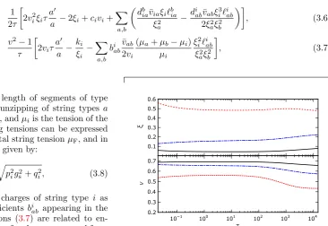
where `i

ab is the average length of segments of type

i formed by the zipping/unzipping of string types a

andbat conformal timeτ, andµiis the tension of the

ith _{string type. All string tensions can be expressed}

in terms of the fundamental string tensionµF, and in

flat spacetime [80–82] are given by:

µi=

µF gs

q p2

ig2s+qi2, (3.8) where pi and qi are the charges of string type i as listed in (3.1). The coefficients bi_ab appearing in the velocity evolution equations (3.7) are related to en-ergy conservation and allow for the enen-ergy saved from zipping interactions to be redistributed as kinetic en-ergy of the new segment (bi

ab=d i

ab) [50] or radiated away (bi_ab = 0) as in [44]. A more realistic model should have a specific radiation mechanism so that 0 < bi

ab < diab such that some of the energy is redis-tributed whilst the rest is radiated away. However, for cosmic superstring networks (for which dij are much smaller than unity) this term has negligible impact on the string scaling densities and velocities [52, 85], so here we takebi

ab= 0.

Once the velocities and correlation lengths of all string types in the network are obtained by solv-ing (3.6-3.7), their unequal-time correlators can be calculated independently as laid out in Sec. II. Al-though N > 3 string types are needed in order to accurately construct the abundances of the domi-nant three lighter strings (in this case seven string types are used (3.1)), the resulting scaling densities of the higher charged states withN >3 are strongly suppressed compared to the lighter F-, D- and FD-strings [44, 50, 85]. This allows us to only consider these first three states in the computation of CMB signatures through our UETC analytic method. The evolution of the network parameters for the three lightest strings can be seen in Fig. 8 for cs = 0.23,

w= 1 and gs= 0.3.

Once the UETC of each of the three lighter strings are calculated they can simply be summed to give the total string UETC, since the individual segments are uncorrelated in the USM. This can then be diag-onalised and the eigenvectors and eigenmodes used as sources for finding the contribution from cosmic super-strings to the CMB anisotropy. We have checked that our analytic UETC method reproduces the results of Fig. 4 in [52], including the shift in the location of the peak as we vary gs. We have found a slightly lower amplitude in the B-mode spectrum that can be at-tributed to the extra factor of 2 in the vector modes

0.1 0.2 0.3 0.4 0.5 0.6

10 1 ₁₀0 ₁₀1 ₁₀2 ₁₀3 ₁₀4

v

0.2 0.3 0.4 0.5 0.6 0.7

ξ

τ

FIG. 8. The radiation and matter era evolution of the velocity v, and correlation length ξ, for the F-string in solid black, D-string in dot-dashed blue and FD-string in dotted red. These results are obtained when gs = 0.3, w= 1 andcs= 0.23.

that was present inCMBACT3(which [52] was based on) and has been corrected inCMBACT4[86].

IV. STRING CONSTRAINTS

We obtain joint constraints on cosmic string net-work and ΛCDM parameters using a modified version ofCOSMOMC. To reduce computational time in our anal-ysis we have tested two methods for deriving string network constraints. In the first method, the string

C` are pre-calculated for a range of cr = [0.1,1] and α = [1,10] at the Planck best fit values for the cos-mological parameters, i.e. Ωbh2, Ωch2andH0. These C`are read intoCOSMOMC, interpolated at the MCMC

cr and α values and then scaled by (Gµ)2_{. This is}

an extremely efficient way for obtaining network con-straints since only the ΛCDM C` need to be calcu-lated, while the interpolation takes very little time. We have checked that the difference in the resulting string C` when calculated at the upper and lower 3σ bounds in Ωbh2, Ωch2 and H0 is ∼0.5% in the

tem-perature, E- and B-modes and no more than∼10% in the TE cross-correlation. This uncertainty in the stringC`is1% of the totalC`. TheC`for different

cr andαare plotted in Fig. 9. The different bands of colour indicate the value ofcr, solid red being the low-est (cr = 0.1) then progressing through long-dashed

flattening the small`features (as best seen in the sec-ond column and to a lesser extent in the third column of Fig.9). Increasingcrreduces the amplitude of the

C` and, as best seen in the third column of Fig. 9, shifts the main peak towards slightly smaller `. In the second method, which is computationally expen-sive, we simply calculate the string and ΛCDMC`for each (network) parameter value and compare to CMB data.

The same process of pre-calculating string spectra can be done for cosmic superstring networks in the parameter ranges cs = [0.1,1], gs = [0.01,0.9] and

w = [0.001,1]. The superstring C` can be seen in Fig.10, where same colours and patterns are used for the steps incs as in Fig. 9. The bands indicate

val-ues ofw, withw = 10−3 corresponding to the solid-patterned lines andw= 1 to the dotted version of the same pattern. The rows indicate varying values ofgs, with gs = 0.01, gs = 0.1 and gs = 0.9 for the top, middle and bottom rows respectively. The first point to notice is that theC`amplitudes at lowgsare much greater than those at largegs. For largecsvalues there is less difference between the greatest and smallest values of w, especially at lowgs, i.e. the purple dot-dash-dotted lines in the top row of Fig.10overlap, but are well separated in the bottom row. This is because for largecs the cross-interaction termsdk_ij (which are less dependent on w than the self-interaction terms

ci) play a more important role in setting the scaling string number densities. For small values ofcs, theci coefficients become smaller (while dk

ij are unaffected) leading to small correlation lengths and so large string number densities. The C` amplitudes are then af-fected more strongly by ci, giving rise to a stronger dependence onw.

The datasets used in the MCMC analysis come from the Planck2015 mission [41], in particular: Planck2015 TT+lowP: This contains the 100-GHz, 143-GHz, and 217-GHz binned half-mission TT cross-spectra for`= 30−2508 with CMB-cleaned 353-GHz map, CO emission maps, and Planck catalogues for the masks and 545-GHz maps for the dust residual contamination template. It also uses the joint tem-perature, E and B cross-spectra for ` = 2−29 with E and B maps from the 70-GHz LFI full mission data and foreground contamination determined by 30-GHz LFI and 353-GHz HFI maps.

Planck2015 TT+Pol+lowP: This contains the same data as Planck2015 TT+lowP but also uses the TE and EE cross-spectra for`= 30−1996.

Planck2015 TT+Pol+lowP+BKPlanck: This again contains all of the data used in Planck2015 TT+Pol+lowP but includes also the cross-frequency spectra between BICEP2/Keck maps at 150 GHz and Planck maps at 353 GHz including the B-mode spec-tra at multipoles`∼50−250.

We first consider our interpolation method, where the C` are pre-calculated on a grid in cr and α (or in the case of cosmic superstring networkscs, gs and

w), and then a spline interpolation used between grid

values. The results obtained from this method are very quick and accurate due to our ability to use all 512 eigenmodes of the 512×512 grid for the UETC. The constraints on network parameters derived from this method are shown in Fig.11. Gµis implemented into the MCMC analysis through a logarithmic prior of [−10,−5] such thatGµ= 10[−10,−5].

There is no significant difference in our constraints when using Planck2015 TT+lowP, or including EE and TE or both EE and TE and BB results. The up-per 2σ value for the tension is Gµ < 1.1×10−7 for Planck2015 TT and is similarlyGµ <9.6×10−8 _and Gµ <8.9×10−8 _{for Planck2015 TT+Pol+lowP and}

Planck2015 TT+Pol+lowP+BKPlanck. These agree well with theGµ <1.8×10−7 _{and Gµ <1.3×10}−7

from the Planck cosmological parameters analysis [33]. The slightly tighter constraints obtained here are due to the amplitude of theC`not scaling with the value of

Lf, i.e. theC`are larger whenLf= 1 as assumed here, while previous results were obtained fromCMBACTwith

Lf = 0.5. There is little difference between using the Planck temperature data alone and including polari-sation data as expected from [33]. As can be seen in the other two columns of Fig.11,crandαare not con-strained. There is a slight preference for higher values of cr and lower values of α since both of these lead

to smaller C`. Features, such as the position of the main peak or the pronounced lower`peak make very little difference to the overall constraints. There is a very slight correlation between Gµ and cr and

anti-correlation between Gµand α, as expected from the

C` seen in Fig. 9. A combination of high αand low

cr is mildly disfavoured. Further, by comparing the constraints on Gµandcr to their affect on theC` in Fig.9 there is a larger difference between changes at smallcr than changes at largecr. For this reason we

expect to see greater correlation between Gµ and cr

on a logarithmic scale from valuescr1 tocr≈0.1 than implied over our prior range.

Considering our direct calculation method, where the string spectra are calculated every time along with theC` from ΛCDM, the constraints are slightly weaker. This is because there is a pay-off between the resolution of the UETC and number of eigenmodes used in the reconstruction and the time spent com-puting the spectra. To efficiently calculate the con-straints a grid resolution of 128×128 with 64 eigen-modes has been used. As can be seen in Fig. 6 we expect a reduction in power of about 10−20% which means the value of Gµ is allowed to be higher than when the high resolution, full reconstruction interpo-lation method is used. For Planck2015 TT+lowP this isGµ <4.3×10−7. The constraints oncrandαalso show a slight preference for lowercr and largerα, as in our interpolation method.

For cosmic superstrings, GµF, gs and w are

101 ₁₀2 ₁₀3 100 101 102 103 104 105 (+ )/ [ ]

101 ₁₀2 ₁₀3

10 5

10 4

10 3

10 2

101010

101 102 103 (+ )/ [ ]

101 ₁₀2 ₁₀3

10 5

10 4

10 3

10 2

10101 0 101 (+ )/ [ ]

101 ₁₀2 ₁₀3

2.0 1.5 1.0 0.5 0.0 0.5 (+ )/ [ ] ×

FIG. 9. The totalC` (scalar+vector+tensor modes) for different values ofcr andα. The red solid lines showcr = 0.1

and through yellow (long-dashed), green (short-dashed), blue (dot-dashed) and purple (dot-dash-dotted) forcr = 0.3, cr = 0.5,cr= 0.7 andcr = 0.9. The upper (solid-patterned) lines indicateα= 10 whilst the lower (dotted versions of the pattern) lines are forα= 1. This is shown forC`T T,C

EE ` ,C

BB ` andC

T E

` in columns 1-4.

101 ₁₀2 ₁₀3

104 105 106 107 (+ )/ [ ]

101 ₁₀2 ₁₀3

100 101 102 103 104 105 (+ )/ [ ]

101 ₁₀2 ₁₀3

100 101 102 103 104 (+ )/ [ ]

101 ₁₀2 ₁₀3

2.5 2.0 1.5 1.0 0.5 0.0 0.5 (+ )/ [ ] ×

101 ₁₀2 ₁₀3

102 103 104 105 (+ )/ [ ]

101 ₁₀2 ₁₀3

10 1 100 101 102 103 (+ )/ [ ]

101 ₁₀2 ₁₀3

10 2 10 1 100 101 102 (+ )/ [ ]

101 ₁₀2 ₁₀3

2.5 2.0 1.5 1.0 0.5 0.0 (+ )/ [ ] ×

101 ₁₀2 ₁₀3

10 1 100 101 102 103 (+ )/ [ ]

101 ₁₀2 ₁₀3

10 4

10 3

10 2

10101 0 101 (+ )/ [ ]

101 ₁₀2 ₁₀3

10 5 10 4 10 3 10 2 10 1 100 (+ )/ [ ]

101 ₁₀2 ₁₀3

2.5 2.0 1.5 1.0 0.5 0.00.5 (+ )/ [ ] ×

FIG. 10. The totalC` obtained from cosmic superstrings for different values ofgs,cs andw. As with previous figures,

the first column shows the temperature auto-correlationC`, the second the EE, third the BB and the last column shows

the temperature, E-mode correlationC`. The three rows showgsvalues of 10−2, 10−1 and 0.9 from top to bottom. The

colouring and patterning system is the same as in Fig.9with red (solid), yellow (long-dashed), green (short-dashed), blue (dot-dashed) and purple (dot-dash-dotted) lines indicating the values ofcs fromcs= 0.1 to 0.9 in steps of 0.2. The width of the band of similar colour and pattern indicates the upper and lowerwvalues with the dotted-patterned lines defined byw= 10−3 and the solid-patterned lines byw= 1.

be found in Fig. 12. It can be seen that w and cs

are almost flat (columns 3 and 4), again with larger values of cs favoured as this leads to smaller am-plitude C`. As the string density grows with de-creasing gs, the constraints on gs favour larger

val-ues, as seen in the second column. Note, however, that the model is not reliable for large values of gs

as the perturbative expansion starts to break down and the string interaction amplitudes used in ci and

dk

ij have large uncertainties. Finally, the first column shows our constraints on the fundamental string ten-sionGµF, which is much smaller than for ordinary cos-mic strings. We findGµF<2.8×10−8_{for Planck2015}

TT+lowP when marginalising over gs, cs andw, and the same constraint for Planck2015 TT+Pol+lowP and Planck2015 TT+Pol+lowP+BKPlanck.

Also in Fig. 12 we show the constraints when us-ing the direct calculation method, where the strus-ing spectra are calculated at every step in the Markov chain. This is a much more intensive computation

and so a lower resolution grid and fewer eigenmodes in the reconstruction had to be used. As for cosmic strings the optimal balance between computing time and accuracy suggested using a 128×128 grid with 64 eigenmodes. The constraints are thus slightly weaker, with the main resultGµF<4.2×10−8. The results from our two methods are in good agreement, justify-ing the use of our interpolation method, and showjustify-ing that varying ΛCDM parameters within Planck priors has little effect on the string constraints.

V. CONCLUSIONS

stochas-8 6 4 2 0.6 0.8 0.4

0.2 10-6

10-7

10-8

10-9

10-10

2 4 6 8 0.2 0.4 0.6 0.8

cr α

Gµ

α

cr

Planck2015 TT+lowP Planck2015 TT+Pol+lowP Planck2015 TT+Pol+lowP +BKPlanck

Planck2015 TT+lowP - Direct

FIG. 11. 2σlikelihood contours forGµ,crandαfrom the stringC`interpolation and direct calculation methods. The

or-ange line shows the constraints from Planck2015 TT+lowP, purple and blue lines are used for Planck2015 TT+Pol+lowP and Planck2015 TT+Pol+lowP+BKPlanck respectively. The black dashed line shows the direct calculation constraints for Planck2015 TT+lowP.

tic background which can be constrained using pul-sar timing, laser interferometry experiments such as LIGO and eLISA, and also the CMB [87]. A tran-sient gravitational wave signal is also expected from cusps and kinks in the network [88]. The latter class of tests has the potential to provide even stronger con-straints on the string tensionGµ, but there are large uncertainties in the loop size, which is fixed by itational back-reaction. Model dependence on grav-itational waves from cosmic strings further makes it difficult to determine signatures, for example, whilst Nambu-Goto strings decay into loops, Abelian-Higgs strings primarily decay into particles [88–90]. It is therefore important to use a variety of complemen-tary observational probes.

The first class of tests also suffer from uncertain-ties, but these are less significant. The string UETC can be obtained from simulations and used as source functions in CMB codes, but simulations are numer-ically expensive and suffer from issues in dynamical range. An alternative approach is to model the string network as an ensemble of segments using the USM. Crucially, although the USM provides a simplified pic-ture of the network, it is able to match simulations by adjusting the free parameters of the model, namely the correlation length, RMS velocity and string

wig-gliness.

In this paper we have significantly improved and extended our previous work on string power spectra from the USM:

1. We have analytically solved the UETC for an evolving string network, whereas our previous work was restricted to constant network param-eters. The UETC itself can be computed in under a minute. For the CMB power spec-trum, although the time taken is increased due to tracking a larger number of Fourier modes, on a 3.1 GHz Intel Xeon CPU with 8 threads, our code runs in∼60 minutes. For comparison, around 2000 network realisations are required for CMBACT4 to achieve the same accuracy and since this code is serial, the computation time is ∼30 hours.

0.4 0.2 0.0

10-1

10-2

10-3

10-1

10-2

10-7

10-8

10-9

10-10

0.2 0.4 0.6 0.8

10-3

10-2

10-1

10-1

0.6 0.8 1.0

cs

10-2

w

gs

w

GµF

cs gs

Planck2015 TT+lowP

Planck2015 TT+Pol+lowP

Planck2015 TT+Pol+lowP +BKPlanck

Planck2015 TT+lowP - Direct

FIG. 12. 2σlikelihood obtained forGµF,gs,wandcs. The black dashed line (and black shading) shows the constraints from Planck2015 TT+lowP direct calculation method and orange, purple and blue lines are the Planck2015 TT+lowP, Planck2015 TT+Pol+lowP and Planck2015 TT+Pol+lowP+BKPlanck constraints using the interpolation method.

3. For the first time we have been able to marginalise over the string network parameters when fitting to Planck2015 and joint Planck-BICEP2 data. The data is consistent with no strings for both the single and multi-string case. Since other network parameters are un-constrained when the tension is very small, it is only possible to present joint constraints on these with Gµ. In the superstring case, for ex-ample, the constraint on the string coupling gs

is degenerate withGµF.

There are several possibilities to explore in future work. Firstly, there are various ways in which the USM could be improved. Superstring networks con-tain Y-type junctions, but in the present formulation these only impact the evolution of the network pa-rameters. Since junctions are relatively rare in the limit of large and small coupling, the USM is expected to provide a sufficient description. However, in some

regimes the energy density of the network may not be dominated by a single string type, and junctions may become important. In this case the USM could be modified to include a correlation between segments. A further improvement is the inclusion of loops. The decay of string segments in the USM should mimic the energy loss in loops, but it is possible these may lead to additional interesting signatures.

line-of-sight. This has already been demonstrated for the CMB bi-spectrum [92] by performing many realisa-tions of the network. It is possible to employ a simi-lar analytic method used in this work to compute the string bi- and tri-spectrum, which we would expect to be significantly faster [93].

The detection of gravitational waves by LIGO is particularly exciting for strings, and the next genera-tion of ground and space based experiments can po-tentially provide much stronger limits than those from the CMB. However, these limits strongly depend on modelling, for example, the loop, kink and cusp dis-tribution. Further work is needed to understand these and until then the CMB will continue to be an impor-tant tool in the search for strings.

ACKNOWLEDGEMENTS

We appreciate useful conversations with Richard Battye, Levon Pogosian, Carlos Martins and Jon Ur-restilla. We also thank Martin Kunz, Andrei Lazanu and Paul Shellard for the use of their string spectra. TC is supported by an STFC studentship. The work of AA is supported by an Advanced Research Fellow-ship at the University of Nottingham. AM is sup-ported by a Royal Society University Research Fellow-ship. EJC is supported by STFC Consolidated Grant ST/L000393/1. We are grateful for access to the Uni-versity of Nottingham High Performance Computing Facility. Finally, we thank the referee for their invalu-able comments on this paper.

[1] T. W. B. Kibble, Phys. Rept.67, 183 (1980). [2] A. Vilenkin and E. Shellard, Cosmic Strings and

Other Topological Defects, Cambridge Monographs on Mathematical Physics (Cambridge University Press, Cambridge, 2000).

[3] M. Hindmarsh, Nucl.Phys. B392, 461 (1993), arXiv:hep-ph/9206229.

[4] E. J. Copeland and T. W. B. Kibble, Proc. Roy. Soc. Lond.A466, 623 (2010),arXiv:0911.1345.

[5] E. J. Copeland, L. Pogosian, and T. Vachas-pati, Class. Quant. Grav. 28, 204009 (2011), arXiv:1105.0207.

[6] D. Baumann, A. Dymarsky, I. R. Klebanov, and L. McAllister, JCAP 0801, 024 (2008), arXiv:0706.0360.

[7] C. Burgess, M. Majumdar, D. Nolte, F. Quevedo, et al., JHEP0107, 047 (2001),arXiv:hep-th/0105204. [8] E. J. Copeland, A. R. Liddle, D. H. Lyth, E. D. Stew-art, et al., Phys.Rev.D49, 6410 (1994), arXiv:astro-ph/9401011.

[9] G. Dvali, Q. Shafi, and R. K. Schaefer, Phys.Rev.Lett.

73, 1886 (1994),arXiv:hep-ph/9406319.

[10] G. Dvali and S. H. Tye, Phys.Lett.B450, 72 (1999), arXiv:hep-ph/9812483.

[11] S. Kachru, R. Kallosh, A. D. Linde, J. M. Mal-dacena, et al., JCAP 0310, 013 (2003), arXiv:hep-th/0308055.

[12] A. D. Linde, Phys.Rev.D49, 748 (1994), arXiv:astro-ph/9307002.

[13] E. J. Copeland, R. C. Myers, and J. Polchinski, JHEP

0406, 013 (2004),arXiv:hep-th/0312067.

[14] R. Jeannerot, J. Rocher, and M. Sakellari-adou, Phys.Rev. D68, 103514 (2003), arXiv:hep-ph/0308134.

[15] S. Sarangi and S. H. Tye, Phys.Lett. B536, 185 (2002),arXiv:hep-th/0204074.

[16] R. H. Brandenberger, Phys.ScriptaT36, 114 (1991). [17] C. Contaldi, M. Hindmarsh, and J. Magueijo, Phys.Rev.Lett. 82, 679 (1999), arXiv:astro-ph/9808201.

[18] T. Kibble and N. Turok (1985).

[19] U.-L. Pen, U. Seljak, and N. Turok, Phys.Rev.Lett.

79, 1611 (1997),arXiv:astro-ph/9704165.

[20] A. Albrecht, R. A. Battye, and J. Robin-son, Phys.Rev.Lett. 79, 4736 (1997), arXiv:astro-ph/9707129.

[21] A. Albrecht, R. A. Battye, and J. Robin-son, Phys.Rev. D59, 023508 (1998),

arXiv:astro-ph/9711121.

[22] P. Avelino, E. Shellard, J. Wu, and B. Allen, Phys.Rev.Lett. 81, 2008 (1998), arXiv:astro-ph/9712008.

[23] R. A. Battye, J. Robinson, and A. Albrecht, Phys.Rev.Lett. 80, 4847 (1998), arXiv:astro-ph/9711336.

[24] E. J. Copeland, J. Magueijo, and D. A. Steer, Phys.Rev. D61, 063505 (2000), arXiv:astro-ph/9903174.

[25] I. Gott, J. Richard, Astrophys.J.288, 422 (1985). [26] N. Kaiser and A. Stebbins, Nature310, 391 (1984). [27] L. Pogosian, S. H. Tye, I. Wasserman, and

M. Wyman, Phys.Rev. D68, 023506 (2003),

arXiv:hep-th/0304188.

[28] M. Wyman, L. Pogosian, and I. Wasserman, Phys.Rev. D72, 023513 (2005), arXiv:astro-ph/0503364.

[29] R. Battye and A. Moss, Phys. Rev. D82, 023521 (2010),arXiv:1005.0479.

[30] C. Dvorkin, M. Wyman, and W. Hu, Phys.Rev.D84, 123519 (2011),arXiv:1109.4947.

[31] B. Shlaer, A. Vilenkin, and A. Loeb, JCAP1205, 026 (2012),arXiv:1202.1346.

[32] P. Ade et al. (Planck), Astron.Astrophys. 571, A25 (2014),arXiv:1303.5085.

[33] P. A. R. Ade et al. (Planck) (2015),arXiv:1502.01589. [34] J. Lizarraga, J. Urrestilla, D. Daverio, M. Hind-marsh, et al., Phys. Rev. D90, 103504 (2014), arXiv:1408.4126.

[35] N. Bevis, M. Hindmarsh, M. Kunz, and J. Urrestilla, Phys.Rev.D76, 043005 (2007),arXiv:0704.3800. [36] P. Mukherjee, J. Urrestilla, M. Kunz, A. R.

Liddle, et al., Phys.Rev. D83, 043003 (2011), arXiv:1010.5662.

[37] L. Pogosian and M. Wyman, Phys.Rev.D77, 083509 (2008),arXiv:0711.0747.

[38] U. Seljak, U.-L. Pen, and N. Turok, Phys.Rev.Lett.

79, 1615 (1997),arXiv:astro-ph/9704231.

[39] U. Seljak and A. Slosar, Phys.Rev. D74, 063523 (2006),arXiv:astro-ph/0604143.

[40] J. Urrestilla, P. Mukherjee, A. R. Liddle, N. Be-vis, et al., Phys.Rev. D77, 123005 (2008), arXiv:0803.2059.

[41] N. Aghanim et al. (Planck), Submitted to: Astron. Astrophys. (2015),arXiv:1507.02704.