Development and testing of an experimental power system fault demonstrator

Development and testing of an experimental power system fault

demonstrator

C. Rose

_{, D. W. P. Thomas, M. Sumner, E. Christopher}

∗_{University of Nottingham, UK, [email protected]}

Keywords: Protection; power distribution systems; fault demonstration; fault location; experimental demonstrator.

Abstract

In this paper a laboratory demonstrator for the study of power system faults is described. The facility has been developed in order to experimentally investigate a number of fault loca-tion and power system protecloca-tion technologies developed by the authors and their colleagues at higher power levels and with more representative system parameters than has previ-ously been possible. In addition to describing the facility itself, this paper also describes the validation of a previously studied method using the new demonstrator.

1

Introduction

Reliable fault location is desirable in electrical transmission and distribution systems as well as more electric ships and air-craft: automated fault location allows the correct circuits to be isolated while minimising the impact on other parts of the sys-tem, and accurate knowledge of where a fault has occurred can substantially reduce repair times [1–3]. In addition, the study of novel equipment and control methods under fault conditions is an important stage of development, as it demonstrates the be-haviour of the design under abnormal conditions and can show compliance with relevant grid standards [4–6]. Although it is possible to perform studies on operating power systems – and such studies are of considerable value – results from this type of field testing are not always easily reproduced under con-trolled conditions and the occurrence of faults and transients is generally unpredictable. As a consequence, fault testing at the early stages of development is often done through simulation or using supplies with limited power availability, as is the case in [7–9].

This paper describes a new power system fault demonstrator, designed specifically to validate a number of fault location al-gorithms, but also suitable for studying the behaviour of grid-connected equipment under faulted conditions, in a controlled environment where repeatable results may be achieved. Also in this paper, results are presented to validate a fault location method [9] at higher voltage and current levels than has previ-ously been possible. The accuracy of the method is considered and some of the potential sources of error are identified.

2

The experimental demonstrator

The power system fault demonstrator is built around a laboratory-based microgrid at the University of Notting-ham [10]. The demonstrator may be powered from a num-ber of AC or DC sources in either a grid-connected or isolated mode, and the design is such that the supply impedance may be varied and faults of varying types and severity may be ap-plied at a number of locations. The experimental power sys-tem consists of a variable impedance supply connected to a main feeder which links five cabinets, each consisting of the switchgear and protection required to control the loads con-nected to that cabinet. Each section of the main feeder consists

of 10 m of 16 mm2 _{cable. A photograph of the experimental}

facility is shown in Figure 1. The system is illustrated as a one-line diagram in Figure 2.

Fig. 1: Photograph of the experimental facility.

Fig. 2: One line diagram showing the demonstrator layout.

of three-phase inductors with numerous tap positions,

allow-ing the inductance to be varied up to2mH and variable

high-power resistor banks providing up to2 Ωof additional supply

resistance.

Current and voltage transducers are installed in the first and last cabinets, referred to as Zone 1 and Zone 5 respectively. The installed current transducers are hall effect type sensors

with a±300A input range [11], although the data acquisition

hardware will saturate when the measured current magnitude

exceeds250 A. The transducers may be upgraded to allow

higher fault currents to be accurately measured. The voltage

transducers are differential voltage probes with a±700V input

range [12], however, the output of the probes is limited to 70% of the input range of the sampling hardware. The transducer outputs are sampled using 16-bit analogue to digital

convert-ers, giving theoretical resolutions of0.0038A for the current

transducers and0.0153V for the voltage transducers, which is

a considerably higher resolution than required. At present the maximum allowable fault current is determined by the range of the current transducers.

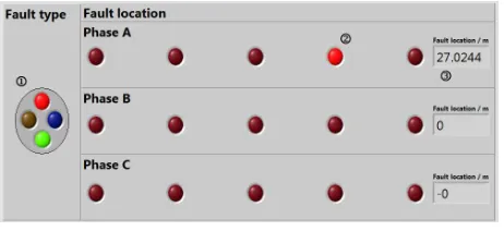
Fig. 3: A screenshot of the user interface showing: (1) the fault

type indicator, (2) the fault location indicators, (3) the fault location readout.

Data capture and processing is handled using a National Instru-ments Compact RIO (cRIO) [13], which contains an FPGA

and microprocessor for data capture, processing and control. The cRIO was programmed using LabView. Data acquisition is performed continuously at a sampling frequency of 50 kHz. Captured data is then filtered and downsampled to 12.5 kHz us-ing the FPGA. A user interface is provided through a PC. The user interface displays the cRIO output in a human-readable format. Figure 3 shows the important parts of the user in-terface. The three key features of the interface are the fault type indicator, the fault location indicator and the fault location readout. The fault type indicator shows the type of fault de-tected by illuminating the indicators associated with the faulted cores of the cable: red, yellow and blue for Line 1, Line 2 and Line 3 respectively and green for the neutral/earth conductor. The fault location indicator gives an immediate, visual indica-tion of which secindica-tion of cable is faulty, and the locaindica-tion readout gives the estimated distance from the beginning of the line to the fault in metres. The “back-end” of the cRIO software may be configured to implement a number of different fault location methods. In addition to displaying the fault location results, the cRIO also saves the recorded transient data to a file, which may be retrieved using the cRIO’s network interface and im-ported for viewing and analysis using suitable software, such as MATLAB.

In order to impose faults on the system a number of fault units were constructed. The units consist of a contactor connected to the power system on one side and to a miniature circuit breaker (MCB) and a number of shorting links on the other. The fault units can be configured by inserting or removing the shorting links. The MCB ensured eventually disconnection of the fault, even in the event of contactor failure. A fault unit is connected to each of the five cabinets. The faults may be triggered from a control panel consisting of a number of switches, each con-trolling one of the fault units. Figure 4 shows one of the fault units.

Fig. 4: Photograph of one of the fault units.

the units are first activated is similar to what may be expected from an arc fault; this is caused by the arcing which occurs in-ternally as a result of “switch-bounce” as the contactor closes. This can be seen in Figure 5, which shows a typical fault tran-sient captured by the cRIO, where it takes approximately 2 mS for the voltage to settle after the fault occurs. The effect is also visible to a lesser extent in the current waveform.

0 0.002 0.004 0.006 0.008 0.01 0.012 0.014 0.016 −200

−100 0 100 200 300 400

Voltage (V)

0 0.002 0.004 0.006 0.008 0.01 0.012 0.014 0.016 −200

−100 0 100 200

Time (s)

Current (A)

Fig. 5: Typical captured fault transient data.

This section has described the design of the experimental fault demonstrator. Testing of the demonstrator and validation of a fault location algorithm have been carried out and this is de-scribed in the next section.

3

Fault location methodology

The fault location method used during testing of the facility is a double-ended technique, described in detail in [14]. The method uses current and voltages measurements taken at the sending and receiving ends of the line. Continuous data cap-ture is performed for all transducers as described in the previ-ous section.

Fig. 6: Equivalent circuit used to derive the fault location

al-gorithm.

When a fault is detected, 5.1 mS of additional data is captured. This is combined to the last 5.1 mS of captured data prior to the fault to give a total of 10.2 mS of data to be analysed. For this work, a basic threshold trigger was used to detect the fault. Captured voltages and currents are preprocessed using a Black-man window to remove the discontinuities at the start and end of the data. An equivalent circuit of a faulted power system is shown in Figure 6. Using Kirchoff’s Laws to analyse the equivalent circuit it can be seen that the impedance from the

supply to the fault,Zsf, may be calculated using (1).

Zsf =

Vr−Vs+IrZsr

Is+Ir

(1)

Once the impedance has been estimated at a number of fre-quencies an ordinary least squares curve fit is applied between 0 Hz and 3000 Hz. The quality of captured data above 3000 Hz was found to deteriorate rapidly and was therefore ignored. The resistive part of the results is ignored as it is assumed that the fault will be primarily resistive. The curve-fitted reactance results are then used to calculate the cable inductance between the supply and fault. The distance from the supply to the fault may then be calculated by dividing the estimated inductance by the per unit-length cable inductance.

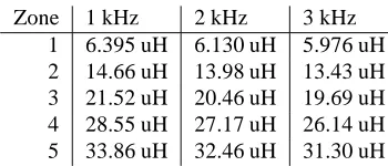
Zone 1 kHz 2 kHz 3 kHz

1 6.395 uH 6.130 uH 5.976 uH

2 14.66 uH 13.98 uH 13.43 uH

3 21.52 uH 20.46 uH 19.69 uH

4 28.55 uH 27.17 uH 26.14 uH

5 33.86 uH 32.46 uH 31.30 uH

Table 1: Calibrated fault reactance results.

0 0.002 0.004 0.006 0.008 0.01 −100

0 100 200 300

Time (s)

Voltage (V)

0 0.002 0.004 0.006 0.008 0.01

−300 −200 −100 0 100

Time (s)

Current (A)

0 500 1000 1500 2000 2500 3000

0 0.1 0.2

Frequency (Hz)

Resistance (

Ω

)

0 500 1000 1500 2000 2500 3000

0 0.2 0.4 0.6

Frequency (Hz)

Reactance (

Ω

)

Fig. 7: Full results showing the captured transient supply voltage and current and the estimated impedance for a single-phase to

earth fault. The dotted lines on the impedance results are the results after curve fitting.

available. The line inductance was therefore measured using a four-wire impedance analyser for calibration purposes [15]. In addition, the fault inductances were also measured using the impedance analyser. Calibration measurements were taken at 1000 Hz, 2000 Hz and 3000 Hz for a fault in each of the five zones. Results of the calibration tests are shown in Table 1. The reactance of the whole line is equal to the line reactance seen when a fault occurs in Zone 5 and is therefore not sep-arately listed. Some variation in inductance with frequency is seen. It is not yet clear if this is a measurement error or an actual variation (the cable capacitance is negligible at these frequencies and therefore not the cause). The quality of the fault location results appear to be unaffected by this variation. From the calibration results the cable inductance was found to

be approximately0.82µHm−1_{. The DC cable resistance was}

measured and is equal to3.8mΩm−1_.

3.1 Experimental results

Testing of the algorithm was performed a number of times for faults in each location. Individual results were considered in order to identify sources of error and to determine if any im-provements to the signal processing could be made. The over-all quality of the fault location results was also considered, by analysing the variation in results between tests. The results are presented below.

Figure 7 shows a typical set of results for a single-phase to neu-tral fault in Zone 5. The fault occurs at approximately 5 mS, resulting in a sharp drop in voltage accompanied by a rapid

rise in current. The average resistance is0.143 Ω, which is

reasonably close to the expected value of0.152 Ωfor a fault

in this zone. Using the curve-fitted results for calculation, the

inducatance is found to be30.2µH, slightly lower than the

ex-pected value of32.8µH, but still within 10%. The fault is then

calculated to be37.3m from the supply.

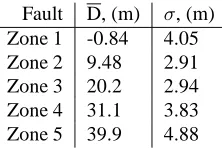
In order to evaluate the overall performance of the algorithm, 40 tests were completed for a phase to neutral fault at each fault location. The mean estimated distance-to-fault, D, and

the standard deviation,σ, of the results were calculated using

the results for each fault location and used to judge the efficacy of the algorithm. The statistical summary of the results is given in Table 2.

Fault D, (m) σ, (m)

Zone 1 -0.84 4.05

Zone 2 9.48 2.91

Zone 3 20.2 2.94

Zone 4 31.1 3.83

Zone 5 39.9 4.88

Table 2: Mean estimated distance-to-fault and standard

devia-tions for each zone.

The calculated averages are close to their expected values. From these results it would appear that absolute error in the estimated distance to fault is smallest when the fault occurs near the middle of the line and greatest at the ends of the line. Relative errors are greatest at the supply end of the line and reduce as the fault approaches the load end of the line. The relative errors for results within one standard deviation of the mean in Zones 3, 4 and 5 is already only slightly above 10%. For Zone 2 the error is closer to 20%. The relative error for a fault in Zone 1 is high; this is not unexpected however, since the expected estimated distance for a fault in Zone 1 is very small. Absolute error for Zone 1 is comparable to the absolute errors for Zones 4 and 5.

addressing these errors an overall accuracy of better than 10% may be consistently achieved using the fault location method described.

3.2 Sources of error

0 0.002 0.004 0.006 0.008 0.01 0.012 −300

−250 −200 −150 −100 −50 0 50

Tims (s)

Voltage (V)

0 0.002 0.004 0.006 0.008 0.01 0.012 −50

0 50 100 150 200 250

Tims (s)

Current (A)

Fig. 8: An example of poorly triggered results. The results

should be centred around the fault transient. The tran-sient occurs very close to the voltage zero-crossing, at about 3 mS, but is not detected until 5.1 mS.

Some of the errors are due to limitations in the fault detection method. The simple threshold trigger which is applied to the measured currents successfully detects all faults; however, if the fault occurs close to the voltage zero crossing, the current will not exceed the threshold until part-way through the next half cycle. As a result, the triggering of the fault location al-gorithm is delayed and the captured data is not centred around the fault transient. In addition to the delayed triggering, the fault transient is also less significant than for faults occurring near the peak voltage, reducing the amplitude of the transient frequency content used for fault location. This can be seen in Figure 8.

An improved trigger method for the fault location algorithm may improve results but is also likely to be more susceptible to normal system transients. Work is ongoing to find and evaluate a suitable alternative trigger method.

For some results it was found that the fault transients did not contain sufficient frequency content at certain frequencies for accurate reactance estimates to be obtained. This was gener-ally a problem at higher frequencies. The physical cause of this phenomenon is not yet understood. It should be possible

to overcome this problem by narrowing the range of frequen-cies used for the curve fitting. However, an optimum upper frequency limit has not yet been found.

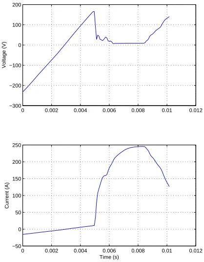
During testing it was found that the choice of MCB used in the fault units has a significant impact on the quality of results. In some cases, it was found that the MCBs in the fault units would trip within a half-cycle of the fault occurring, corrupting the captured data and resulting in unreliable results. The cap-tured fault transient when the MCB tripping current is too low is shown in Figure 9. The early opening of the MCB causes the voltage to recover and the fault current to fall. Early dis-connection of the faults is another significant source of error in the results, although obviously not a practical concern with regards to the protection of real systems.

Using MCBs with higher trip currents is the most obvious so-lution to this problem, although this should be done with care. The MCB trip current must be low enough to ensure discon-nection within a few cycles if the fault does not disconnect, but should not be so low as to disconnect the fault immediately. The ratings of the fault unit MCBs have been increased and it is hoped that testing with the revised fault unit design shall be completed soon.

0 0.002 0.004 0.006 0.008 0.01 0.012 −300

−200 −100 0 100 200

Voltage (V)

0 0.002 0.004 0.006 0.008 0.01 0.012 −50

0 50 100 150 200 250

Current (A)

Time (s)

Fig. 9: A captured fault transient, showing the MCB opening

4

Conclusions

This paper has described the design of an experimental fault demonstration facility and the implementation and evaluation of a fault location algorithm. Test results have been presented to demonstrate the method used, which uses relatively low fre-quency transient voltages and currents to estimate the fault lo-cation. Some of the sources of error created by the test pro-cedure have been discussed. Work is ongoing to eliminate or reduce errors where possible. Additional testing is planned to demonstrate the fault location algorithms for DC systems. Testing of the demonstrator with a DC supply is expected to take place in the near future.

Future work is also planned focussing on arc faults. For paral-lel arc fault studies only relatively minor modifications to the demonstrator are deemed to be necessary as the test methods are similar to those already presented in this report. The au-thors are also aware of a method of locating series arc faults al-though some significant modifications to the demonstrator will be necessary before it is possible to study this method further.

5

Acknowledgements

The authors would like to thank Nottingham Technology Ven-tures for funding the construction of the fault demonstrator.

References

[1] M. M. Saha, J. J. Izykowski and E. Rosolowski, “Fault

Location on Power Networks,” Springer-Verlag London, 2010

[2] Yanfeng Gong, M. Mynam, A. Guzman, G. Benmouyal

and B. Shulim, “Automated fault location system for non-homogeneous transmission networks,” Protective Relay Engineers, 2012 65th Annual Conference for, pp.374-381, 2-5 April 2012

[3] Chen Yu, Liu Dong, Xu Bingyin and Huang Yuhui,

“Wide area travelling wave fault location in the transmis-sion network,” Electricity Distribution (CICED), 2010 China International Conference on, pp.1-6, 13-16 Sept. 2010

[4] S. Loddick, U. Mupambireyi, S. Blair, C. Booth, X. Li,

A. Roscoe, K. Daffey, and J. Watson, “The use of real time digital simulation and hardware in the loop to de-risk novel control algorithms,” Electric Ship Technolo-gies Symposium (ESTS), 2011 IEEE, pp.213-218, 10-13 April 2011

[5] J. Niiranen, ”Experiences on voltage dip ride through

factory testing of synchronous and doubly fed generator drives,” Power Electronics and Applications, 2005 Euro-pean Conference on,

[6] N. Bottrell and T. C. Green, ”Comparison of

Current-Limiting Strategies During Fault Ride-Through of Invert-ers to Prevent Latch-Up and Wind-Up,” Power Electron-ics, IEEE Transactions on, vol.29, no.7, pp.3786-3797, July 2014

[7] J. Wang, P. Kadanak, M. Sumner, D. W. P. Thomas and

R. D. Geertsma, “Active fault protection for an AC zonal marine power system architecture,” The 2008 IEEE in-dustry applications society annual meeting (IAS 2008), 5-9 October 2008

[8] Ke Jia, David Thomas and Mark Sumner, “Single-ended

fault location scheme for utilization in integrated power system,” Power Delivery, IEEE Transactions on, vol.28, no.1, pp.38-46, Jan. 2013

[9] Ke Jia, David Thomas and Mark Sumner, “A New

Double-Ended Fault-Location Scheme for Utilization in Integrated Power Systems,” Power Delivery, IEEE Trans-actions on, vol.28, no.2, pp.594-603, April 2013

[10] R. Davies, A. Fazeli, Sung Pil Oe, M. Sumner, M.

John-son and E. Christopher, “Energy management research using emulators of renewable generation and loads,” In-novative Smart Grid Technologies (ISGT), 2013 IEEE PES, pp.1-6, 24-27 Feb. 2013

[11] Multicomp, “Current Transducer”, datasheet,

http://www.farnell.com/datasheets/1368151.pdf

[12] Pico Technology Ltd., “TA041 25MHz +/-700V

Differential Probe User’s Manual”, datasheet,

http://www.farnell.com/datasheets/83434.pdf

[13] National Instruments Corporation, “What is NI

CompactRIO”, webpage, last accessed 23/04/2015, http://www.ni.com/compactrio/whatis/

[14] Ke Jia, “Impedance based fault location in power

distri-bution systems”, PhD thesis, University of Nottingham, 2011

[15] Newtons4th Ltd. “LCR Active Head and Impedance

Analysis Interface”,