Munich Personal RePEc Archive
Financial Bubble Detection : A
Non-Linear Method with Application to
SP 500
Michaelides, Panayotis G. and Tsionas, Efthymios and
Konstantakis, Konstantinos
2016
Online at
https://mpra.ub.uni-muenchen.de/74477/
1
FINANCIAL BUBBLE DETECTION: A NON-LINEAR
METHOD WITH APPLICATION TO S&P 500
Panayotis G. Michaelides1
National Technical University of Athens
Efthymios G. Tsionas
Lancaster University
Konstantinos N. Konstantakis
National Technical University of Athens
Abstract
The modeling process of bubbles, using advanced mathematical and econometric techniques, is a young field of research. In this context, significant model misspecification could result from ignoring potential linearities. More precisely, the present paper attempts to detect and date non-linear bubble episodes. To do so, we use Neural Networks tocapture the neglected non-linearities. Also, we provide a recursive dating procedure for bubble episodes. When using data on stock price-dividend ratio S&P500 (1871.1-2014.6), employing Bayesian techniques, the proposed approach identifies more episodes than otherbubble tests in the literature, while the common episodes are, in general, found to have a longer duration, which is evidence of an early warning mechanism (EWM) thatcouldhave important policy implications.
Keywords:Bubbles, Non-linearities, Neural Networks, EWM, S&P500
JEL Classification: C5, G1
1 Laboratory of Theoretical and Applied Economics; School of Applied Mathematical and Physical Sciences; National
2
FINANCIAL BUBBLE DETECTION: A NON-LINEAR
METHOD WITH APPLICATION TO S&P 500
1.
Introduction
In August 2015,the Chinese stock market lost over 30% of its stock value,
experiencing one of the worst stock market crashes in recent financial history.
Despite the efforts made by the Chinese Government and the Chinese Central
Bank to prevent the crash by implementing a strict legislatory framework on
short selling as well as by providing huge cash injections to brokers so as to
stimulate stock demand, the Shanghai Stock Exchange experienced an
unprecedented crash. As a result, on the 24th of August, the Shanghai Stock
Exchange experienced an overall devaluation of approximately 8% in stock
prices, the so-called “Black Monday” of the Chinese Stock Market (The New
York Times, 25 August 2015).
Despite the fact that in the long history of financial bubbles the Chinese
case isnot the first and certainly not the last one, only limited attention has
been paid by the scientific community tocreatingarigorous androbust
framework for the detection of bubble formationbased on a credible Early
Warning Mechanism (EWM).In general, EWMs are essential components of
time-varying macroprudential policies that can help reduce the high losses
associated with both banking and country specific crises. In this context, the
EWMs employed should not only have sound statistical forecasting power,
but also need to satisfy several additional requirements.
Analytically, the importance of bubble dating lies on the appropriate
timing, which is a crucial requirement for EWMs. In this context,
macroprudential policies need time before they become effective (Basel
Committee 2010) and, hence, signals should need to arrive at a relatively early
stage in order to prevent policy measures from being costly (Caruana 2010).
3 precisely, policy makers tend to base decisions on trends rather than reacting
to changes in signaling variables immediately (Bernanke 2004). Meanwhile,
the gradual implementation of policy measures may also allow policy makers
to affect market expectations more efficiently and deal with uncertainties in
the transmission mechanism (CGFS 2012). Finally, a last requirement is that
EWM signals should be easy to interpret, as any signals that do not “make
sense” are likely to be ignored by policy makers (Önkal et al 2002; Lawrence
et al 2006). In sum, well designed EWIs, in terms of timing and signal
processing, can reduce uncertainty and allow for more decisive policy action.
Thus far, one of the main reasons behind the inability of most models
to capture the formation of bubbles,at a relatively early stage, is the fact that
bubble formation has inherent non-linear characteristics,which are difficult to
capture using standard linear models. This, clearly, implies that any
econometric test that aims at capturing the formation of bubbles, especiallyat
an early stage, should be able to capture their non-linear character.
Additionally, another equally important challenge for the econometric
detection of bubbles is their dating, in the sense that an econometric test
should be able to accurately date the bubble periods detected in the sample.Of
course, early detection and accurate dating of financial bubbles could have
important policy implications, especially for central bankers and policy
makers since it could assist in the implementationofrelevant policy actionsthat
could potentially ease the consequences of bubbles. More specifically, the
importance of early identification lies in the timing of specific
countermeasures that could potentially prevent: a) the magnitude of a
potential collapse through regulatory interventions in the financial markets;
b) the potential downturn effects of bubble collapse in the economy through
appropriate inflation targeting, and c) the devastating spillover effects in the
global economy through interest rate and/or exchange rate setting.
Due to the fact that, according to the recent financial history of bubbles,
4 any econometric test for bubble detection should be structured upon flexible
backward and/or forward recursive estimation techniques.However,
relatively limited research has been done in the literature using recursive
estimation techniques for dating multiple bubble episodes. See Phillips and
Yu (2011), and Phillips et al. (2011a, 2011b, 2013, 2014, 2015a) and Phillips et
al. (2015b) [hereafter PSY].
Meanwhile, nonlinear economic models have become quite popular
lately, because economic data exhibit significant non-linearities. To this end,
in this paper, we propose a rigorous and robust mathematical and
econometric framework for the detection of bubbles, which is structured upon
ArtificialNeuralNetworks (ANN),that are perfectly capable of capturing any
neglected non-linearity. In fact, this is the first paper in the relevant literature,
to the best of our knowledge, which employs ANNs, to capture neglected
non-linearities in bubbles.
After all, according to PSY, the use of computationally efficient dating
methods “over long historical periods presents a more serious econometric
challenge due to the complexity of the nonlinear structure and break mechanisms that are inherent in multiple-bubble phenomena within the same
sample period”. Finally, our approach provides a recursive algorithm for the
accurate detection of bubbles, which serves as an EWM that could be used in
order to guide a policy decision in an uncertain environment, without the
need of taking into consideration the policy maker’s preferences (e.g.
Pesaranand Skouras 2002; Granger and Machina 2006; Baxa et al. 2013). In brief, the present paper contributes to the literature in the following
ways: (a) It establishes a rigorous framework, based on ANNs, under which
bubble detection could be achieved, while emphasizingonthe presence of
non-linearities; (b) It provides a new algorithm for the accurate and early detection
of bubble formation, as well as for the identification of potential explosive
behaviors; (c) it illustrates the proposed testby early detecting and capturing
5 time period 1871 (M1)-2014 (M6), and by identifying more episodes compared
to a competitive methodology in the literature.
This paper is structured as follows:insection 2, a review of the literature
takes place; section3 presents the theoretical model; section 4 sets out the
proposed non-linear test; section 5presents the empiricalanalysis;finally,
section 6concludes.
2.
Related Literature
According to Kindleberger (1978) a bubble is defined as “an upward price
movement over an extended range that then implodes”. Brunnermeier (2009)
argued that bubbles “are typically associated with dramatic asset price
increases followed by a collapse”, whereas Garber (2000) defined a bubble as
the part of the price movement that cannot be explained by fundamentals.
Also, Barlevy (2007) described a bubble as “a situation where an asset´s price
exceeds the fundamental value of the asset”. In brief, a bubble occurs when
the market value is higher than the fundamental (Diba and Grossman 1988).
Some researchers (e.g. Wu 1997) define bubbles as the difference between the
fundamental value and the market price allowing, thus, for negative bubbles.
Reasons for the occurrence of bubbles include, among other things, greed
(Kindleberger 1978), introduction of breakthrough technologies or financial
innovations (e.g. Perez 2009);existence ofrational and irrational traders
(Dufwenberg, Lindqvist and Moore 2005; Hong, Scheinkman andXiong2007);
institutional restrictions on short selling (Haruvy and Noussair, 2006);
herding(DeMarzo, Kaniel and Kremer 2008), speculating investors
(Greenwood and Nagel 2005; Scheinkman and Xiong2002), and “bubble
riding” (Abreu and Brunnermeier 2003, and Temin and Voth 2003).
Despite the fact that several approaches, even seminal ones (e.g. Fama,
1965), have denied the possibility of bubbles in financial markets, the
[1634-6 1637], Mississippi Bubble [1719–1720]) and has often led to generalized and
deep economic recessions. As a result, Fama’sEfficient Market Hypothesis and other similar theories have not always found so much support. After all,
probably the most prominent economist, who considered the existence of
bubbles in financial markets, was John Maynard Keynes (1936).
Following the related literature on financial bubble detection,Shiller (1981)
and Lerroy and Porter (1981) were probably the first to develop variance
bound tests for equity prices. Despite the fact that Shiller’s (1981) variance
bound test was not initially developed for bubble detection, the works of
Blanchard and Watson (1982) and Tirole (1985) suggested that violation of
variance bounds could be attributed to the presence of bubbles. Nevertheless,
the variance bound tests were heavily criticized by a number of authors
likeFlavin (1983), Mash and Merton (1983), Mankiw et al. (1985), Kleidon
(1986) and Flood et al. (1994), due to the fact that the variance bound tests
could fail not only if bubbles exist but also if any of the assumptions of the
present value model is violated.
In a different approach, West (1987) developed a two-step test for the
identification of bubbles in equity prices based on Euler’s equation of no
arbitrage process and the autoregressive process of dividends that governs
the market fundamental stock price. Despite the fact that West’s (1987) test
was more attractive than the variance bound test as it explicitly incorporated
the null hypothesis of no bubbles, once again Dezbakhsh and Demirguc-Kunt
(1990), as well as Flood et al. (1994), criticized the econometric procedure of
the test because it exhibited significant size distortions in small samples.
Another popular approach for bubble detection was the one proposed
by Diba and Grossman (1987, 1988a, 1988b),who tried to exploit the
theoretical properties of bubbles. Their test allowed for unobserved
fundamentals in the market fundamental price and a bubble would exist if the
7 However, Evans (1991) criticized the test of Diba and Grossman (1988b)
byarguingthat it was unable to capture a periodically collapsing bubble.
Following Evans (1991), a vast literature emerged concerning the
detection of bubbles, like Hall and Sola (1993), van Norden (1996), van
Norden and Vigfusson (1998), Driffil and Sola (1998), and Hall et al. (1999)
who incorporated regime switching models for bubble detection. In the
meantime,in a seemingly unrealtedapproach, Wu (1997) used Kalman
filtering in an attempt to test for bubbles, while Wu and Xiao (2002) tried to
establish a test for bubbles based on the residuals of the cointegrating
equation between dividends and stock prices.
This signified the formation of the latest strand in the literature of bubble
detection where researchers based the existence and detection of bubbles on
the unit root behavior of key fundamental financial variables. In a prominent
paper, Phillips and Yu (2011) introduced a recursive regression methodology
in order to analyze the bubble characteristics of various financial time series
during the subprime crisis. Phillips et al. (2011a) extended the work of
Phillips and Yu (2011) by introducing a relevant econometric framework
where more than one bubbles could exist in the same sample. Phillips et al.
(2011b) provided the identification conditions regarding the explosive
behavior of bubbles based on the unit root behavior of relevant financial time
series.
Breitung and Holmes (2012) investigated the power properties of
rational bubbles considering a large variety of testing alternatives, while
Breitung and Kruse (2013) showed that structural break Chow-type tests have
considerable power for the detection of bubbles. Again, Phillips et al. (2013)
illustrated their proposed bubble specification and dating algorithm using
data from S&P500 series, while Phillips et al. (2014) provided the asymptotic
8 in two seminalworks,Phillips et al. (2015a) and PSYprovided probably the
only framework, thus far, in the existing literature, under which an EWM is
established for the detection of multiple bubble episodes.
3.
The Theoretical Model
From a technical point of view, probably the most important feature of
bubbles is that they are characterized by explosive growth patterns, despite
the fact that speculative movements are often assumed to follow a random
walk process (e.g. Blanchard and Watson 1982, Campbell, Lo, and MacKinlay
1997). And it is exactly this, the most common way to identify a bubble, by
applying tests for a structural change from a random walk regime to an
explosive one. Such tests have been developed by Phillips, et al. (2011a),
Phillips and Yu (2011), Homm and Breitung (2012), Phillips et al. (2014), and
PSY.
3.1
Time Series Model
From a technical perspective, the identification of bubbles involves the use of
key financial time series variables, such as dividends, stock prices, equity
prices etc.
For any financial time series variable, ݔ௧ೕǡ ݆ א ܬ, we will make a number of
fairly standard assumptions:
Assumption 1: The time series xtis assumed to conform to the standard
additive component model, i.e. every financial time series variable ݔ௧ǡ ݅ א ܫ,
9
ݔ௧ ൌ ݏ௧ ݃௧ ܿ௧ ߝ௧, ݅ א ܫ(1)
where: ݏ௧ is the seasonal component, ݃௧ is the trend component, ܿ௧ is the
cyclical component and ߝ௧̱ܰሺͲǡ ߪଶሻ is the error term.
For the sake of simplicity, and without loss of generality, we also make the
following assumption:
Assumption 2: The trend and constant term of the series ݔ௧ǡ ݅ א ܫ, are both
assumed to be equal to 0.
In case, (deterministic) terms are to be considered, the standard procedure is
to apply demeaning and detrending procedures before computing the
relevant test statistics.
Now, we present the general formulation of the unit-root test upon
which the econometric testing of bubbleswill be based.
Assumption 3: The unit root detection is described by the following model:
߂ݔ௧ൌ ߩݔ௧ିଵή ܩሺݔ௧ିଵǢ ߛሻߝ௧ǡ ݐ ൌ ͳǡ Ǥ Ǥ Ǥ ǡ ܶǡ ݅ א ܫ(2)
whereߝ௧̱ܰܫܦሺͲǡ ߪଶ) and G is a sufficientlysmooth function.
With reference to the aforementioned general specification, without
deterministic components, the most popular unit root test in the literature, i.e.
the traditional Dickey Fuller (D.F.) test, is based on the ݐ-statistic of ߩfrom the model:
10 The null hypothesis, ܪ, of a unit root is parameterized by ߩ ൌ Ͳ.
The vast majority of empirical tests in the literatureare based on
alternative forms of the D.F. test above (Equation 3). However, some other
unit root testing attempts are also present in the literature, where researchers
have attempted to capture bubbles based onsomenon-linearunit root
specification.More precisely, Kapetanios et al. (2003) or KSS extended thestandardapproach on unit root testing through the introduction of a
so-called exponentialsmooth transition autoregressive (ESTAR) model and
decided to consider the following ESTAR process, emphasizing the expected
low power of the linear augmented D.F. test, when applied to such a series:
߂ݔ௧ൌ ߛݔ௧ିଵ൛ͳ െ ൫െߠݔଶ௧ିଵ൯ൟ ߝ௧), ݅ א ܫ(4)
The analysis of KSS focuses on ߠ, with ܪͲǣߠ ൌ Ͳand ܪͳǣߠ Ͳ. AsDŽis
unidentified under ܪͲǡ ߠ ൌ Ͳcannot be tested. Hence, they based their work
onLuukkonenetal. (1988) and employed a first-order Taylor series
approximation to the ESTAR model under the null ܪͲǣߠ ൌ Ͳ. The relevant
equation is:
߂ݔ௧ൌ ߩݔଷ௧ିଵߝ௧, ݅ א ܫ(5)
where the nonlinear test relies on the t-statistic of ǒfrom the O.L.S. regression on the previous equation.
However, it should be noted that the aforementioned models (i.e.
linear, or ESTAR, etc)are not grounded on some formal mathematical or
statistical criterion, but rather on the modeling choices of each individual
researcher. Therefore, both attempts that are equivalent to the assumption
11 For instance, changing the degree of the implied polynomial assumed
in the aforementioned ESTAR process would lead to another exponential
power of the relevant test.Hence, misspecification issues arise from ignoring
potential nonlinear terms. As a result, it would seem absolutely imperative to
test for the presence of nonlinear terms.
In this work, in order to overcome these serious drawbacks which
result from the arbitrarily assumptions about the processes to be followed,
instead of fitting the Gfunction with a pre-specified equation, we will use an Artificial Neural Network (ANN) to let the dataset itself serve as evidence to
support the model’s approximation of the underlying specification.
3.2ANNs Formulation
As we have seen, the main idea is to express the arbitrary specification
߂ݔ௧ൌ ߩݔ௧ିଵή ܩ൫ݔ௧െ ͳǢ ߛ൯ǡ ݅ א ܫnot as a pre-specified form based on a priori
assumptions, but rather let the dataset itself determine the specification of
the underlying process. In other words, instead of fitting ߂ݔ௧ with a
pre-specified functional form, ANNs let the dataset itself serve as evidence to
support the model’s approximation of thespecification.In what follows, we
proceed by providing a formal definition of ANNs.
Definition1: ANNs are collections of functions that relate an output variable
Y to certain input variables ࢄᇱൌ ሾܺଵǡ ǥ ǡ ܺெሿ. The input variables are
combined linearly to form N intermediate variables ܼଵǡ Ǥ Ǥ Ǥ ǡ ܼே ࢆே ൌ
ܺԢߚሺ݇ ൌ ͳǡ ǥ Ǥ ǡ ܰሻ, where ߚ א Թேare parameter vectors. The intermediate variables are combined non-linearly to produce Y:
ܻ ൌ σேୀଵܽ߮ሺ߄ሻ(6)
12 We make use of a single layer ANN to avoid computational and
energetic requirements (see Sanger 1989).Hence, it is worth mentioning that
the mechanism behind ANNs is that they combine simple units with
intermediate nodes, so they can approximate any smooth nonlinearity (Chan
and Genovese 2001). In fact, ANNs provide very good approximations to a
large class of arbitrary functions while keeping the number of parameters to
a minimum(Hornik et al. 1989, 1990). Also, they can approximate their derivatives, a fact which justifies their success (Hornik et al. 1990, Brasili and Siltzia 2003).
To sum up, ANNs are data-driven and self-adaptive, nonlinear
methods that do not require specific assumptions about the underlying
specification (Zhang and Berardi 2001). In addition, theyare universal
approximators of functions.In this paper, we useaANN formulation in order
tocaptureand model nonlinearities in bubbles.
3.3 Mathematical Properties
As we have seen in the previous section, the main idea for capturing a
financial bubble episode is to thoroughly investigate the respective unit root
behavior of the financial time series variable. To this end, using the general
specification of unit root detection, i.e.߂ݔ௧ ൌ ߩݔ௧െ ͳή ܩ൫ݔ௧െ ͳǢ ߛ൯ǡ ݆ א ܬwe will
formally approximate the function G, using anANN. To do so, we will make
use of the formal definitions of open set, open covering, compact set, dense set
and closure (e.g. Rudin, 1976)that will help us formally stateour main
Theorems,below. In what follows, we will make use of Hornik’s
(1991)Theorem (see Theorem 1, Appendix), whichstates the conditions under
which anANN specification can approximate any given function.
In simple words, according to Hornik’s (1991) Theorem,ANN’s that are
based on non-constant, continuous and bounded activation functions are
capable of approximating any smooth function as long as the domain of the
13 (Definition 2, Appendix), which constitutes the domain of the function, and
then we prove that this set could be considered as being compact (see
Theorem 2).
Theorem 2: If ݔ௧ǡ ݅ א ܫǡ is an arbitrary time series, such that ݔ௧א Թ݅ א ܫand
ݐ א ܶ andthe set of time seriesڂ ݔאூ ௧ ؿԹ, is closed and bounded, thenڂ ݔאூ ௧ is a compact subset of ԹǤ
Proof: See Appendix.
Please note that the implicit assumptions made for the time series set is
that it is closed and bounded. The financial time series set could be
considered as being closed since it could contain all its boundary points.
Additionally, we consider the financial time series set to be bounded since all
financial time series couldhave a finite time dimension.
Next, in order to be able to apply Hornik’s(1991) Theorem, we also
need to formally prove that the proposed specification, for the unknown
function G of the general unit root specification, possesses all the mathematical properties that Theorem 1 explicitly states. Below, Theorem 3
formally presents the proposed functional specification and proves the
relevant properties.
Theorem 3: Ifݔ௧ǡ ݅ א ܫ is an arbitrary time seriesand the set of time series
ڂ ݔאூ ௧ ؿԹis a compact subset of Թ, whereas ߮ǣԹ՜ Թ is a non-constant,
bounded and continuous function, then any function݇ǣ Թ՜ Թ of the form
݇ሺݔ௧ିଵሻ ؠ ߩݔ௧ିଵڄ ܨሺݔ௧ିଵሻ, ߩ א Թ,ݐ א ܶ, where: ܨ൫ݔ௧ିଵ൯ ؠ σேୀଵܽ߮ሺߚڄ ݔ௧ିଵሻ,
withܽ,ߚא Թ݊ א Գ, and ܽ0, for some݊ א Գ, is also continuous, bounded
14
Proof: See Appendix.
Having formally shown that the proposed specification is fully
compatible with Hornik’s(1991) Theorem, below we state our main result
(Theorem 4), which states that the specification can formally approximate
arbitrarily well the generalnon-linear specification.
Theorem 4
If the set ڂ ݔאூ ௧ ؿԹ, ݐ א ܶ is a compact subset of Թ, then the family of
functions ࣠ ൌ ሼ݇ሺݔ௧ିଵሻ א ൫ڂ ܩא ൯ǣ ݇ሺݔ௧ିଵሻ ؠ ߩݔ௧ିଵڄ ܨሺݔ௧ିଵሻ , ܨ൫ݔ௧ିଵ൯ ؠ
σேୀଵܽ߮ሺߚڄ ݔ௧ିଵሻ, withܽ, ߚא Թ݊ א Գ,ߩ א Թሽisdense in the set of
functions ൌ ڂ ܩא
Proof: See Appendix.
In simple words, Theorem 4 implies that the proposed specification
݇ሺݔ௧ିଵሻ ؠ ߩݔ௧ିଵڄ ܨሺݔ௧ିଵሻ , ܨ൫ݔ௧ିଵ൯ ؠ σேୀଵܽ߮ሺߚڄ ݔ௧ିଵሻ , with ܽ , ߚא Թ݊ א Գ,ߩ א Թisa global approximator to any arbitrary specification ǒxt-1ڄG(x t-1; DŽ) and, hence, the proposed specification could approximate arbitrarily well the general non-linear unit root specification.
4.
The Test
As PSY have emphatically pointed out,the econometric identification of
non-15
linear structure involved in the multiple breaks that produce the bubble phenomena. This is the reason why a general nonlinear ANN approximation is used in this work as the main mechanism in the proposed econometric test.
4.1
Formulation
We have formally, shown thatthe proposed specification݇ሺݔ௧ିଵሻ ؠ ߩݔ௧ିଵڄ
ܨሺݔ௧ିଵሻ,ܨ൫ݔ௧ିଵ൯ ؠ σேୀଵܽ߮ሺߚڄ ݔ௧ିଵሻ, withܽ, ߚא Թ݊ א Գǡ ߩ א Թis a
global approximation to any arbitrarynon-linearunit root specification,
i.e.ߩݔݐ െ ͳ ڄܩሺݔݐ െ ͳǢ ߛሻ. Therefore, ݅ א ܫǡthe general unit root test of the form
߂ݔ௧ൌ ߩݔ௧ିଵ ڄܩ൫ݔ௧ିଵǢ ߛ൯ ߝ௧ could be approximated arbitrarily well by the
test ߂ݔ௧ ൌ ݇൫ݔ௧ିଵ൯ ߝ௧, where ߝ௧satisfies the usual assumptions.2 In detail, exploiting the proposed NN specification, the relevant testing equation
becomes:
߂ݔ௧= σேୀଵߩܽݔ௧ିଵڄ ߮ሺݔ௧ିଵǢ ߚሻ,݅ א ܫ(7)
Now, without loss of generality,wecansafely make an additional simplifying
assumption about the behavior of the employed time series.
Assumption 4: ݔ௧ represents time series of the form:ݔ௧ൌ ሺ
షభሻ.
For instance, ݔ௧would naturally represent the logarithmic return of asset
prices between two time periods in time t and t-1, e.g. daily. As a result,
ݔ௧ ൌ ൬
షభ൰ ǡ ݔ௧א ܤሺͲǡ ߝሻǤ
2
It should be noted that lag augmentation, in case of serial dependence, does not affect either the test or its mathematical derivation. On the contrary, lags of the dependent variable may indeed be included to eliminate serial correlation.
16 This is due to the fact that the quantity (before taking natural
logarithms) ǣ
షభא ܤሺͳǡ ߝሻǡ
షభ א ܤሺͳǡ ߝሻ , even for
large daily fluctuations in pricesܲ௧. However, it should be noted that large
daily fluctuations in pricesܲ௧ are extremely improbable, even in developing
markets.Additionally, we have to make an assumption about the activation
function ߮ of the ANN.
Assumption 5: Without loss of generality,we may assume, that the activation
function of the ANN has the following form:
߮ሺݖ௧ሻ ൌ ݁௭ഁെ ͳ(8)
It should be noted that߮ሺݖ௧ሻis continuous,non-constant and bounded when
ݖ௧ א ܤሺͲǡ ߝሻ, andǃ is a positive real number.
Of course, it should also be pointed out that other alternative activation
functions could be used. See Bishop (1995). However, in general, the empirical
results are robust, regardless of the activation function used (Haykin, 1999).
In this work, and given the complexity of the problem, the chosen
function is able to transform the model to one which lends itself to empirical
estimation, contrarily to other possible activation functions. In this sense, the
argument by Kuan and White (1994) is in force: ‘‘given the popularity of
linear models in econometrics, this form is particularly appealing, as it
suggests that ANN models can be viewed as extensions of, rather as
alternatives to, the familiar models”.
Now, based on equation (8), equation (7) takes the following form:
߂ݔ௧ൌ σ ߩܽݔ௧ିଵڄ ሾ݁௫షభ ഁ
ே
17 In what follows, we will make use of Taylor’s expansion Theorem, to
get an equivalent but more convenient form, of the term:
݁௫షభഁെ ͳ(10)
Thus, by applying the aforementioned Theorem around ݔൌ Ͳ, we get that:
݁௭ഁൎ 1+ݖ௧ఉ(11)
Hence, takinginto consideration equation (11), equation (9) becomes:
߂ݔ௧=ߩܽଵݔ௧ିଵڄ ൣͳ ݔ௧ିଵఉభെ ͳ൧ ߩܽଶݔ௧ିଵൣͳ ݔ௧ିଵఉమെ ͳ൧ ڮ ߩܽݔ௧ିଵൣͳ ݔ௧ିଵఉೖെ ͳ൧ ڮ ߩܽேݔ௧ିଵڄ ൣͳ ݔ௧ିଵఉಿെ ͳ൧
߂ݔ௧ = ߩܽଵݔ௧ିଵఉభାଵ+ߩܽଶݔ௧ିଵఉమାଵ+…+ߩܽேݔ௧ିଵఉಿାଵ, ݅ א ܫ(12)
Now, without loss of generality,݊ א Գ,let: ߩܽൌ ߢ and ߚ ͳ=ߜ. Thus, we
get:
߂ݔ௧ = ߢଵڄ ݔ௧ିଵఋభ + ߢଶڄ ݔ௧ିଵఋమ + …+ߢேڄ ݔ௧ିଵఋಿ,݅ א ܫ(13)
With the inclusion of the error term, we have the following test:
Proposition 1:The null hypothesis, ܪ, of a unit root is parameterized bya test
ofσேୀଵߢൌ Ͳ, ߜא ȁܤሺͳǡ ߝሻȁ, ߝ Ͳ, n = 1,2,…Nin:
߂ݔ௧ = ߢଵڄ ݔ௧ିଵఋభ + ߢଶڄ ݔ௧ିଵఋమ + …+ߢேڄ ݔ௧ିଵఋಿ +ߝ௧,݅ א ܫ(14)
Proof: See Appendix.
It is worth noting that equation (14)could beseen as a generalization of KSS.
Now, following PSY and the relevant strand in the literature, the
previous model specification is complemented with transient dynamics, just
as in standard ADF unit root testing. Hence,the proposed specification takes
the form:
18 Of course, in order to allow application of the test with intercept, or intercept
and trend terms included, these deterministic terms are removed via preliminary regression with the demeaned or detrended version of ݔ௧.
4.2
Existence of Bubbles
In what follows,we propose a generalized max NNUnit Root (NNUR) test for the presence ofbubbles, as well as a recursive forward and backward
technique,based on Bayesian Methods, to detect and time-stamp the bubble
origination and termination dates, where flexible window widths are used in
their implementation.
Instead of fixing the starting point of the recursion on the first
observation, the proposed test extends the sample coverage by changing both
the starting point and the ending point of the recursion over a feasible range of
flexible windows and is, therefore, suited to analyzing long historical data
(PSY).
Now, following the literature on the econometric detection of
bubblesas set out earlier, we may make the following assumption:
Assumption 6: ݅ א ܫ the error term, ߝ௧̱ܰሺͲǡ ߪ௧ଶሻ, where ߪ௧ଶfollows a GARCH
process of the form:ߪ௧ଶ ൌ ݃൫ߪ௧ଶିଵǡ ߝ௧ିଵଶ൯ ൌ ܽ ܽଵߪ௧ଶିଵ ܽଶߝ௧ିଵଶ(16)
where: ܽ Ͳǡ ܽଵ Ͳǡ ܽଶ Ͳ.
In what follows, we performrepeated NNUR tests on sub-samples of
the data on a recursive, backward and forward manner, changing the starting
and ending points. We proceed by providing a simple algorithmfor the
implementation of the test, regarding the detection of bubbles in a time frame.
The following simple algorithm sets out the mechanism behind the proposed
19
Step 1:Let݅ א ܫ, and ݔ௧ an arbitrary time series of length ܶ Ͳ and consider a
sample of it, the so-called window ܹ with length Ͳ ൏ ܹ ൏ ܶ.
Step 2:Partitionthe sample ܹ into all the possible sub-samples ݎ௪ೕ ൌ
ሾݎଵೕǡ ݎଶೕሿ ك ܹ where ݎଵೕ is the starting date of the j-th sub-sample and ݎଶೕ the
respective ending date. In this way, we obtain the set of all subsamples
ݎ௪ൌ ڂ ݎא ௪ in W.
Step 3: Compute the model’s significance ܵ݅݃ െ ܰܰ,corresponding to F-like
tests, to obtain the set of Sig-s which refers to each window ܹas ܵ݅݃ െ ܰܰௐൌ
ڂאكԳܵ݅݃ െ ܰܰ. Note that these models do not necessarily belong to a single sub-sample.
Step 4: For all the subsamples with the same starting point, choose the
ܵ݅݃ െ ܰܰǡ ݉ א ܯ ك ܬthat are (equally or) more significant than their corresponding critical valuesܵ݅݃ െ ܰܰכ,to obtain the set ܵ݅݃ ൌ ڂאಾكܵ݅݃ െ
ܰܰ, which corresponds to the set of sub-samples ݎ௪ൌ ڂאಾكݎ௪. Note
that this choice reduces the cost of keeping the non-significant values in the
set.
Step 5: Compute the݉ܽݔאಾكሼܵ݅݃ െ ܰܰሽ on the set ڂאெܵ݅݃ െ ܰܰ.
Step 6: (a) If there is only a single maximal point݉ܽݔאಾكሼܵ݅݃ െ ܰܰሽ for all
the models with the same starting point, a unique bubble exists in the
sub-sample݉כ. (b)(i) If multiple maximal points exist in different neighborhoods
of the same subsample, then multiple bubbles exist. (ii) If multiple maximal
points exist in the same neighborhood of the same subsample, then one
bubble exists: The one with the longer duration.
Step 7: Repeat steps (1)-(6) for allthe possible ܵ݅݃ െ ܰܰ, ݆ א ܬ.
Step 8: Repeat steps (1)-(7) for all the models with the same ending point.
20 Note that the initial size of the window (ݓ) is equal to the one
suggested in PSY, namely:ݓൌ ͲǤͲͳ ͳǤͺȀξܶ.Of course, a parameter to
account for data frequency could easily be includedin the model.The dating of
bubbles is done trivially in the spirit of PSY.
For expository reasons, we provide the following Data Generating
Process (DGP),using standard notation. Consider a time series ܺ௧, with length
T>0. Let T be partitioned into ݆ א ܬsub-samples,ݎ௪. Let ݎ௪כ be the only
sub-samplewhere the bubble occurs. The DGP has the following representation:
ܺ௧ൌ ܺ௧ିଵೢೕͳ ቄݎ௪് ݎ௪כቅ ߜఁܺ௧ିଵೢೕ
כ
ͳ ߝ ஷೢೕכ
ߝೢೕכ
In this scheme,in the pre-bubble period the series follows a pure random
walk. The bubble expansion period is ݎ௪כwhich involves a mildly explosive
process with expansion rate . The process then collapses and continues its
pure random walk behavior ݎ௪ǡ ݆ א ܬ.
x Unit root behavior in ݐcan be identified by: ௗ
ௗషభቚ௧ୀ௧బ ൌ ͳ(17)
x An emerging bubble can be identified byǣ ௗ
ௗషభቚ௧ୀ௧భ ͳ,
ௗ
ௗషభቚ௧ୀ௧మ ͳ(18)in
the time period ሾݐଵǡ ݐଶሿ
x A collapsing bubble can be identified by:ௗௗ
షభቚ௧ୀఛ൏ ͳ(19)
in the time period ሾݐଷǡ ݐସሿ.
5.
Empirical Analysis and Discussion
Having analyzed the model and the proposed test, we continue by elaborating
on the estimation techniqueand data used.
We use data on the stock price-dividend ratio S&P500 (1871.1-2014.6).
The S&P 500, i.e. the Standard & Poor's 500, is a stock market index for the US
and is based on the market capitalizations of 500 large companies having
common stock listed on the NYSE or NASDAQ. More specifically, the S&P 500
T
21 index components and their weightings are determined by S&P Dow Jones
Indices. It is one of the most commonly followed equity indices, and many
consider it as being one of the best representations of the US stock market, and
a bellwether for the U.S. economy (Phillips et al. 2011a, 2011b).
The proposed approach uses a Bayesian approach because it has
numerous advantages related to overcoming the over-fitting problem
associated with the traditional approaches, but also due to its increased
flexibility. Probably, the main advantage of our approach is the possibility of
mixing different pieces of information (sample information, prior
information, etc) in order to construct a model that accounts for the stochastic
character of the variables.
Analytically, the main reason for using a Bayesian approach is that it
facilitates representing and taking fuller account of the uncertainties related to
model and parameter values. In contrast, most decision analyses based on
maximum likelihood or least squares estimation involve fixing the values of
parameters that may, in actuality, have an important bearing on the final
outcome of the analysis and for which there is considerable uncertainty.
Hence, one of the major benefits of the Bayesian approach is the ability to
incorporate prior information, which, along with other numerical methods,
makes computations tractable for virtually all parametric models.See,for
instance, Carlin and Lewis (2000), Robert (2001) and Wasserman (2004).
We statistically assess, using Bayesian techniques, the following system
of equations:
߂ݔ௧ൌ ߢଵ
ೢೕڄ ݔ ௧ିଵఋభ
ೝೢೕ
ߢଶೢೕڄ ݔ௧ିଵఋమ ೝೢೕ
ڮ ߢேೢೕڄ ݔ௧ିଵఋಿ ೝೢೕ
σ ܾೢೕ߂ݔ௧ି ߝ௧
ೢೕ ே
ୀଵ
ߪ௧ଶൌ ܽ
ೢೕ ܽ
ଵೢೕߪ௧ଶିଵ ܽଶ
ೢೕߝ ௧ିଵଶ
ൡ(19)
The model needs an identification condition for ߢ’s, since we are unable to
identify them with any alternative procedure. In this context, we begin by
22 We, then, approximate the marginal likelihood of the model using the
Laplace approximation (DiCiccio et al. 1997).This procedure is fast and easy to apply, which is important in this context where repeated MCMC simulations
have to be considered. It also has the advantage that it takes into consideration
both the suitability of the model and the overfitting problem.The Laplace
approximation to the log marginal likelihood of the model is:
ܮൌ െ்ାଵଶ ݈݃ȁȁ ௗାଶ ሺʹߨሻ ଵଶ݈݃หࢤ หࢪ(20)
where: ࢤࢪ is an estimate of the covariance matrix of the ML estimator of ࢨࢪ
(inverse Hessian of the log likelihood). This can be approximated by the
covariance of the MCMC draws, after convergence and using thinning or an
autocorrelation – consistent estimate.
Bayesian inference is performed through a Markov Chain Monte Carlo
(MCMC) procedure (Tierney 1994)that resembles the Gibbs sampler using
1,500,000 iterations, the first 500,000 of which are discarded to mitigate start
up effects. The long MCMC is needed to guarantee convergence starting from
arbitrarily different initial conditions for the parameters. Convergence is
assessed from ten different chains in terms of computed posterior probabilities
for the different episodes as well as for the specific period during which the
episodes occur.
Using the proposed specification for the detection of financial bubbles for each
MCMC draw of parameters (Tierney 1994), we compute the derivatives
of݇ሺݔ௧ିଵሻ ؠ ݃൫ݔ௧ିଵ൯ ڄ ܨሺݔ௧ିଵሻthat are used for the identification of unit root
behavior and thus for the formation and collapse of bubbles.
The number of nodes is selected from all possible combinations using
the marginal likelihood in (20), which can be computed relatively easily and
efficiently. The model with the highest marginal likelihood is selected. In this
context, by approximating the marginal likelihood of the model using the
23 number of nodes to be N=3.Next, we compute posterior probabilities that we have a bubble or collapse during certain periods.
It should be noted that the parameter estimates are updated from their
previous values using sampling-importance resampling (Smith and
Gelfand1992).The size of the resample in SIR was set to 10% of the original
MCMC samples.Also, the length of the initial sub-sample ݎ௪ೕ, i.e. ݎ௪బis 10,
sufficiently small so as to ensure that no bubble will be missed and,
meanwhile, that there are enough observations for estimation, in a Bayesian
framework.
Of course,we need to ensure the robustness of our results, in the sense that
they do not depend critically on the assumptions and calculation on which
they were based. As a result, our analysis was applied to numerous logically
and empirically plausible priors selected from relevant classes of priors
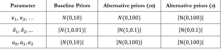
(Berger 1985).In this context, in Table 1, wepresent the baseline priors of ߢԢݏ,
[image:24.612.128.491.459.541.2]ߜԢݏ and ܽᇱݏ, as well as a set of alternative priors, which are centered at m and have standard deviations s.
Table 1: Priors
Parameter Baseline Priors Alternative priors (m) Alternative priors (s)
ߢଵ, ߢଶ, … ܰሺͲǡͳͲሻ ܰሺͲǡͳͲͲሻ ȁሺͲǡͳͲͲሻȁ
ߜଵ, ߜଶǡ ǥ ȁܰሺͳǡͲǤͲͳሻȁ ȁሺͳǡͲǤͳሻȁ ȁሺͲǡͲǤͳሻȁ
ܽǡ ܽଵǡ ܽଶ ȁܰሺͲǡͳͲሻȁ ȁሺͲǡͳͲͲሻȁ ȁሺͲǡͳͲͲሻȁ
We produced 10,000 computations under the specified alternative priors and
the calculated results – which are available upon request by the authors – were
not found to be sensitive to the alternative priors used. This clearly implies
that we can safely proceed based on these findings. For a detailed discussion
on the theoretical foundations of prior selection see, for instance, Kass and
24 The results are illustrated in Figure 1, below.
Figure 1.Time series and posterior probabilities of episodes
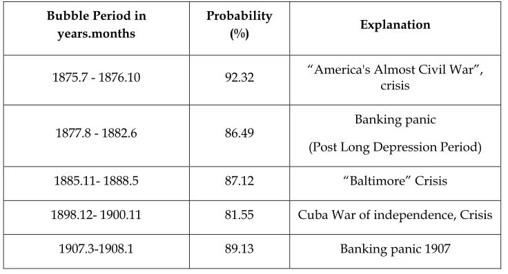
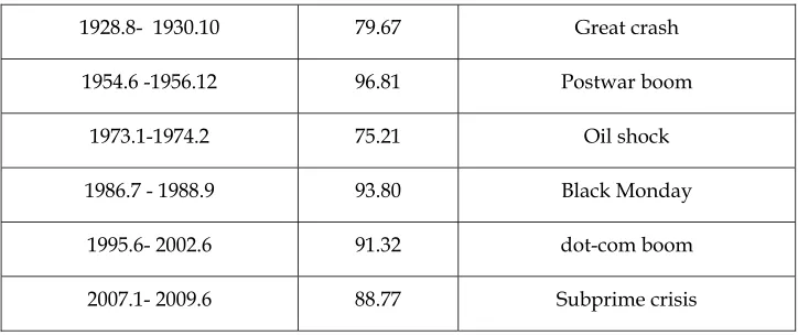
As can be seen in Figure 1 and in Table 2, the proposed specification is able to
identify eleven (11) bubble episodes or bubble formations in the S&P500 index
in the sample period (1871.1-2014.6).
Table 2.Bubble periods and Posterior Probabilities
Bubble Period in years.months
Probability
(%) Explanation
1875.7 - 1876.10 92.32 “America's Almost Civil War”,
crisis
1877.8 - 1882.6 86.49
Banking panic
(Post Long Depression Period)
1885.11- 1888.5 87.12 “Baltimore” Crisis
1898.12- 1900.11 81.55 Cuba War of independence, Crisis
[image:25.612.124.492.490.689.2]25
1928.8- 1930.10 79.67 Great crash
1954.6 -1956.12 96.81 Postwar boom
1973.1-1974.2 75.21 Oil shock
1986.7 - 1988.9 93.80 Black Monday
1995.6- 2002.6 91.32 dot-com boom
2007.1- 2009.6 88.77 Subprime crisis
In comparison to PSY, we are able to identify four (4) more bubble episodes in
[image:26.612.126.488.99.251.2]the S&P500 index and miss only one. See Table 3, below3.
Table 3:Comparison for bubble detection
Bubble Period in
years.months Bubble Explanation
Bubble detected in the present paper?
Bubble detected in PSY?
1875.7 - 1876.10 “America's Almost
Civil War”, crisis
Yes No
1885.11- 1888.5 “Baltimore” Crisis Yes No
1898.12- 1900.11 Cuba War of
independence, Crisis
Yes No
1973.1-1974.2 Oil shock Yes No
1917.08-1918.04 The 1917 Stock
Market Crash
No Yes
Another very interesting finding is that the bubbles do not have the same time
duration, in comparison to PSY. See Table 4, below.
Table 4: Comparison between bubble durations
3We would like to thank an anonymous referee for suggesting the inclusion of Tables 3 and 4,
[image:26.612.126.488.333.529.2]26
Bubble Period in years.months identified in the
present paper
Bubble Period in years.months identified inPSY
Earlier Detection of Bubbles in the present paper
compared to PSY?
How many months earlier was the bubble detected in
the present paper compared to
PSY?
1877.8 - 1882.6 1879.10-1880.4 Yes 14 months
1907.3-1908.1 1907.9-1908.2 Yes 6 months
1928.8- 1930.10 1928.11-1929.10 Yes 3 months
1954.6 -1956.12 1955.1-1956.4 Yes 7months
1986.7 - 1988.9 1986.6-1987.9 No -1months
1995.6- 2002.6 1995.11-2001.8 Yes 5months
2007.1- 2009.6 2009.2-2009.4 Yes 25months
Hence, our bubble detection mechanism seems to be more sensitive to
bubble formation.
As can be seen in Table 4,compared to PSY, the bubble episodes
thatweidentify, in general,have longer duration. This means that the proposed
specification is able to identify bubble episodes earlier, compared to PSY.
Therefore, the proposed specification could be thought of as an EWM.
For instance, if we focus on the recent US subprime crisis, the proposed
test indicates that the bubble started in January 2007 and ended in June 2009.
According to official data (CIA World Factbook, 2011), the US subprime
bubble started in December 2007, i.e. almost 10 months after ourproposed test
27 bubble, and of the one provided by the official statistics, are exactly the same.
This clearly implies that according to the proposed test, this 10-month period
coincides with the build-up of the bubble.
Analytically, the proposed specification, based on the aforementioned
dating algorithm, is capable of sufficiently answering the fundamental
question of every EWM mechanism, which is the timing of detection, while
taking into consideration the neglected non-linearities. The appropriate
timing of an ideal EWM is crucial for policy makers as the EWMs need to
signal the crisis early enough so that policy actions can be implemented in
time to be effective. The time frame required to do so depends, inter alia, on the lead-lag relationship between changing a specific macroprudential tool
and on the impact on the policy objective (CGFS 2012).
For instance, in contrast to monetary policy, where it takes at least a year
for interest rates to impact on inflation, this relationship is less well
understood for macroprudential instruments. Yet, it is likely to be at least as
long. For instance, banks have one year to comply with increased capital
requirements under the countercyclical framework of Basel III (Basel
Committee, 2010). In addition, data are reported with lags and policy makers
do not act immediately on developments but observe trends for some time
before changing policies (Bernanke 2004). This urges EWMs to start issuing
signals well before a crisis occurs as is the case with the suggested approach.
In fact, early bubble identification could substantially aid policy makers,
worldwide. The validity of this argument lies of the fact that whilst tools and
actual policies differ across countries and financial institution, the key
objective of macroprudential policies, which is the reduction of systemic risk,
remains the same(e.g. Borio 2009; Disyatat 2010). In this context, a crucial
component of the macroprudential approach based on EWMs is to address
the procyclicality of the financial system by, for example, stipulating the
accumulation of buffers in “good times” so that these can be drawn down in
28 in this regard, include countercyclical capital buffers or dynamic
provisioning. See Cukierman (2013). One key challenge for policy makers is
the identification of the different states in real time, with particular emphasis
on detecting unsustainable booms that may end up in a financial crisis.
6.
Conclusion
Despite the fact that the history of financial bubbles is rather long, only
limited attention has been paid by the scientific community to the creation of
a rigorous econometric test for the early detection of bubble formation.
Probably, one of the main reasons behind the inability of most models to
efficiently capture the formation of bubbles, is the fact that bubble formation
has inherent non-linear characteristic which are difficult to be captured using
standard econometric models.
Additionally, another equally important challenge for the econometric
detection of bubbles is the datingofbubbles’ occurance, in the sense that an
econometric test should be able to accurately date the bubble periods detected
in the sample. Accurate dating of financial bubbles could have important
policy implications, especially for central bankers and policy makers, since it
could substantially aid the implementation of policy actions that could
potentially ease the consequences of bubbles.
However, only few papers in the literature use recursive estimation
techniques for dating multiple bubble episodes. More precisely, a recent
strand in the literature, attempts to detect and date bubble episodes based on
the unit root behavior of key financial variables. In this paper, we
extendedthis strand of the literature by using ANNsin an attempt to
approximate the basic unit root specification so as to account for neglected
non-linearities.Moreover, we provided a recursive dating procedure for
bubble episodes and we applied both our bubble detection test and its dating
29 According to our findings, the proposed specification is fully capable
of capturing the bubble episodes in the time sample examined. Additionally,
the bubble periods identified are longerin comparison to PSY. More precisely,
in all common bubble episodes our proposed specification identified the
bubble, in the general case, earlier compared to PSY. In other words, our
specification could be thought ofas an EWMfor bubble formation, which in
turn could have important implications.
In brief, the early identification of bubblesis of outmost importance for
policy makers and central bankers, as we have seen. The importance of early
identification lies in the timing of implementation of specific countermeasures
that could potential prevent: a) the magnitude of a potential collapse through
regulatory interventions in the financial markets; b) the downturn effects of
bubble collapse in the economy through appropriate inflation targeting; and
c) the devastating spillover effects in the global economy through interest rate
and/or exchange rate setting.
Of course, there are still numerous issues that could serve as examples
for further investigation. For example, from a theoretical point of view, one
could explore the limit theory characteristics of the proposed approach or,
from an empirical point of view, onecould make anattempt to explore
alternative NN architectures. Clearly, future research in capturing and
30
REFERENCES
Abreu D. andBrunnermeier K. M. (2003). ”Bubbles and crashes”, Econometrica, 71(1): 173–204.
Barlevy G. (2007). "Economic theory and asset bubbles," Economic Perspectives, Federal Reserve Bank of Chicago, issue Q III, pages 44-59.
Baxa J. and Horvath R. and Vasicek B., (2013), “Time varying monetary rules and financial stress: Does financial instability matter for monetary policy?”,Journal of Financial Stability, 9(1):117-138.
Bernanke, B S (2004): "Gradualism", Remarks at an economics luncheon cosponsored by the Federal Reserve Bank of San Francisco (Seattle Branch) and the University of Washington, Seattle, 20 May 2004.
Bishop, C.M. (1995), Neural Networks for Pattern Recognition, Clarendon Press, Oxford.
Borio, C and M Drehmann (2009): "Assessing the risk of banking crises - revisited", BIS Quarterly Review, March, 29-46.
Blanchard, O. and M. Watson.(1982). “Bubbles, Rational Expectations, and Financial Markets,” in Paul Wachter (ed.) Crises in the Economicand Financial Structure. Lexington, MA: Lexington Books: 295- 315.
Brunnermeier K.M. 2009.“Deciphering the Liquidity and Credit Crunch 2007–2008”,
Journal of Economic Perspectives, 23(1):77-100.
Campbell Y.J.and Lo W. A. and MacKinlay A. C. 1997.”The Econometrics of Financial Markets”, Princeton University Press, Princeton, New Jersey.
Carlin, B. P. and Louis, T. A. (2000), Bayes and Empirical Bayes Methods for Data Analysis, Second Edition, London: Chapman & Hall.
Caruana, J (2010): "The challenge of taking macroprudential decisions: Who will press which button(s)?". Speech at the 13th Annual International Banking Conference, Federal Reserve Bank of Chicago, in cooperation with the International Monetary Fund, Chicago, 24 September 2010.
31
Committee on the Global Financial System (CGFS) (2012): "Operationalising the selection and application of macroprudentialinstruments", CGFS Publications No. 48.
Cucierman A., (2013), “Monetary policy and Institutions before, during and after the global financial crisis”, Journal of Financial Stability, 9 (3): 373-384.
DeMarzo M. P. and Kaniel R. and Kremer I., 2008. "Relative Wealth Concerns and Financial Bubbles," Review of Financial Studies, 21(1):19-50.
Dezbakhsh, H. and A.Demirguc-Kunt.(1990). “On the Presence of Speculative Bubbles in Stock Prices,” The Journal of Financial andQuantitative Analysis,25:101-112.
Diba, B. and H. Grossman. (1988a). “The Theory of Rational Bubbles in Stock Prices,” The Economic Journal, 98(September): 746- 54.
Diba, B. and H.l Grossman.(1988b).”Explosive Rational Bubbles in Stock Prices?”American Economic Review,78(June): 520-30.
DiCiccio, T. J., Kass, R. E., Raftery, A. and Wasserman, L. (1997).“Computing Bayes factors by combining simulation and asymptotic approximation”, Journal of American Statistical.Association, 92, 903-915.
Disyatat P., (2010), “Inflation targeting, asset prices, and financial Imbalances: Contextualizing the Debate”, Journal of Financial Stability, 6(3):145-155.
Dufwenberg, Martin, Tobias Lindqvist, and Evan Moore. 2005. "Bubbles and Experience: An Experiment." American Economic Review, 95(5): 1731-1737.
Evans,G.(1991).“PitfallsinTestingforExplosiveBubblesinAssetPrices,”AmericanEconomicRevi ew31(September): 922-30.
Fama, E. (1965).“The Behavior of Stock Market Prices", Journal of Business, 38: 34–105.
Flavin, M. (1983). “Excess Volatility in the Financial Markets: A Reassessment of the Empirical Evidence,” Journal of Political Economy, 91(December): 929-956.
Flood P. R and Hodrick J. R. (1990). ”On testing for speculative bubbles”, Journal of Economic Perspectives, 4(2):85-101.
Flood, R. and R.Hodrick. (1986). “Asset Price Volatility, Bubbles and Process Switching,”
Journal of Finance,41(September): 831-42.
32
Granger, C and M Machina (2006): "Forecasting and Decision Theory," In Elliott, G, C Granger and A Timmermann (Eds.), Handbook of Economic Forecasting, Elsevier.
Greenwood, R. and Nagel, S. (2009). "Inexperienced investors and bubbles," Journal of Financial Economics, 93(2):239-258.
Hall, S. and M. Sola. (1993). “Testing for Collapsing Bubbles: An Endogenous Switching ADF Test,” Discussion paper 15-93, London Business School.
Hall, S., Z.Psaradakis, and M. Sola. (1999). “Detecting Periodically Collapsing Bubbles: A Markov-Switching Unit Root Test,” Journal of Applied Econometrics, 14: 143-154.
Haruvy E. and Noussair N. C. (2006), “The Effect of Short Selling on Bubbles and Crashes in Experimental Spot Asset Markets’, Journal of Finance 61(3): 1119-1157.
Haykin, S. (1999), Neural Networks, Prentice-Hall, New Jersey.
Homm U. and Breitung J., (2012). "Testing for Speculative Bubbles in Stock Markets: A Comparison of Alternative Methods," Journal of Financial Econometrics, 10(1): 198-231.
Hong H. and Scheinkman J. and Xiong W, (2006). "Asset Float and Speculative Bubbles,"
Journal of Finance, 61(3): 1073-1117.
Hornik, K. (1991). “Approximation capabilities of multilayer feedforward networks”,
Neural Networks, 4(2):251-257.
Hornik, K., Stinchcombe, M., White, H. (1989).“Multilayer feedforward networks are universal approximators”, Neural Networks 2, 359–366.
Hornik, K., Stinchcombe, M., White, H. (1990).“Universal approximation of an unknown mapping and its derivatives using multilayer feedforward networks”, Neural Networks 3, 551–560.
Kapetanios G., Shin Y. and Snell A.(2003). “Testing for a unit root in the nonlinear STAR framework”, Journal of Econometrics, 112 (2): 359-379.
Keynes, J. M, (1936). “The General Theory of Employment, Interest and Money”, London: Macmillan.
Kindleberger, C. P., and Aliber, R. Z. (2005), “Manias, Panics and Crashes; A History of Financial Crises”, Hoboken, New Jersey: John Wiley and Sons, Inc.
33
Kuan, C.M., White, H. (1994). “Artificial neural networks: An econometric perspective”,
Econometric Reviews, 13, 1–91.
Lawrence, M, P Goodwin, M O'Connor and D Onkal (2006): "Judgmental forecasting: A review of progress over the last 25years", International Journal of Forecasting, 22, 493-518.
LeRoy, S, and R.Porter(1981). “The Present-Value Relation: Tests based on Implied Variance Bounds,” Econometrica,49(May): 555- 574.
Luukkonen, R and Saikkonen, P. and Teriisvirta, T. 1988.“Testing linearity against smooth transition autoregressive models”, Biometrika 75, 491-99.
Mankiw, N. G, D.Romer, and M. Shapiro. (1985). “An Unbiased Reexamination of Stock Market Volatility,”Journal of Finance, 40(July): 677-687.
Önkal, D, M E Thomson and A A C Pollock (2002): "Judgmental forecasting", inClements, M P and Hendry, D F (eds), A companion to economic forecasting, Blackwell Publishers, Malden and Oxford.
Pesaran, M H and S Skouras (2002): "Decision-based methods for forecast evaluation". In: Clements, M P and D F Hendry (Eds.), A Companion to Economic Forecasting, Blackwell, Malden and Oxford.
Phillips P.C.B. and Shi S. and Yu J., (2014). "Specification Sensitivity in Right-Tailed Unit Root Testing for Explosive Behaviour," Oxford Bulletin of Economics and Statistics, 76(3):15-333.
Phillips P.C.B. and Wu Y. and Yu J., (2011b). "Explosive Behavior in the 1990s Nasdaq: When Did Exuberance Escalate Asset Values?",International Economic Review, 52(1): 201-226.
Phillips P.C.B.and Yu J, (2011c). "Dating the timeline of financial bubbles during the subprime crisis," Quantitative Economics, 2(3):455-491.
Phillips, P. C. B., Shi, S. and Yu, J. (2011a).Testing for Multiple Bubbles, Singapore Management University, Working Papers No. 09-2011.
Phillips, P. C. B., Shi, S. and Yu, J. (2013).“Testing for Multiple Bubbles 1- Historical episodes of Exuberance and Collapse in the S&P 500m Singapore Management University, Working Papers No4-2013.
34
Phillips P. C. B., Shi, Shuping and Yu, Jun (2105b), TESTING FOR MULTIPLE BUBBLES: HISTORICAL EPISODES OF EXUBERANCE AND COLLAPSE IN THE S&P 500, International Economic Review, Vol. 56, No 4, 1043-1078.
Robert, C. P. (2001), The Bayesian Choice, Second Edition, New York: Springer-Verlag.
Rudin, W. (1976). “Principles of Mathematical Analysis”, McGraw-Hill, New York, International Edition.
Sanger, T.D. (1989), Optimal Unsupervised learning in a Single Layer Linear Feedforward Neural Network, Neural Networks, 2: 495-479.
Scheinkman J. and Xiong W.(2002). "Overconfidence, Short-Sale Constraints and Bubbles," Princeton Economic Theory Working Papers 98734966f1c1a57373801367f, David K. Levine.
Shiller, R. (1981). “Do Stock Prices Move Too Much to be Justified by Subsequent Changes in Dividends?” American Economic Review71(June): 421-436.
Smith, A. F. M. and Gelfand, A. E. (1992), Bayesian statistics without tears: A sampling– resampling perspective,American Statistician 46, 84–88
Temin P. and Voth H-J., 2004. "Riding the South Sea Bubble," American Economic Review, 94(5):1654-1668.
Tierney L. 1994. “Markov Chains for exploring posterior distributions”, Annals of Statistics, 22(4):1701-1728.
Tirole, J. (1982). “On the Possibility of Speculation under Rational Expectations,”
Econometrica,50: 1163-1182.
Van Norden, S. and R.Vigfusson. (1998). “Avoiding the Pitfalls: Can Regime-Switching Tests Reliably Detect Bubbles?” Studies in NonlinearDynamics and Econometrics,3:1-22.
Van Norden, S. (1996). “Regime Switching as a Test for Exchange Rate Bubbles,” Journal of Applied Econometrics,11(July): 219-51.
Wasserman, L. (2004), All of Statistics: A Concise Course in Statistical Inference, New York: Springer-Verlag.
35
White W. R., (2008), “Past financial crises, the current financial turmoil and the need for a new macrofinancial stability theory”, Journal of Financial Stability, 4(4):307-312.
Wu, G and Z Xiao. (2002). “Are there Speculative Bubbles in Stock Markets? Evidence from an Alternative Approach,” working paper, Michigan Business School.
Wu, Y., (1997), "Rational Bubbles in the Stock Market: Accounting for the U.S. Stock-Price Volatility," Economic Inquiry, 35(2):309-319.