Financial time series representation using multiresolution important point retrieval method

106

FINANCIAL TIME SERIES REPRESENTATION USING

MULTIRESOLUTION IMPORTANT POINT RETRIEVAL

METHOD

Chaliaw Phetkingl,Mohd Noor Md. Sap2,Ali Selamat2

I.2Faculty of Computer Science and Information System

Universiti Teknologi Malaysia,lohor, Malaysia

[email protected],2{mohdnoor,aseJamat }@utm.my

Abstract: Financial time series analysis usually conducts by determining the series important

points. These important points which are the peaks and the dips indicate the affecting of some

important factors or events which are available both internal factors and external factors. The

peak and the dip points of the series may appear frequently in multiresolution over time.

However, to manipulate financial time series, researchers usually decrease this complexity of

time series in their techniques. Cons~quently,transforming the time series into another easily

understanding representation is usually considered as an appropriate approach. Inthis paper, we propose a multiresolution important point retrieval method for financial time series

representation. The idea of the method is based on finding the most important points in

multiresolution. These retrieved important points are recorded in each resolution. The

collected important points are used to construct the TS-binary search tree. From the TS-binary

search tree, the application of time series segmentation is conducted. The experimental results

show that the TS-binary search tree representation for financial time series exhibits different

performance in different number of cutting points, however, in the empirical results, the

number of cutting points which are larger than 12 points show the better results.

Keywords: Financial time series, Multiresolution , TS-binary search tree, SB-binary search

tree, Segmentation

1. INTRODUCTION

Time series analysis is become one of the most popular data mining tasks and is widely

applied in many research areas; for example, economics, finance, medicine, chemistry,

bioinformatics, etc. For financial time series, the data are generated from the complex and

dynamic system with noisy, non-stationary and chaotic data series [I]. Financial data such as

stock prices or currency exchanges are discrete time series of prices data. A financial time

series demonstrates its movement in a fluctuant way due to some important factors or events

which are available both internal factors (e.g. company news) and external factors (e.g.

politics, economic growth). These important factors usually reflect to stock prices or

exchange rates directly.

Financial time series researches usually relate to following tasks; pattern matching[3],

segmentation[4], dimensionality reduction[5], c1ustering[6], and forecasting[7]. As with all

time series data mining problems, the key to effective and scalable algorithms is choosing a

suitable representation of the data [2]. Many researchers propose the representation

techniques of time series data as found in reference [2],[8],[9],[ 10]. Authors in [8] propose an

Extended Symbolic Aggregate ApproXimation(ESAX) which is a symbolic representation of

financial time series. ESAX was adapted from the original SAX[2]. In reference[9], the

author presents a generalized model in financial time series by the utilizing of turning points

in financial data. Turning points can be considered as the important points in a study done by

Fu et al. [10].

In the study of Fu et al. [10], they propose a financial time series representation based

on the Perceptually Important Points(PIPs)[lI] which are mapped to SB-Tree data

structure. These PIPs are collected by measuring the distance between the series

points and their trend. The point that has the largest distance is chosen. Alternatively,

the important points exist in the series usually occur in as both the peak points and the

dip points with the equivalent importance priority. Thus, it is better to collect both the

most peak point and the most dip point in the same time or in the same iteration.

In this paper, we introduce a TS-binary search tree for financial time series data based on

a Multiresolution ImportaNt pOits Retrieval (MINOR) method. MINOR is used for collecting

the most important points (MIPs) which comprises of the most peak (MP) point and the most

dip (MD) point. The MIPs are collected in multiresolution views and used for constructing the

TS-binary search tree. The financial time series segmentation is conducted as an

implementation.

This paper is organized as following. Section 11, we introduce the MINOR method.

Section JJl the TS-binary search tree for financial time series representation is proposed.

Section IV, an example of trend based financial time series segmentation is conducted. The

last section, the conclusion and recommendation for future works are described.

2. RETRIEVALS OF THE MOST IMPORTANT POINTS

In this section, the retrieval of the most important points of financial time series is

focused. Firstly, the multiresolution important point retrieval method is conducted, and the

second section, the method of finding the most important points is described.

2.1 MINOR method

Given time series S= {Sj, S2, S3, ... ,sm}, where m is the length of time series. First, finding

the global trend of the time series sequence is processed by drawing a trend line which

connects the first point and the last point of the time series. Next, the MIPs which comprises

of MP and MD points are recorded. To retrieve the MP and the MD points from the time

series, we apply the Finding the Most Important Points (FiMIP) method. Consequently, the

MP and MD points are used as cutting points, then, the time series is divided into three

subsequences. For each subsequence, starting from the first subsequence, finding the trend of

the subsequence is conducted and then finding MP and MD points of the subsequences are

determined and recorded.

The algorithm is performed recursively until the final condition is met. The final condition

is the length of final subsequences which is designed by user. However, the smallest length of

a subsequence that can be used as the final condition is 3. The pseudo code of the MINOR

method is depicted in figure I.

Function MINOR(S,cond) Input sequence S[ I..m] Integer cond

Output list MIPL,sl Begin

Repeat while length(S)>~cond MIP~FiMIP(S.cond) Add MIP to MIPList

Divide segment S into S I, S2 and S3 at MIP Recursively call to MINOR for all S I,S2,S3 End

End

Return MIPL,sl End

Figure I Pseudo code for MINOR method

2.2 FiMIP method

Given a time series segment S = { 51,52, ""Sm-I, sm}, the algorithm of FiMIP can be

illustrated as following.

MIP is a set of the most important points obtained from a sequence. Two kinds of points

are collected; MP and MD points. Each pair of MP and MD is retrieved from a sequence in

iteration. The MP point is the point that has the largest distance away up from the trend line of

the sequence and the MD point is the point that has the largest distance away down from the

trend line of the sequence. Measuring of the distance can be determined by various methods;

for example, Euclidean distance(ED), perpendicular distance (PD), and vertical distance

(VD).

Actually, the distance value is positive for MP point and negative for MD point. In

particular, in this paper vertical distance measurement is selected because of the better results

in capturing of the highly fluctuated points [10]. The illustration of the method is depicted in

figure 2.

f

f""'"

p'"

1

d2

s2(x2,y2)

sm -l(xm -1,ym -1)

dm-1

b

,sm -l'(xm -l',ym -11

s... sm(xm,ym)

Figure 2 VD height measuring

As can be seen, figure 2 illustrates a vertical distance measurement. The method is started

from making a trend line connecting between the first and the last points, we can see as the

lineSISm in figure 2. From the trend line, we can see that peak points appear up higher than

the lineSISm, and conversely, the dip points appear lower down from the lineSISm' Different

points correspondingly give different distance far away from the lineSISm'Every point around

the line SISm must be measured its distance. In figure 2., for example, the point Sz appears

110

lower than the line SJSmand the pointSm-Jappear higher than the lineS.Sm' In case of the point

S2, the distance d₂is measured. As can be seen above, d₂is a straight line connecting between

S2 andsz', thus d2is a distance betweenS2 andS2'orYrYz' or we can say d2is a YO ofS2. For

the point Sm.j, we can find its YO in similar way. In general, the distance of the ith point is

Yi-Y/can be calculated as equation 1.

d,=Y, -Y,'

wherex, andy,are the coordinate of theithpoint and 1OS;iOS;m.Y" Yeare the value of the time series at the first pointX.Iand the end pointXerespectively.

In figure 2, supposedly, if YO ofs2is the smallest value and if YO ofsm _, is the largest

value, thus, we can recordS2and its YO as MO point and recordSm-J and its YO as MP point.

t

[

L

(a) (b)

Figure 3 All points are lower than the trend line(a) and all points are lower than the trend line(b).

Nevertheless, there are other two special cases of FiMIP method. These two special cases

are depicted in figure 3 and figure 4.

Finding the MPO points in other two cases, their calculations h,we a little bit of

difference. In figure 3(a), all points appear as dip points; the MP point is not available. Thus,

in this case we can record MO point information but MP point cannot be recorded, so it is set

to be NULL. Similarly, in figure 3(b), all points appear as peak points, thus, the MP point is

recorded while MO point is set to be NULL.

111

3. TS-BINARY SEARCH TREE REPRESENTAnON

TS(Time Series)-binary search tree is designed as a variety of binary search tree with

additionally special nodes and their arcs information while the binary search tree properties

are kept. As can be seen, in binary search tree, ifxis a node with key value key[x] and it is

not the root of the tree, then the node can have a left child (denoted by left[x]), a right child

(right[x]) and a parent (p[x]). Every node of a tree is constructed under the following binary

search tree properties:

(I) for allnodesyin left subtree ofx,key[y] <key[x]

(2) 'for all nodesyin right subtree ofx,key[y]>key[x]

The additional nodes in TS-binary search tree are the two special nodes; one is the first

element of the time series, which is placed at the first node of the tree, and the other one is the

last element of the time series which is placed as the right child of the first node. These two

nodes, their iterations and their distances equal to zero.

To construct the next node of the TS-binary search tree, the founded MIPs are adopted.

The first used point is the peak point which is a member of the pair of the peak and the dip

points, however, if the peak is not available the second point-the dip point is determined.

The construction of the tree is performed recursively. From the root node, let root is the

pointer points to the root, and newNode is the node, which is formed by the current MIPs.

For more detail, following is an example of the representation demonstration with the

ten-point time series data. The data is transformed into the range of 0 and I. The graphical

illustration of the time series is shown in figure 4.

'1

0.9 /: \ 0.8 i: \

I ' \

07 / : \

i

0.6

0.5

0.4

0.3 /

I

0.2j

I 0.1

112

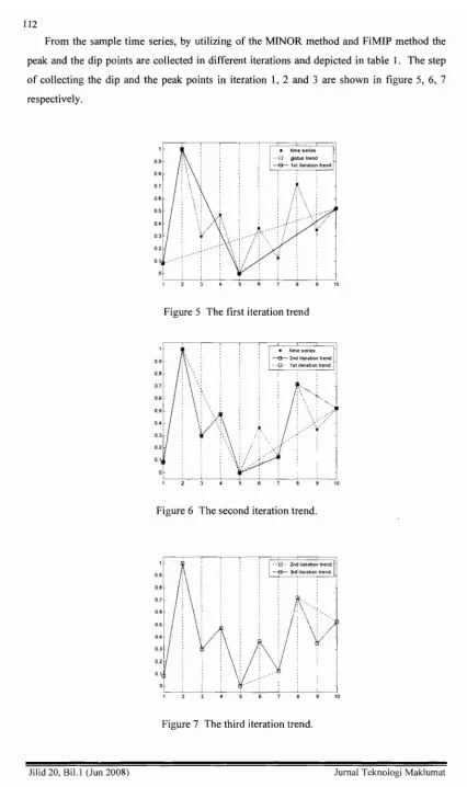
From the sample time series, by utilizing of the MINOR method and FiMIP method the

peak and the dip points are collected in different iterations and depicted in table I. The step

of collecting the dip and the peak points in iteration I, 2 and 3 are shown in figure 5, 6,7

respectively.

'~

0.9 : \

0.8 i \

071 . \

0.6

0.1

~

- - 0 -global trend -a---1st iteration trend

10

Figure 5 The first iteration trend

0.9

o.a

0.1

• time series

-a----2nd iteration trend - - E} - 151 Iteration trend

~'" :

I~\ -.~_

\ : "'..,

\: ~;)

\....:-->/

.-

",

10

Figure 6 The second iteration trend.

0.9

o.a

0.7

0.1

§ d it...Ioon t<end -e---3rd iteration trend

;\-.

/

\

:yN::/:\V

.

/

. . .

. .

10

.Iilid 20. BiJ.l (.Tun 2008)

Figure 7 The third iteration trend .

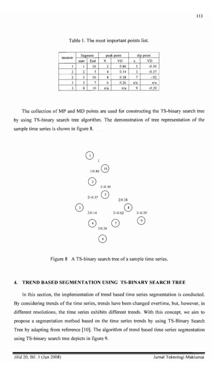
Table 1. The most important points list.

iteration Segment peak point dip point

star! End X vo x vo

1 I 10 2 0.86 5 -0.30 2 2 5 4 0.14 3 -0.37

2 5 10 8 0.38 7 -.02 3 5 7 6 0.26 n/a n/a

3 8 10 n/a n/a 9 -0.20

The collection of MP and MD points are used for constructing the TS-binary search tree

by using TS-binary search tree algorithm. The demonstration of tree representation of the

sample time series is shown in figure 8.

8

G

1/0.86

Q

1/-0.30

2/-0.37

0

2/038

0

8

8

G

G

G

Figure 8 A TS-binary search tree of a sample time series.

4. TREND BASED SEGMENTATION USING TS-BINARY SEARCH TREE

In this section, the implementation of trend based time series segmentation is conducted.

By considering trends of the time series, trends have been changed overtime, but, however, in

different resolutions, the time series exhibits different trends. With this concept, we aim to

propose a segmentation method based on the time series trends by using TS-Binary Search

Tree by adapting from reference [10]. The algorithm of trend based time series segmentation

using TS-binary search tree depicts in figure 9.

The algorithm firstly considers the MIP in the lowest resolution by accessing the tree

from root. The first-two nodes are retrieved from the first and the last points of the time

series. Consequently, accessing the next node is determined by the node iteration and its YD.

From the time series in figure 4 and its tree in figure 8, the next node to access is the node

x=2 this shows the result of segmentation in figure 9(a). Next,the node x=5 is retrieved since

its iteration is 1 and it has a largest VD after previous node, this makes the time series is

segmented into three segments as shown in figure 9(b).

The next accessing node is considered with the node with iteration 2, but, in this iteration

there are 4 choices, the largest VD node should be retrieved first, thus, node x=8 is retrieved.

With the 3 accessed nodes, the time series is segmented into 3 segments as shown in figure

9(c). By considering in the similar way, the following nodes should be retrieved are node x

equals to 3, 4, 7, 9, and 6 respectively.

(a)

:Q'.("

J

(b)

.:i

I

I

"l·,···/1 \ ! .. 'I \ I

::;)' " 1 /

1

::,/ '. J ,,/ j

'.LL .

~~J

Figure 9 A sample time series with 1 cutting point(a), 2 cutting points(b) and 3 cutting points(c).

S. EXPERIMENTAL RESULTS

In this section, we experiment the segmentation algorithm with 2725 data points of

closing prices of Hang Seng Index (HSI) since January 2, 1997 until December 31,2007. The

results of segmentation are reported in different number of segments and comparing between

the results done by our method and the results done by the method proposed in reference [10].

The segmentation results of our experiments are done by using our proposed method and

comparing to the SB-Tree based method [10]. The comparisons are conducted by the

segmentations in di fferent number of 3, 4, 6, 8, 10, 12, 14, 16, 18, and20cutting points.

The performance of segmentation is measured by the root mean square errors

(RMSE). The RMSE can becalculated from the distances between the original time

series and its segment trends. Table

2

10demonstrates the comparison of those two methods.

(a)

T

--T

,

j

_~_~J

'000 '500 2000 2500 3000

(b)

06

T

O.

j

J

.000 '500 2000 2500 3000

Figure 10 Segmentation of HSJ index using: SB-Tree based segmentation in 3 and 7

segments respectively (a),(b) , and TS-Binary Search Tree based segmentation in3and7

segments respectively(c),(d).

(c)

'r---3000

(d)

o.

06

1000 1500 2000 2500 3000

Figure 10 Segmentation of HSI index using: SB-Tree based segmentation in 3 and 7

segments respectively (a),(b) , and TS-Binary Search Tree based segmentation in 3 and 7

segments respectively(c),(d). (Cont'.)

Table 2. Numbers of cutting points and the errors

No. of cutting RMSE

points TS-BS tree SB- tree

3 0.1263 0.1263

4 0.1714 0.1325

6 0.1081 0.0678

8 0.0677 0.0647

10 0.0648 0.0770

12 0.0633 0.0881

14 0.0636 0.0849

16 0.0635 0.0688

18 0.0644 0.0675

20 0.0630 0.0650

1--

RMSE ,-'-'-\

0.12 \ ,

oO~Lj\~/""'"

---a~ ,

3 .. 6 5 10 12 1. 16 18 20

number of cutting points

Figure I I Performance comparison of segmentation based on TS-binary search tree method

and SB-binary search tree method

As can be seen in table 2 and figure II, the RMSE of the segmentation the errors show

sharp peaks at 4 cutting points on both two methods and dramatic falls until number of cutting

points are 8. At the 8-cutting points, the graph show almost the same error values. However,

from the 8 cutting points, SB-tree based methods gradually increases until number of cutting

points is 12, then, the graph slightly declines and remain stable. While the errors of SB-tree

based method between 8 to 12 cutting points, the graph show a remain constant and less

errors comparing to the SB-tree based method.

6. CONCLUSION

In this paper, we have proposed a method for financial time series representation based on

the most important points retrieval method. The idea of the method is based on finding the

most important points in multiresolution. These retrieved important points are recorded in

each resolution. The collected important points are used to construct the TS-binary search

tree. From the TS-binary search tree, the application of time series segmentation is conducted.

Our experiments have been tested on the real stock market time series.

The proposed method shows that the performance of the method is better when using the

segmentation with number of segments more than 6 cutting points and the results show very

poor performance when using the cutting points less than or equal to 6. Future works the

method should be applied in other dataset and with different size of the dataset.

REFERENCES

[I] Peters E.E., Chaos and order in the capital markets. John Willey&Sons 1996.

[2] Lin 1., Keogh E., Lonardi S., Chiu B. A Symbolie Representation of Time Series, with

Implications for Streaming Algorithms. In proceedings of the 8th ACM SIGMOD

Workshop on Research Issues in Data Mining and Knowledge Discovery. (2003).

[3] FuT-C., Chung F-L., Luk R., Ng C-M., Stock time series pattern matching:

Template-based vs. rule-Template-based approaches. Engineering Applications of Artificial Intelligence 20,

2007, pp.347-364.

[4] Chung F-L, FuT-C, Ng V., Luk R.W.P., An Evolutionary Approach to Pattern-Based

Time Series Segmentation. IEEE Transactions on Evolutionary Computation 8, 5.

October 2004, pp. 471-489.

[5] Wang Q., Megalooikonomou, V. A dimensionality reduction technique for efficient

time series similarity analysis. Information Systems 33, March 2008. pp.115-132.

[6] Pattarin F.. Paterlini, S., Minerva, T. Clustering financial time series: an application to

mutual funds style analysis. Computational Statistics & Data Analysis 47, 2, September

2004, pp.353-372.

[7] Hueng C.J., McDonald, J.B., Forecasting asymmetries in aggregate stock market

returns: Evidence from conditional skewness. Journal of Empirical Finance 12,5,

December 2005,pp.666-685.

[8] Battuguldur Lkhagva, Yu Suzuki, Kyoji Kawagoe: New Time Series Data

Representation ESAX for Financial Applications. ICDE Workshops 2006.

[9] Bao D. A generalized model for financial time series representation and prediction.

Applied Intelligence, DOl: 10.1 007/s I0489-007-01 04-9 .

[ltD] Fu T-C.." Chung F-L., Luk R..'and N(g·C-M., Representing financial time series based on data point iimpurtance., Enqgineerirlg Applications <of Artificial IntclligenceVolume 21,

2,March2!008, pp.277-300..

lll] Chung, F-L., Fu, T-C., Luk, iR..,1'Ng, V. Flexible time sories ¥Idem matching based on

perceptually important poi1U5. In: Internationall Jiliint Conference on Arti ficial

Intelligence Workshop on Learning from Tempordll and Spatial Data, pp.1-7.