Fat Tails and Spurious Estimation of Consumption Based Asset Pricing Models

Munich Personal RePEc Archive

Fat Tails and Spurious Estimation of

Consumption-Based Asset Pricing

Models

Toda, Alexis Akira and Walsh, Kieran James

University of California, San Diego, Darden School of Business,

University of Virginia

17 November 2016

Online at

https://mpra.ub.uni-muenchen.de/78980/

Fat Tails and Spurious Estimation of

Consumption-Based Asset Pricing Models

∗

Alexis Akira Toda

Kieran James Walsh

November 17, 2016

Abstract

The standard generalized method of moments (GMM) estimation of Euler equations in heterogeneous-agent consumption-based asset pricing models is inconsistent under fat tails because the GMM criterion is asymp-totically random. To illustrate this, we generate asset returns and con-sumption data from an incomplete-market dynamic general equilibrium model that is analytically solvable and exhibits power laws in consump-tion. Monte Carlo experiments suggest that the standard GMM esti-mation is inconsistent and susceptible to Type II errors (incorrect non-rejection of false models). Estimating an overidentified model by dividing agents into age cohorts appears to mitigate Type I and II errors.

Keywords: consumption-based CAPM, generalized method of mo-ments, heterogeneous-agent model, power law

JEL codes: C58, D31, D52, D58, G12

1

Introduction

It is well-known that the representative-agent, consumption-based capital asset pricing model (CCAPM) of Lucas (1978) and Breeden (1979) requires a relative risk aversion coefficient on the order of 10 to 100 in order to explain the historical equity premium, at least in the basic, frictionless case with additively separa-ble, constant relative risk aversion (CRRA) preferences.1 _{To explain asset prices}

with a lower risk aversion parameter, many researchers have considered the pos-sibility of market incompleteness and estimated and testedheterogeneous-agent

∗_{We thank Bertille Antoine, Brendan Beare, Chris Carroll, Russell Davidson, Lynda}

Kha-laf, Yixiao Sun, and seminar participants at Australian School of Business, Universit´e Laval, UCSD, Yale, the 17th ICMAIF at the University of Crete, and the CIREQ Conference on Financial Econometrics for comments and feedback. We especially thank two anonymous referees for suggestions that significantly improved the paper.

†_{Department of Economics, University of California San Diego. 9500 Gilman Dr, La Jolla,}

CA 92130. Email: [email protected]

‡_{Darden School of Business, University of Virginia. 100 Darden Blvd, Charlottesville, VA}

22903. Email: [email protected]

1

models2_{using household consumption data such as the Consumer Expenditure}

Survey (CEX).

In a recent paper (Toda and Walsh, 2015), we document that the cross-sectional distributions of U.S. household consumption and its growth rate ex-hibit fat tails. The power law exponent α > 0 is approximately four both in the upper and lower tails.3 _{If this is the case, the cross-sectional moments of}

consumption and its growth rate, Et[cηit] and Et[(cit/ci,t−1)η], are infinite when

the moment order ηexceeds the power law exponentαin absolute value. Such nonexistence of moments renders the generalized method of moments (GMM) estimation of aggregated household Euler equations inconsistent due to lack of identification: even if the model is correctly specified, nonexistent moments aid in zeroing the GMM criterion at untrue parameters (a Type I error). Further-more, our bootstrap studies suggest that the fat tails in consumption mechan-ically set the pricing error to zero, even when the model is incorrect (a Type II error). As we show in Section 2.2, the problem is that when the moment conditions contain nonexistent cross-sectional moments, the criterion function becomes asymptotically random. The implication is that GMM estimation may find a spurious criterion minimum due to randomness rather than to the truth of the model.

As a remedy, Toda and Walsh (2015) propose an alternative estimation approach (age cohort GMM) that divides households into age groups in order to mitigate the fat tail problem. This approach is motivated by the finding in Battistin et al. (2009) that,within age cohorts, the empirical cross-sectional distribution of consumption is approximately lognormal, which is thin-tailed.4

However, the analysis of Toda and Walsh (2015) is only suggestive since, with actual consumption data, we know neither the true data generating process nor whether the asset pricing model is a good description of reality.

In this paper, we conduct a Monte Carlo study using artificial asset re-turns and consumption data.5 The goal is to assess the robustness (or non-robustness) of estimation/testing of heterogeneous-agent asset pricing models when the cross-sectional consumption distribution exhibits fat tails and the models may be true or false. Compared to the representative-agent setting, a simulation study of a heterogeneous-agent model is challenging for two reasons. First, solving a heterogeneous-agent asset pricing model is much more

com-2

See Mankiw (1986), Constantinides and Duffie (1996), Heaton and Lucas (1996), Saito (1998), Krebs and Wilson (2004), Storesletten et al. (2007), Krueger and Lustig (2010), Gu-venen (2009), and Toda (2015) for theoretical/numerical works and Brav et al. (2002), Cogley (2002), Vissing-Jørgensen (2002), Balduzzi and Yao (2007), Krueger et al. (2008), Kocher-lakota and Pistaferri (2009), Basu et al. (2011), Constantinides and Ghosh (2014), and Se-menov (2016) for empirical works. See Ludvigson (2013) for a review on testing CCAPM.

3

A nonnegative random variableXis said to beParetian_{(obey the power law in the upper}

tail) if Pr(X > x) =Ax−α_{(1 +o(1)) asx→ ∞for someA, α >0. It obeys the power law in}

the lower tail if 1/Xis Paretian, so Pr(X < x) =Bxβ_{(1 +o(1)) asx→0 for someB, β >0.}

α, β >0 are called power law exponents. See Resnick (2008) for an authoritative textbook treatment of extreme value theory and Gabaix (2009) for a review of empirical power laws as well as some generative mechanisms.

4

Battistin et al. (2009) document the lognormality in consumption using U.S. and U.K. data. Brzozowski et al. (2010) obtain similar results with Canadian data.

5

plicated than solving a representative-agent one: heterogeneous-agent models rarely have closed-form solutions, and one must thus usually solve them numer-ically as in Krusell and Smith (1998). Solving even two agent, two asset infinite horizon general equilibrium models often entails substantial computational bur-den (Guvenen, 2009). Second, since our aim is to study the implications of fat tails for GMM estimation, the cross-sectional distribution of consumption must have fat tails. But, numerical techniques do not let us, with certainty, identify or characterize fat tails in heterogeneous-agent models.

The incomplete-market dynamic general equilibrium model of Toda (2014) overcomes both difficulties: it is analytically solvable and computationally tractable, and the model’s cross-sectional consumption distribution obeys the power law in both the upper and lower tails with known power law exponents. Although in the literature there exist heterogeneous-agent models that are analytically solvable and exhibit fat tails, such as Benhabib et al. (2011, 2016), these models do not feature aggregate shocks and therefore cannot be applied to the study of asset prices. The Toda (2014) model, on the other hand, allows for an arbitrary Markov process for the aggregate shocks. Therefore, this model is well-suited as a laboratory for examining financial Euler equation estimation in the presence of fat tails in the cross-sectional distribution of consumption.

Using the incomplete-market general equilibrium model as our laboratory, we conduct two sets of experiments. First, we estimate the relative risk aver-sion coefficient both by standard GMM and by age cohort GMM using the simulated consumption and asset returns data from the model. We find that standard GMM over-rejects the correct risk aversion coefficient and that the GMM estimator has a large mean squared error. In part, this is because in many simulations, the GMM criterion has multiple troughs, one near the true param-eter and another at a random location, which is frequently the global minimum. The risk aversion estimate is often well above 10 (in the moment nonexistence range) and, in these instances, associated with a zero equity premium pricing error. Thus, the fat tails sometimes aid in over-fitting, even though on average standard GMM over-rejects the correct model. Age cohort GMM, in contrast, provides more accurate risk aversion estimates and does not over-reject the true model/parameter.

Second, we repeat our analysis but with incorrect, random asset returns. Standard GMM quite often fails to reject the model even though it is false. In these cases of over-fitting, risk aversion estimates are upwardly biased high into the moment nonexistence range. Oddly, the histogram of equity premium pricing errors across simulations is bimodal, with spurious mass at zero. The age cohort method, on the other hand, removes the spurious pricing error peak at zero. While some of these findings seem odd, they closely mirror the empirical findings of Toda and Walsh (2015).

GMM.

Finally, using a representative-agent asset pricing model as an example, we provide a simple explanation for the bimodal pricing error histograms and the Type II errors. The idea is that since the sample moment condition involves negative powers of consumption growth, when the power is a large negative value (corresponding to high risk aversion), the sample moment condition is dominated by the two largest terms in absolute value (corresponding to the two smallest consumption growth observations). Therefore as long as these two terms have opposite signs, regardless of whether the model is true or false, we can always set the sample moment to zero at some high risk aversion parameter. Indeed, estimating a representative-agent model with the incorrect asset returns (so the model is false by construction), we get bimodal pricing errors and Type II errors, driven by high risk aversion. This explanation offers a simple remedy: estimating an overidentified model (with consumption powers in each moment condition) is likely to mitigate the Type II errors since the spurious estimators differ across equations. The age cohort method is an example of this remedy.

Our paper is related to two strands of literature. The first is the literature on model estimation under fat tails. In an asset pricing setting, Kocherlakota (1997) tests the standard representative-agent CCAPM with fat-tailed pricing errors using subsampling. Here the fat tails appear in the time series, whereas in our analysis they appear in the cross-section of consumption. While he tests the model using actual data, our focus is the estimation from simulated data, for which we know by construction both the data generating process and whether the model is true or false.6 _{Beaulieu et al. (2010) test the Fama-French}

multi-factor CAPM with fat-tailed asset returns. Although not in a financial context, Geweke (2001) describes the limitations of the constant relative risk aversion (CRRA) utility function: expected utility may not exist when the distribu-tion of consumpdistribu-tion is fat-tailed. In the GARCH setting, when error moments become infinite between 2 and 4, the convergence rate of quasi-maximum like-lihood (QML) estimation falls belown1/2 _{(Berkes and Horv´ath, 2003), and the}

asymptotic distribution may be non-Gaussian and difficult to estimate (Hall and Yao, 2003). To address fat tail issues in the GARCH context, Hill (2015) and Hill and Prokhorov (2016) introduce, respectively, tail-trimmed QML and tail-trimmed GEL, each of which yields asymptotic normality and better finite sample properties relative to a variety of standard methods.

The second literature concerns the problems with estimating asset pricing models with model misspecification or unidentified parameters. Kan and Zhang (1999a,b) develop the asymptotic theory and conduct simulations of the two-pass and the GMM tests of linear factor models that contain factors that are un-correlated with asset returns (“useless factors”). They find that when the model is misspecified, the presence of useless factors leads to Type II errors. Kan et al. (2013) and Gospodinov et al. (2014) develop a misspecification-robust infer-ence and model selection method for the two-pass and GMM tests, respectively. Burnside (2016) considers the case in which factor loadings are unidentified and theoretically shows that the estimation results are sensitive to the way one normalizes the stochastic discount factor. More broadly, Andrews and Cheng (2012) study the asymptotic properties of extremum estimators when there is

6

weak identification in parts of the parameter space. Their leading example is ML estimation of the ARMA(1,1) model, which becomes unidentified as the true AR and MA coefficients approach one another. Simulations show that in this case estimate distributions are bimodal and standard tests over-reject cor-rect nulls. Our study provides another practical example of poor identification leading to multi-humped estimate distributions and Type I errors.

Our paper is at the intersection of these literatures because in our setting fat tails lead to inconsistency and Type II errors. Specifications that average across Euler equations introduce nonexistent moments, which cause the GMM criterion to be asymptotically random. Complementary to the tail-trimming explored in Hill (2015) and Hill and Prokhorov (2016), our Monte Carlo experiments show that age cohort GMM, and overidentifying restrictions in general, yield improvements in mean squared error and test size/power.

2

Euler equation aggregations and inconsistency

under fat tails

2.1

Literature on Euler equation aggregations

Consider an economy populated by households with identical additive constant relative risk aversion (CRRA) preferences

E0

∞

X

t=0

βtc

1−γ t

1−γ,

whereβ >0 is the discount factor,γ >0 is the relative risk aversion coefficient, andctis consumption. Assuming interior solutions, the Euler equation

c−itγ= E

βc−i,t+1γ Rt+1

_Fit (2.1)

holds, whereRt+1 is the gross return of any asset andFitdenotes the

informa-tion set of householdiat time t.

In order to estimate and test these Euler equations using micro consump-tion data, one must overcome two potential problems: measurement error in household-level consumption and panel shortness (individual households par-ticipate for only short periods of time). To handle these issues, the empirical literature on testing heterogeneous-agent asset pricing models “averages” across households to mitigate measurement error and create a long time series. This literature has provided several approaches to aggregating the Euler equations.

The first approach is to average the marginal rate of substitution as in Brav et al. (2002) and Cogley (2002), which are based on the theoretical model of Constantinides and Duffie (1996). LetFt be the information set that contains

only aggregate variables—in this example asset returns—and let Etdenote the

expectation conditional onFt. Dividing (2.1) byc−itγ, conditioning on aggregate

variablesFt, and applying the law of iterated expectations, we obtain

1 = Et

β(ci,t+1/cit)−γRt+1

= Et

βEt+1[(ci,t+1/cit)−γ]Rt+1

.

7

Since this equation holds for any asset, subtracting the equation corresponding to the risk-free rateRft and dividing byβ >0, we obtain

Et

h

mIMRSt+1 (Rt+1−Rft)

i

= 0,

where mIMRS

t+1 = Et+1[(ci,t+1/cit)−γ] is the −γ-th cross-sectional moment of

consumption growth between timetandt+ 1. Therefore, up to a multiplicative constant (here β), mIMRS

t+1 is a valid stochastic discount factor (SDF), where

IMRS stands for “intertemporal marginal rate of substitution”. For estimation, we can use the sample analog

b

mIMRSt+1 (γ) =

1 I I X i=1 ci,t+1 cit −γ (2.2)

and minimize the GMM criterion

JT(γ) =T

1 T T X t=1 b

mIMRSt (γ)(Rst−R f t−1)

!2

, (2.3)

whereRs

t is the stock return.

One issue with the IMRS SDF is that, since it is the cross-sectional average of the negative power of individual consumption growth, its value will be highly sensitive to the smallest consumption growth observation or measurement error. As a remedy, Balduzzi and Yao (2007) have suggested a more robust SDF by averaging the Euler equation (2.1) directly. Taking the expectation of (2.1) with respect to Ft and applying the law of iterated expectations, we obtain

Et[c−itγ] = Et[βc−i,t+1γ Rt+1] = EtβEt+1[c−i,t+1γ ]Rt+1.

Dividing both sides by Et[c−itγ], we obtain

1 = Et

"

βEt+1[c

−γ i,t+1]

Et[c−itγ]

Rt+1

#

.

By the same argument as above,

mMUt+1=

Et+1[c−i,t+1γ ]

Et[c−itγ]

is also a valid stochastic discount factor up to a multiplicative constant, where MU stands for “marginal utility”. For estimation, we can use the sample analog

b

mMUt+1(γ) = 1 I PI i=1c −γ i,t+1 1 I PI i=1c −γ it . (2.4)

Balduzzi and Yao (2007) argue that the MU SDF is less susceptible to measure-ment error, because if the process for measuremeasure-ment error is i.i.d. across agents (but not necessarily over time), then the term corresponding to the measurement error will cancel out in the numerator and the denominator ofmMU

t+1.

As pointed out by Toda and Walsh (2015), the validity of the IMRS and MU stochastic discount factors relies on the existence of the cross-sectional moments Et[(cit/ci,t−1)−γ] and Et[c−itγ], respectively. However, the above studies do not

2.2

Inconsistency of GMM under fat tails

Why might fat tails in the consumption distribution create problems for GMM estimation? We can illustrate the problem in a very simple setting. Suppose that{xt, yt}_t∈Z is i.i.d., E[x2t]<∞, andyt=θ0xt+ǫt, where the error termǫt

is independent fromxt. Suppose the researcher believes that E[ǫt] = 0 and uses

the moment condition

E[(yt−θxt)zt] = 0 ⇐⇒ θ=θ0

to estimateθby GMM (in this case, method of moments), wherezt=xtis the

regressor used as an instrument. Clearly the GMM (OLS) estimator is

b

θT =

T−1PT t=1ytzt

T−1PT t=1xtzt

=θ0+

T−1PT t=1xtǫt

T−1PT t=1x2t

,

where T is the sample size. If indeed E[ǫt] = 0, by the strong law of large

numbers we have

b

θT −−→a.s. θ0+E[xtǫt]

E[x2 t]

=θ0+E[xt] E[ǫt]

E[x2 t]

=θ0,

so bθT is consistent.

Now suppose, in fact, that |ǫt| is Paretian with exponent 0 < α < 1. By

Theorem 3 of Embrechts and Goldie (1980) (see also Cline (1986)), xtǫt also

has a power law exponent α. Consequently, as is well-known (e.g., Theorem 9.34 and Problem 9.10 in Breiman (1968), Theorem 3.7.2 and Exercise 3.7.2 in Durrett (2010)), it follows that

T−1/α

T

X

t=1

xtǫt d

−→Y,

where Y is a nondegenerate distribution (a suitably normalized L´evyα-stable distribution). Therefore

b

θT =θ0+T1/α−1

T−1/αPT t=1xtǫt

T−1PT t=1x2t

∼θ0+T1/α−1

Y

E[x2 t]

,

and since 1/α−1>0, the GMM estimatorbθT diverges and hence is inconsistent.

(T1−1/α_θb

T converges in distribution toY /E[x2t].) The problem is that the GMM

criterion

1

T

T

X

t=1

(yt−θxt)xt

!2

= T1/α−1T−1/α

T

X

t=1

xtǫt−(θ−θ0)1

T

T

X

t=1

x2t

!2

∼(T1/α−1Y −(θ−θ0) E[x2t])2

The same issue applies to the IMRS stochastic discount factor (2.2). Sup-pose, for simplicity, that aggregate consumption growth Gt+1 := Ct+1/Ct is

i.i.d. over time, and that the growth rate of individual consumption relative to the aggregate consumption, gi,t+1 := ci,t_c+1_it/C/C_tt+1, is also i.i.d. over time and

across individuals. Furthermore, assume that 1/gi,t+1 has a power law with

exponent α > 0. (In the data, α≈4.) If γ > α, sincegi,t+1−γ has a power law

exponent α/γ <1, by the same argument as above, we have

b

mIMRS t+1 (γ) =

1

I

I

X

i=1

_c

i,t+1

cit

−γ

= 1

IG

−γ t+1

I

X

i=1

g_i,t+1−γ

∼Iγ/α−1G−t+1γYt+1(γ),

where Yt+1(γ) has a nondegenerate distribution that depends on γ. Since by

assumption gi,t+1 is i.i.d. over time and individuals, {Yt+1(γ)} is i.i.d., and is

a suitably normalized stable distribution with index α/γ < 1. Letting Xt =

Rs t−R

f

t−1 be the excess return, the expression inside the parenthesis of the

IMRS GMM criterion (2.3) is

1

T

T

X

t=1

b

mIMRSt (γ)Xt∼Tγ/α−1Iγ/α−1T−γ/α T

X

t=1

G−tγYt(γ)Xt

∼Tγ/α−1_Iγ/α−1_Z(γ),

where again Z(γ) is a suitably normalized stable distribution. Thus the GMM estimator will asymptotically behave as the minimizer or Z(γ)2_{, which is a}

random function, and hence the GMM estimator is inconsistent. A similar argument holds for the MU SDF as well.

Given these theoretical results, we can expect that the standard GMM es-timation of heterogeneous-agent asset pricing models will have poor properties. However, in finite samples would the estimator be biased upwards or down-wards? Would standard tests lead to over or under rejections? It is difficult to answer these questions with actual data since we know neither the true data generating process nor whether the model is true or false. Therefore we resort to a Monte Carlo study using simulated data.

3

Simulating an economy

In this section we generate asset returns and consumption data from an incomplete-market dynamic general equilibrium model that admits a closed-form solution. Because the model is highly tractable and the cross-sectional consumption dis-tribution obeys the power law in both tails, we can create an artificial economy with a consumption distribution that has fat tails with known power law ex-ponents and then use it as a laboratory for studying the properties of the MU stochastic discount factor, which would be valid in this setting if not for fat fails.

3.1

Model

3.1.1 Settings

We consider a heterogeneous-agent, consumption-based asset pricing model sim-ilar to Constantinides and Duffie (1996). Time is indexed by t = 0,1, . . . and agents are indexed by i ∈ I = {1, . . . , I}. As in Blanchard (1985), between consecutive periods each agent dies at constant probability 0 < δ < 1 inde-pendently across agents and time, and is replaced by a newborn agent. This overlapping generation feature is necessary in order to obtain a non-degenerate cross-sectional distribution. Agents have identical standard additive CRRA preferences

E0

∞

X

t=0

(β(1−δ))tc

1−γ it

1−γ,

where β > 0 is the discount factor, (1−δ)t _{is the probability to survive up}

to time t, γ > 0 is the relative risk aversion coefficient, and cit is agent i’s

consumption.

There are three assets, a claim to aggregate dividends (dividend claim), a claim to aggregate consumption (consumption claim), and a one-period risk-free bond, all in zero net supply.8 _{Let C}

t, Dt be aggregate consumption and

dividends. The aggregate endowment is denoted byYt. Let

xt= (log(Yt/Yt−1),log(Dt/Dt−1))′

be the vector of log aggregate endowment and dividend growth. Since it is a pure exchange economy, aggregate consumptionCtequals the aggregate endowment

Ytby market clearing. We assume thatxt obeys a VAR(1) process

xt= (I−A)g+Axt−1+ut, ut∼N(0,Σ), (3.1)

whereAis a 2×2 matrix with all eigenvalues less than 1 in absolute value,g= (gc, gd)′ is the unconditional mean of log aggregate consumption and dividend

growth, and utis an error term that is i.i.d. over time.

Assume that for surviving agents, log individual endowment growth equals aggregate endowment growth plus an uninsurable idiosyncratic shock:

log yit

yi,t−1

= log Yt

Yt−1

+εit, εit∼N(−σ2/2, σ2), (3.2)

where σ > 0 is the idiosyncratic volatility. For simplicity, the idiosyncratic shock εit is assumed to be i.i.d. across individual and time. Note that since

εit∼N(−σ2/2, σ2), we have E[eεit] = 1. εitdetermines inequality over the life

cycle.

For agents that are reborn, the initial endowment equals the aggregate en-dowment times a lognormal idiosyncratic shock:

logyit= logYt+ηit, ηit∼N(−σ02/2, σ20),

whereηitdetermines the innate inequality.

This economy is tractable enough so that we can compute all asset prices in closed-form. See Appendix A for details.

8

3.1.2 Cross-sectional distribution

Next, we characterize the consumption distribution. Invoking the equilibrium conditioncit=yitandCt=Ytin (3.2), the logarithm of individual consumption

relative to aggregate consumption satisfies

logcit

Ct

= logci,t−1

Ct−1

+εit.

Sinceεit ∼N(−σ2/2, σ2), the log relative consumption is a random walk with

a drift µ = −σ2_{/2 and instantaneous varianceσ}2_{. Since endowment at birth}

is lognormal, the cross-sectional distribution within an age cohort is also log-normal. The log variance of a cohort with age a is σ2

0+σ2a, which increases

linearly with age.

Since agents die at constant probability 0 < δ < 1 between each period and are reborn, the age distribution is geometric with mean 1/δ. Since the cross-sectional consumption distribution within each age cohort is lognormal and the log variance increases linearly with age, the entire cross-sectional log consumption distribution is a normal mixture. Under general settings, Toda (2014) shows that in the continuous-time limit, the shape of the cross-sectional distribution of consumption (relative to when born) converges to the double Pareto distribution (Reed, 2001), which is a distribution with two Pareto tails. The density function is

f(x) =

(

α1α2

α1+α2x

−α1−1_{, (x≥1)}

α1α2

α1+α2x

α2−1_{, (x≤1)}

whereα1, α2 are the power law exponents of the upper and lower tails.

Accord-ing to Theorem 16 of Toda (2014), −α1 and α2 are solutions to the quadratic

equation

σ2

2 ζ

2

−µζ−δ= 0.

Substitutingµ=−σ2_{/2 and solving the equation, the power law exponents are}

α1, α2=

1 2

r

1 + 8δ

σ2±1

!

, (3.3)

where σ > 0 is the idiosyncratic volatility. In this case the cross-sectional moment of consumption Et[cηit] is finite if and only if −α2 < η < α1. When δ

is large compared toσ2_{, then we haveα} 1, α2≈

√

2δ/σ±1/2, so the average of the power law exponents is about √2δ/σ.

Since the individual endowment is lognormally distributed when agents are born, the actual cross-sectional consumption distribution will be the product of lognormal and double Pareto distributions, which is known as thedouble Pareto-lognormal(Reed, 2003). This distribution is determined by four parameters, the mean and variance of the lognormal component and the two power law exponents of the double Pareto component. In our case, the variance parameter isσ0 and

3.2

Calibration

We calibrate an economy at the annual frequency. We assume no discounting, so

β = 1. The death probability isδ= 1/30, which implies an average lifespan of 30 years. As in Toda (2014), “death” in this model should not be taken literally and instead interpreted as the arrival of a major life event such as personal bankruptcy, retirement, divorce, death, etc. Under this interpretation, choosing an average of 30 years seems quite natural. The effective discount factor is then

˜

β =β(1−δ) = 0.967, which is very close to values used in the literature. The relative risk aversion coefficient isγ= 7, which is arguably a little high but still lower than values used in many macro-finance papers.

For the dynamics of log consumption/dividend growth, we obtain the 1889– 2009 real per capital consumption and real dividend from Robert Shiller’s web-site9_{and estimate the VAR(1) process in (3.1) by ordinary least squares (OLS).}

The result is

b

g=

.0203

.0108

, Ab=

−.0767 .0119

.8011 .0592

, Σ =b

.0012 .0015

.0015 .0125

.

According to (3.3), the power law exponents are around√2δ/σ. Since the estimate in Toda and Walsh (2015) is 4 in the U.S., we set the idiosyncratic volatility σ = 0.0645 to match the power law exponents. Deaton and Pax-son (1994) find that the U.S. cross-sectional log variance within age cohorts increases almost linearly with age (which is consistent with our model), and the rate is .0069 per year. This value translates to an idiosyncratic volatility ofq2

3.0069 = 0.0678,

10 _{which is similar to our number (.0645). Finally, we}

as-sume that individual consumption is observed with a measurement error, with log standard deviationσǫ= 0.1 (10%).11

We can compute the price-dividend/consumption ratios, asset returns, and the risk-free rate by (A.3), (A.5), and (A.6) in Appendix A. With the above pa-rameter values, the average price-dividend ratio (computed by integrating (A.3) with respect to the stationary distribution) is 32.8 (dividend yield 3.05%), av-erage stock market return and volatility are 5.10% and 14.1%, and the avav-erage risk-free rate and volatility are 2.99% and 1.85%, which are of the same order of magnitude as in U.S. data.12 _{The correlation between the aggregate}

con-sumption growth and the concon-sumption and dividend claims are 0.94 and 0.60,

9

http://www.econ.yale.edu/~shiller/data.htm

10

The factor 2

3comes from the Grossman et al. (1987) adjustment for time-aggregated data,

which is necessary because the power law exponents are computed using the continuous-time approximation.

11

We experimented with various standard deviations for measurement error (including no measurement error), and the results were similar. The standard deviation ofσǫ= 0.1 is taken

from the simulation in Balduzzi and Yao (2007).

12

respectively, which are relatively high. The power law exponents for consump-tion computed by (3.3) are α1 = 4.53 for the upper tail andα2= 3.53 for the

lower tail.

3.3

Simulation

We simulate the economy with 10,000 Monte Carlo replications, each run con-sisting of either T = 100, 300, or 500 years and I = 4000 households at any given time.13 _{The specific procedure is as follows. First, to create the panel of}

ages, we generate I×T Bernoulli variables with death probability 0< δ <1. Second, we set initial aggregate consumptionC0= 1 and generateT aggregate

shocks {xt}Tt=1, I ×T idiosyncratic endowment growth shocks {(εit)i∈I}Tt=1,

I×T endowment level shocks at birth {(ηit)i∈I}Tt=0−1, and compute the

con-sumption path of each household denoted by{cit} as well as the stock return

and the risk-free rate using (A.5) and (A.6). Finally, we multiply cit by the

“measurement error” eǫ_{, whereǫ∼N(−σ}2

ǫ/2, σǫ2), again i.i.d. across agents and

time. In this way we obtain a sequence of asset returnsn(Rc

t+1, Rdt+1, R f t)

oT−1

t=0

and anI×T panel of observed consumption and age.

Because the measurement error is lognormal, the cross-sectional (observed) consumption distribution for large enough time periods becomes approximately the product of double Pareto-lognormal and lognormal distributions, which is again double Pareto-lognormal. One may calculate the power law exponents

α1, α2 either theoretically using (3.3) or numerically by estimating them by

maximum likelihood using the log observed consumption distribution. (In our simulation they are almost the same number, as they should be.) We find that the shape of the cross-sectional distribution typically converges to a steady state after 10/δperiods (10 times the average lifespan of households). In practice, we generate data forb+T periods and discard the firstbobservations as burn in, withb=⌊10/δ⌋.

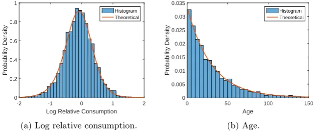
Figure 3.1 shows the histograms of log relative consumption and age at

t = 1 for one simulation. Since the burn in period is 10/δ = 300, this is ac-tually the 301st observation from the simulated data. The solid lines show the theoretical densities. For log consumption, the density is the convolution of the normal N(−τ2_{/2, τ}2_{) with τ}2 _=σ2

0+σǫ2 (coming from idiosyncratic shock

at birth and log measurement error) and the logarithm of double Pareto with exponentsα1, α2(which is known asLaplace (Kotz et al., 2001)). The resulting

distribution is known as normal-Laplace, which is the logarithm of the double Pareto-lognormal and has a known closed-form density function (Reed and Jor-gensen, 2004). Since the birth/death probability is constant, the theoretical age distribution is geometric (exponential). According to Figure 3.1, the theoretical densities closely track the histograms, so the continuous-time approximation is very good.

Although the histogram of log consumption is bell-shaped and may appear to be normal, actually it is far from normal. First, it is asymmetric because the two power law exponents α1 = 4.53 andα2 = 3.53 are distinct (the lower tail

is fatter). Second, since consumption has power law tails, log consumption has exponential tails, which are fatter than those of the normal distribution. To see

13

-2 -1 0 1 2 Log Relative Consumption 0

0.2 0.4 0.6 0.8 1

Probability Density

Histogram Theoretical

(a) Log relative consumption.

0 50 100 150

Age 0

0.005 0.01 0.015 0.02 0.025 0.03 0.035

Probability Density

Histogram Theoretical

(b) Age.

Figure 3.1: Histograms of cross-sectional distributions att= 1.

this graphically, Figure 3.2 shows the QQ (quantile-quantile) plot of log relative consumption against the normal distribution (fitted by maximum likelihood) and the normal-Laplace distribution (with the theoretical parameters). If the statistical model fits well to data, the QQ plot should show a 45 degree line. According to the result with the normal distribution (Figure 3.2a), the points deviate from the 45 degree line in the tails, which suggests that log consumption has much fatter tails than normal. On the other hand, the result with the normal-Laplace distribution (Figure 3.2b) shows a straight line, so the simulated data is close to the theoretical distribution.

-2 -1 0 1 2

Quantiles of fitted normal -2

-1 0 1 2

Quantiles of data

(a) Normal.

-2 -1 0 1 2

Quantiles of theoretical normal-Laplace -2

-1 0 1 2

Quantiles of data

(b) Normal-Laplace.

Figure 3.2: QQ plot of log relative consumption att= 1.

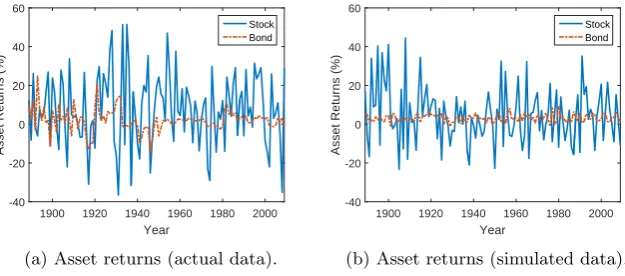
Figures 3.3 shows the actual (1889–2009) and simulated (first 121 years) asset returns, which show similar patterns.

4

Monte Carlo study

1900 1920 1940 1960 1980 2000 Year

-40 -20 0 20 40 60

Asset Returns (%)

Stock Bond

(a) Asset returns (actual data).

1900 1920 1940 1960 1980 2000 Year

-40 -20 0 20 40 60

Asset Returns (%)

Stock Bond

(b) Asset returns (simulated data).

Figure 3.3: Asset returns from actual and simulated data.

cross-sectional moment of consumption does not exist at the true γ, we expect that the MU SDF will perform poorly because the large sample limit of the GMM criterion is random.

We consider the possibility of both a Type I error (incorrect rejection of a true null) and a Type II error (incorrect non-rejection of a false null). Two sorts of Type I errors are possible in our setting. First, the nonexistence of cross-sectional moments could prevent the true model from explaining the equity premium. Indeed, according toχ2_{tests of overidentifying restrictions, standard}

GMM over-rejects the true model. Second, inconsistency could lead us to find excessively high γ estimates and reject lower but correct values. This is what we find. Type II errors may arise precisely because the power law behavior lets us zero the pricing error at spuriously highγestimates. Often, we fail to reject the model even when the asset returns are completely random.

4.1

GMM estimation

4.1.1 Standard GMM

The standard GMM proceeds as follows. Let

gT(γ) =

1

T

T

X

t=1

b

mMUt (γ)(Rst−R f

t−1)⊗zt−1

be the sample average of the pricing errors for the equity premium, whereT is the number of time periods, mbMU

t (γ) is the MU stochastic discount factor in

(2.4), Rs

t is the model-generated asset returns, R f

t−1 is the risk-free rate, and

zt−1is the vector of instruments. As described in the introduction, we consider

three different specifications forRs

t andzt−1. For the “exactly identified” model,

the only asset is the dividend claim (Rs

t =Rdt), and there are no instruments.

Instruments are not necessary for estimation but are necessary for tests of overi-dentifying restrictions if there is only one asset. Therefore, we also consider the “conditional” model. In this case, the dividend claim is still the only asset, but we use two instruments, the constant 1 and the normalized price-dividend ratio defined to bePt−1/Dt−1 divided by its sample mean. As the exactly identified

has two assets, a claim on dividends and consumption (Rs

t= (Rtc, Rdt)), but no

instruments. See Online Appendix for a comparison of all three specifications. LettingW be the weighting matrix (we choose the identity matrix for the first stage estimation), the GMM estimator of the relative risk aversion coeffi-cientγ and the mean squared pricing error are defined by

b

γ= arg min

γ T gT(γ)

′_{W g}

T(γ),

e=

q

kgT(bγ)k2/K=kgT(bγ)k/

√

K,

whereKis the number of equations in GMM.14_SincembMU

t (γ) andzt−1are

num-bers close to 1, the mean squared pricing errorehas the same order of magnitude as the equity premium. This definition makes the comparison across different models intuitive, unlike the minimized GMM criterion which tends to be larger for overidentified models. Note, however, that since the first stage weighting matrix is the identity matrix, the mean squared error is just a monotonic trans-formation of the minimized GMM criterion. The calculation of standard errors and test statistics are explained in Online Appendix.15

In addition to standard GMM using the identity matrix as the weighting matrix, we also consider the generalized empirical likelihood (GEL) approach of Kitamura and Stutzer (1997) since GEL estimators are known to have smaller bias (Newey and Smith, 2004). Although there are many variants of GEL (see Kitamura (2007) for a review), the one that uses the Kullback-Leibler informa-tion as in Kitamura and Stutzer (1997) is particularly convenient because the dual optimization problem is unconstrained and low dimensional.

4.1.2 Age cohort GMM

As discussed in Section 2.2, the standard GMM is inconsistent when the con-sumption distribution has fat tails. To mitigate this issue, Toda and Walsh (2015) propose “age cohort GMM”. Since the Euler equation aggregation in Section 2.1 that gave us the SDFs also works within a particular age cohort, and since the cross-sectional distribution of consumption is lognormal within age cohorts according to the model in Section 3, we can estimate an overiden-tified model by dividing agents into age groups. For example, divide the agents into H age groups according to the 100h/H percentile of the age distribution (h= 1, . . . , H), and call these groupsIt,1, . . . , It,H. We can form the MU SDF

for cohort hby

b

mMU t,h(γ) =

1

|It,h|

P

i∈It,hc

−γ it 1

|It−1,h|

P

i∈It−1,h

c−_i,tγ₋₁,

where|It,h|is the number of households in groupIt,h. One caveat is that since

an agent with ageaat timet−1 will have agea+ 1 at timet(if alive) and since

14

In implementing the minimization overγ, to avoid local minima that are not the global minimum, we first perform a grid search overγ= 0,1,2, . . . ,20 and then use the minimizer as the initial value for thefminconcommand in Matlab (with constraintγ≥0). We supply the analytical gradients to speed up the minimization.

15

each Euler equation is agent specific, the age cutoffs for the numerator must be +1 of those of the denominator.

LetmbMU_t (γ) = (mbMU

t,1 (γ), . . . ,mbMUt,H(γ))′ be the vector of SDFs and

GT(γ) =

1

T

T

X

t=1

b

mMU_t (γ)⊗(Rst−R f

t−1)⊗zt−1

be the vector of pricing errors. Letting W be the weighting matrix, the first stage GMM estimator ofγ and the mean squared pricing error are

b

γ= arg min

γ T GT(γ)

′_{W G}

T(γ),

e=

q

kGT(bγ)k2/(KH) =kGT(bγ)k/

√

KH,

where K is the number of equations in each cohort and H is the number of cohorts. Below, we choose H = 5 (five age cohorts) and set the weighting matrix to the identity matrix.

4.1.3 Representative-agent GMM

Finally, as a robustness check, we also estimateγfrom the representative-agent model (RA), which turns out to be valid for this particular example.16 _{To see}

this, dividing both sides of the first-order condition (A.1) byc−itγPtd, we obtain

1 = ˜βEt

(ci,t+1/cit)−γRdt+1

,

whereRd

t+1= (Pt+1d +Dt+1)/Ptdis the dividend claim return. Since by (3.2) log

individual consumption growth is equal to log aggregate consumption growth plus the idiosyncratic shock, it follows that

1 = ˜βe12γ(γ+1)σ 2

Et

(Ct+1/Ct)−γRdt+1

.

The same equation holds for the consumption claim and the risk-free rate. Tak-ing the difference and dividTak-ing by ˜βe12γ(γ+1)σ

2

, we obtain the moment condition

Et

h

(Ct+1/Ct)−γ(Rt+1d −Rtf)

i

= 0.

Therefore up to a multiplicative constant, mRA

t+1(γ) = (Ct+1/Ct)−γ is also a

valid stochastic discount factor. The GMM estimation of this representative-agent model is completely analogous.

16

4.2

Type I error

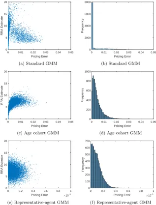
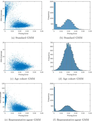
To study the possibility of a Type I error, we use the model-simulated consump-tion, stock, and bond return data and estimate each model by GMM. From top to bottom, Figure 4.1 shows the conditional model results for standard GMM, age cohort GMM, and representative-agent GMM with sample sizeT = 500.17

The left panels show the scatter plot of simulated γ estimates and normalized mean squared pricing errors for 10,000 simulations. The right panels show the histogram of the pricing errors.

According to Figure 4.1a, across simulations there is an inverse relationship between the MUγestimate and the pricing error. When the MU model almost exactly zeroes the pricing error, theγestimate is often well above both the start of the moment nonexistence range,>4, and the true coefficient, 7.

However, splitting households into age groups and performing the age cohort GMM, we no longer see this pattern: the largeγestimates corresponding to the zero pricing errors in Figure 4.1a have disappeared in the age cohort GMM of Figure 4.1c. Indeed, according to the histogram of the pricing errors in Figures 4.1b and 4.1d, there is much less mass around zero with the age cohort method. And, according to the scatter plots, this mass is the result of upwardly biased estimates in the nonexistence range. As we see in the scatter plot in Figure 4.1e, the RA γ estimates seem to be unbiased compared to the age cohort GMM, although they have larger standard errors because the representative-agent model exploits fewer moment restrictions. Also, the pricing errors are almost negligible. (Note that the scale of the horizontal axis is 10−3_.)

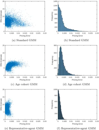
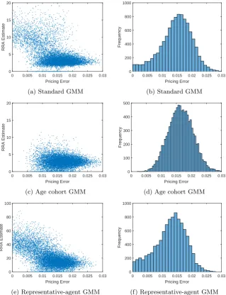
Figure 4.2 is the same as 4.1 but with the unconditional specification, which has consumption and dividend claims but no instruments. While the patterns are similar with respect to RA and age cohort GMM, standard GMM is some-what improved: there is less pricing error mass at zero corresponding to up-wardly biased estimates. As we discuss in Section 4.4, the improvements from the age cohort and unconditional specifications suggest overidentification miti-gates the adverse impact of fat tails on standard GMM.

Table 4.1 show the bias (the average ofbγ−γacross simulations), mean stan-dard error truncated at 100 (to avoid excessively large numbers that appear in the standard and representative-agent GMM but not age cohort), mean abso-lute error (MAE, the average of|bγ−γ|), and root mean squared error (RMSE, square root of the average of|bγ−γ|2) of each model/specification combination. For both the conditional and unconditional model, the age cohort GMM is the most biased but has the best finite sample properties in terms of standard er-ror, mean absolute erer-ror, and root mean squared error. Using the unconditional model improves standard errors, MAEs, and RMSEs but worsens the bias for standard GMM (while lessening it with the other models).

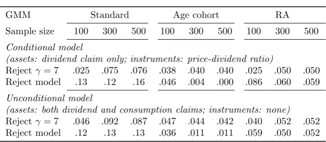
Table 4.2 shows the Type I error probabilities, corresponding to a signifi-cance level of .05. For T > 100, in the standard GMM columns we see the manifestation of the high bγ, low pricing error combinations in Figures 4.1a and 4.2a. With both the conditional and unconditional specifications, standard GMM over-rejects the true null (γ = 7), with sizes ranging from .075 to .092. In contrast, for T >100 age cohort and RA sizes range from .040 to .052. χ2

tests of overidentifying restrictions show that standard GMM also over-rejects

17

0 0.01 0.02 0.03 0.04 0.05 Pricing Error

0 5 10 15 20

RRA Estimate

(a) Standard GMM

0 0.01 0.02 0.03 0.04 0.05 Pricing Error

0 2000 4000 6000 8000

Frequency

(b) Standard GMM

0 0.01 0.02 0.03 0.04 0.05 Pricing Error

0 5 10 15 20

RRA Estimate

(c) Age cohort GMM

0 0.01 0.02 0.03 0.04 0.05 Pricing Error

0 200 400 600 800 1000

Frequency

(d) Age cohort GMM

0 0.2 0.4 0.6 0.8 1

Pricing Error ×10-3

0 5 10 15 20

RRA Estimate

(e) Representative-agent GMM

0 0.2 0.4 0.6 0.8 1

Pricing Error ×10-3

0 100 200 300 400 500 600 700

Frequency

(f) Representative-agent GMM

Figure 4.1: GMM estimation of conditional model (assets: dividend claim; in-struments: P/D ratio). Left: scatter plot of γ estimates and pricing errors. Right: histogram of pricing errors. T = 500.

the true model, while age cohort under-rejects and RA has the correct size. Overall, this exercise suggests that the nonexistent moments lead to low, over-fit pricing errors with highγ estimates in many instances and excessively high pricing errors in others. On net, this leads standard GMM to over-reject both the true parameter and model.

0 0.005 0.01 0.015 0.02 0.025 0.03 Pricing Error

0 5 10 15 20

RRA Estimate

(a) Standard GMM

0 0.005 0.01 0.015 0.02 0.025 0.03 Pricing Error

0 200 400 600 800 1000 1200 1400

Frequency

(b) Standard GMM

0 0.005 0.01 0.015 0.02 0.025 0.03 Pricing Error

0 5 10 15 20

RRA Estimate

(c) Age cohort GMM

0 0.005 0.01 0.015 0.02 0.025 0.03 Pricing Error

0 200 400 600 800

Frequency

(d) Age cohort GMM

0 0.005 0.01 0.015 0.02 0.025 0.03 Pricing Error

0 5 10 15 20

RRA Estimate

(e) Representative-agent GMM

0 0.005 0.01 0.015 0.02 0.025 0.03 Pricing Error

0 200 400 600 800 1000

Frequency

(f) Representative-agent GMM

Figure 4.2: GMM estimation of unconditional model (assets: dividend and consumption claims; instruments: none). Left: scatter plot of γ estimates and pricing errors. Right: histogram of pricing errors. T = 500.

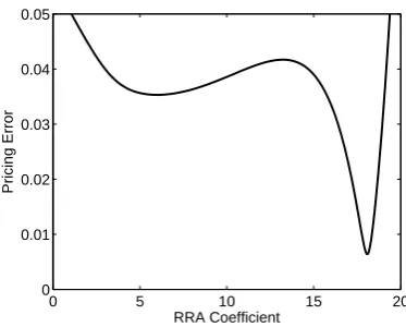
inflection points, yielding one trough near the true γ and one or more in the moment nonexistence range. It seems nonexistent moments may introduce spu-rious troughs, and in some instances, a spuspu-rious one is closest to zero. Figure 4.3 illustrates this scenario. In this figure, there is a trough atγ= 5.98, which is close to the true value (7) but not the global minimum. The other trough at

Table 4.1: Finite sample properties

GMM Standard Age cohort RA Sample size 100 300 500 100 300 500 100 300 500 Conditional model

(assets: dividend claim only; instruments: price-dividend ratio)

Bias -1.39 -.69 -.23 -2.02 -1.05 -.67 .48 .048 .043 SE100 10.9 7.44 6.36 3.09 2.17 1.82 4.88 2.72 2.10 MAE 3.23 2.32 2.04 2.41 1.61 1.33 3.85 2.18 1.67 RMSE 3.96 2.94 2.69 3.13 2.11 1.72 4.95 2.75 2.11 Unconditional model

(assets: both dividend and consumption claims; instruments: none)

Bias -1.79 -.92 -.56 -1.84 -.95 -.61 .37 .066 .064 SE100 6.42 4.13 3.28 2.64 1.87 1.56 4.06 2.33 1.80 MAE 2.73 1.91 1.57 2.15 1.42 1.16 3.28 1.88 1.45 RMSE 3.29 2.37 1.98 2.81 1.85 1.49 4.15 2.38 1.82

Note: SE100 denotes the mean of standard errors ofbγtruncated at 100. MAE is the mean absolute error (average of|bγ−γ|across simulations). RMSE is the root mean squared error (square root of the average of|bγ−γ|2

across simulations).

Table 4.2: Type I error probabilities

GMM Standard Age cohort RA Sample size 100 300 500 100 300 500 100 300 500 Conditional model

(assets: dividend claim only; instruments: price-dividend ratio)

Rejectγ= 7 .025 .075 .076 .038 .040 .040 .025 .050 .050 Reject model .13 .12 .16 .046 .004 .000 .086 .060 .059 Unconditional model

(assets: both dividend and consumption claims; instruments: none) Rejectγ= 7 .046 .092 .087 .047 .044 .042 .040 .052 .052 Reject model .12 .13 .13 .036 .011 .011 .059 .050 .052

Note:γ= 7: t-test. Model: χ2

test of overidentifying restrictions. Significance level: .05.

4.3

Type II error

To study the possibility of a Type II error, we use the model-simulated con-sumption data in conjunction withfalse asset returns data. More precisely, we generate a random permutation of the time index, and we use the model asset returns for this time index coupled with the consumption data of the calendar time. Because the equity premium is the same (2.11%) as with the true process and because the stochastic discount factor is always positive, the independence of the SDF and the excess stock returns (which holds by construction) implies that in large samples the moment conditiondoes not hold.

0 5 10 15 20 0

0.01 0.02 0.03 0.04 0.05

RRA Coefficient

Pricing Error

Figure 4.3: Normalized mean squared pricing error from a simulation with two troughs. Model: standard GMM. Specification: conditional (assets: dividend claim; instruments: P/D ratio).

The left panels show the scatter plot of simulated γ estimates and normalized mean squared pricing errors for 10,000 simulations. The right panels show the histogram of the pricing errors.

Figure 4.4b shows the histogram of the pricing errors estimated by standard GMM. In 1877 out of 10,000 simulations, the pricing errors are within 10−3 _of

zero! With age cohort GMM (Figure 4.4d), in contrast, only 7 of 10,000 simu-lations yield pricing errors within 10−3 _{of zero. Also, the age cohort histogram}

is centered on about 2%, exactly as one would expect since the true equity premium is 2.11% and the pricing errors are normalized. Oddly, however, the standard GMM pricing error histogram is bimodal, with one peak at 2% and the other at zero. Moreover, as we see in Figures 4.4a and 4.4c, the spurious mode at zero is driven by upwardly biased estimates in the nonexistence range. This behavior is odd but perhaps unsurprising given the findings of Toda and Walsh (2015): the bootstrapped scatter plots and histograms of that analysis displayprecisely the same pattern!

Figure 4.5 is the same as 4.4 but with the unconditional specifications. As with Type I errors, switching from the conditional to unconditional model, which has two assets but no instruments, mitigates somewhat the spurious mass at zero for standard GMM (and for the RA model as well). However, Figures 4.5b and 4.5f still exhibit excess mass at zero, relative to age cohort, corresponding to highγ estimates.

Thus the standard GMM seems to lead to Type II errors (incorrect non-rejection of a false model) due to excessively low pricing errors. We can see formally the low power of standard GMM by comparing the histograms of the pricing errors of the true and false models. For example, under the null (con-sumption and return data generated from the true model), for standard GMM with the conditional specification (T = 500) the 95 percentile of the pricing error is .0139. Since the number of pricing errors larger than .0139 with the false model is 5756 out of 10,000 simulations, the rejection rate (power) is only 57.6%. On the other hand, for age cohort GMM, it is 91.6%.

0 0.01 0.02 0.03 0.04 0.05 Pricing Error

0 5 10 15 20

RRA Estimate

(a) Standard GMM

0 0.01 0.02 0.03 0.04 0.05 Pricing Error

0 500 1000 1500 2000 2500

Frequency

(b) Standard GMM

0 0.01 0.02 0.03 0.04 0.05 Pricing Error

0 5 10 15 20

RRA Estimate

(c) Age cohort GMM

0 0.01 0.02 0.03 0.04 0.05 Pricing Error

0 100 200 300 400 500 600 700

Frequency

(d) Age cohort GMM

0 0.01 0.02 0.03 0.04 0.05 Pricing Error

0 20 40 60 80 100 120

RRA Estimate

(e) Representative-agent GMM

0 0.01 0.02 0.03 0.04 0.05 Pricing Error

0 500 1000 1500 2000 2500

Frequency

(f) Representative-agent GMM

Figure 4.4: GMM estimation of conditional model (assets: dividend claim; in-struments: P/D ratio) with false stock returns. Left: scatter plot ofγestimates and pricing errors. Right: histogram of pricing errors. T = 500.

shows the result for the exact test just described using pricing errors. “Asymp-totic χ2 _{test” uses the χ}2 _{statistic from the first stage GMM and the critical}

value from the asymptotic distribution. “Exactχ2_{test” uses the sameχ}2

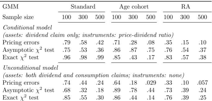
statis-tic but obtains the cristatis-tical value as the simulated 95 percentile under the null. The standard GMM is a disaster. Even with T = 500 and using the uncondi-tional specification, the Type II error probability is 18 to 30 percent, depending on the test. With the conditional model, the range is 36 to 99 percent! The representative-agent GMM is similar when using theχ2_{statistic, although the}

0 0.005 0.01 0.015 0.02 0.025 0.03 Pricing Error

0 5 10 15 20

RRA Estimate

(a) Standard GMM

0 0.005 0.01 0.015 0.02 0.025 0.03 Pricing Error

0 200 400 600 800 1000

Frequency

(b) Standard GMM

0 0.005 0.01 0.015 0.02 0.025 0.03 Pricing Error

0 5 10 15 20

RRA Estimate

(c) Age cohort GMM

0 0.005 0.01 0.015 0.02 0.025 0.03 Pricing Error

0 100 200 300 400 500

Frequency

(d) Age cohort GMM

0 0.005 0.01 0.015 0.02 0.025 0.03 Pricing Error

0 20 40 60 80 100

RRA Estimate

(e) Representative-agent GMM

0 0.005 0.01 0.015 0.02 0.025 0.03 Pricing Error

0 200 400 600 800 1000

Frequency

(f) Representative-agent GMM

Figure 4.5: GMM estimation of unconditional model (assets: dividend and consumption claims; instruments: none) with false stock returns. Left: scatter plot ofγ estimates and pricing errors. Right: histogram of pricing errors. T = 500.

small under the correct null. In contrast, the age cohort GMM has much higher power with respect to the pricing error and exact χ2 _{test: the Type II error}

probability is around 3 to 17 percent, depending on the specification and test. Age cohort GMM, however, performs poorly with respect to the asymptoticχ2

test.

over-Table 4.3: Type II error probabilities

GMM Standard Age cohort RA Sample size 100 300 500 100 300 500 100 300 500 Conditional model

(assets: dividend claim only; instruments: price-dividend ratio)

Pricing errors .79 .58 .42 .71 .28 .08 .35 .15 .10 Asymptoticχ2 _{test .75 .53 .36 .86 .87 .75 .76 .54 .37}

Exactχ2_{test .96 .98 .99 .85 .43 .17 .83 .57 .38}

Unconditional model

(assets: both dividend and consumption claims; instruments: none)

Pricing errors .74 .44 .24 .64 .18 .029 .33 .10 .057 Asymptoticχ2 _{test .68 .32 .18 .89 .78 .44 .73 .39 .24}

Exactχ2_{test .85 .55 .30 .86 .44 .14 .76 .39 .25}

Note: The table shows, with respect to different tests, the probability of failing to reject that the model explains false, randomly generated returns. See text for explanations of the various tests. Significance level: .05.

fitting of models. This conjecture seems to hold for the representative-agent model as well. In this case, aggregate consumption growth is lognormal, so the tails are thin. However, by raising a lognormal variable to a high power, we can get tails that are quite fat. As in the case with standard GMM, the histogram of representative-agent GMM in Figure 4.4f shows a bimodal pattern. In 2172 out of 10,000 simulations, the pricing errors are within 10−3 of zero, and the spurious mode at zero is driven by upwardly biased estimates ofγaround 20 to 80 according to the scatter plot in Figure 4.4e.

4.4

Source of bimodal pricing errors

What is the source of bimodality in the pricing error, with a spurious peak at zero?18 _{We can provide an intuitive explanation as follows. Consider the}

GMM estimation of the representative-agent model with no instruments (single equation). Then the GMM estimator is the solution of

1

T

T

X

t=1

(Ct/Ct−1)−γ(Rts−R f

t−1) = 0. (4.1)

For notational simplicity, let Gt = Ct/Ct−1 be the aggregate consumption

growth and Xt=Rst−Rft−1 be the excess stock market return. Furthermore,

relabel time so that G1≤G2≤ · · · ≤GT. Then (4.1) becomes

1

T

T

X

t=1

G−tγXt= 0. (4.2)

18

Since{Gt}Tt=1 is sorted in ascending order andγ >0, we haveG

−γ 1 ≫G

−γ 2 ≫

· · · ≫G−_Tγ. Hence the first two terms dominate the others, and (4.2) becomes

G−1γX1+G−2γX2= 0 (4.3)

approximately. But provided thatX1, X2 have opposite signs and|X2|>|X1|,

(4.3) has a solution

γ=log(−X2/X1) log(G2/G1)

>0. (4.4) SinceGt’s are sorted in ascending order,G1 andG2 are relatively close to each

other, so log(G2/G1) is a small positive number. Therefore the γ estimate in

(4.4) will typically be a large number. Note that this argument holds regardless of whether the model is true or false. If asset returns are completely random, we would expect that we can make the pricing error close to zero with probability Pr(−X2/X1>1), which will be the probability of Type II errors.

The same argument holds for the standard GMM estimation with MU SDF. Recall that the MU SDF is defined by

b

mMU t (γ) =

1 I

PI i=1c

−γ it 1

I

PI i=1c

−γ i,t−1

.

When cross-sectional consumption has fat tails, the terms corresponding to the minimum consumption at each period dominate, and we have

b

mMUt (γ)≈ 1

I(minicit)

−γ 1

I(minici,t−1)−γ

=

minicit

minici,t−1

−γ

.

Thus the same argument holds by replacingCt/Ct−1in (4.1) by minicit/minici,t−1.

In particular, the MUγ estimates from standard GMM will be biased upwards as in Figures 4.1a and 4.4a because the γ given by (4.4) tends to be large. In Section 2.2 we showed formally that GMM minimizes a random functionZ(γ)2_,

and we now have an intuitive explanation for this phenomenon: the GMM es-timate depends on random outlier draws, even whenT is large.

Now we can see what the age cohort GMM achieves. For a false model, the pricing error is spuriously set to zero at the γ given by (4.4). Note that this γ depends on the value of G2/G1, the fraction between the two smallest

observations. With the MU SDF, Gt corresponds to minicit/minici,t−1. By

dividing agents into age cohorts, the value of minicit/minici,t−1for each cohort

will in general be distinct. Therefore except for by chance, it would not be possible to set the pricing errors simultaneously zero across age cohorts. Only if the model is true can we set the pricing errors simultaneously zero at the true

γ. This gives age cohort GMM statistical power higher than that of standard GMM. A similar argument holds for the unconditional specification with two assets since the signs of Rct−R

f

t−1 andRdt −R f

t−1 will often not be the same.

Standard GMM, in contrast, may zero the pricing error at the arbitraryγfrom (4.4) whether or not returns are generated from the true model.

5

Conclusion

prices and a fat tailed consumption distribution from a tractable incomplete-market dynamic general equilibrium model and show in a Monte Carlo study that there are potential pitfalls to this practice of averaging: in the presence of fat tails in the cross-section, the resulting GMM criterion may contain sample analogs of nonexistent moments, which diverge in large samples. We establish that fat tails in consumption create over-rejection of true models/parameters and Type II errors (non-rejection of incorrect models) in the standard aggre-gated Euler equation GMM estimation of the relative risk aversion coefficient. The “age cohort” estimation method suggested in Toda and Walsh (2015) ap-pears to mitigate these problems. Our broad message is that standard inference methods may be invalid in settings prone to power laws.

When should we worry about fat tails, and what should we do to avoid spu-rious estimation? Our Monte Carlo exercise sheds some light on these issues. First, even the representative-agent model (which does not have fat tails) is prone to spurious estimation by raising a positive random variable (here con-sumption growth) to a high power, which makes the tails fatter. So one should be careful when estimating a model that involves a power function. Second, spurious estimation seems to result from minimizing the sample GMM criterion by canceling the two outliers with opposite signs. Since the location of this spurious trough is random, estimating an overidentified model will likely miti-gate the problem. Finally, when in doubt we can always conduct a bootstrap exercise, for example the stationary bootstrap of Politis and Romano (1994). According to the findings of Toda and Walsh (2015), a bimodal histogram of bootstrapped GMM criterions suggests spurious estimation.

A

Asset prices

Since agents have identical homothetic preferences and all shocks are multiplica-tive (addimultiplica-tive in logs), it is known that even if there are arbitrarily many assets, as long as the payoffs of the assets do not depend on idiosyncratic shocks, there will be no trade in assets in equilibrium, that is, the equilibrium is autarky (Constantinides and Duffie, 1996; Krueger and Lustig, 2010; Toda, 2014). Thus individual consumptioncitequals individual endowment yit. By the first-order

condition for the stock, we have

cit−γPtd= ˜βEt[ci,t+1−γ (Pt+1d +Dt+1)], (A.1)

where Pd

t is the price of the dividend claim and ˜β =β(1−δ) is the effective

discount factor. Dividing both sides byc−_itγDt and defining the price-dividend

ratio in statextbyVd(xt) :=Ptd/Dt, we obtain

Vd(xt) = ˜βEt[(ci,t+1/cit)−γ(Dt+1/Dt)(Vd(xt+1) + 1)]

= ˜βEt[exp (−γlog(Ct+1/Ct)−γεi,t+1+ log(Dt+1/Dt)) (Vd(xt+1) + 1)].

Lettingvd= (−γ,1)′ and using the fact thatεitis i.i.d., we obtain

Vd(xt) = ˜βEt[exp(−γεi,t+1)] Et[exp(v′dxt+1)(Vd(xt+1) + 1)]

= ˜βe12γ(γ+1)σ 2

where we have used

E[exp(−γε)] =

Z ∞

−∞

e−γx√1

2πσe

−(x+σ2/2)2

2σ2 dx

=

Z ∞

−∞

e12γ(γ+1)σ

2 1

√

2πσe

−(x+(γ+1_2σ/22)σ2 )2_{dx= e}12γ(γ+1)σ 2

if ε ∼ N(−σ2_{/2, σ}2_{). When {x}

t} follows a VAR(1) process (3.1), Burnside

(1998) iterates (A.2) and obtains a closed-form solution as follows. Let ˜

Σ = (I−A)−1Σ(I−A′)−1,

Σn= n

X

k=1

AkΣ(˜ A′)k,

Bn= n

X

k=1

Ak =A(I−An)(I−A)−1,

Ωn=nΣ˜ −BnΣ˜−Σ˜Bn′ + Σn.

Then we have

Vd(x) =

∞

X

n=1

˜

βnexp

1

2γ(γ+ 1)σ

2_+v′

dg

n+vd′Bn(x−g) +

1 2v

′

dΩnvd

.

(A.3) It is easy to show that this series converges if and only if

˜

βexp

1

2γ(γ+ 1)σ

2_+v′

dg+

1 2v

′

dΣ˜vd

<1. (A.4) Sincevd= (−γ,1)′, inside of the exponential is a quadratic function in each ofσ

andγ. Therefore in order for an equilibrium to exist, the idiosyncratic volatility

σor risk aversionγ cannot be too high.

We can compute the asset returns as follows. Letxt= (x1t, x2t)′. Then the

dividend growth is Dt+1/Dt= ex2,t+1, and the stock return is

Rd t+1=

Pd

t+1+Dt+1

Pd t

= (P

d

t+1/Dt+1+ 1)(Dt+1/Dt)

Pd t/Dt

=Vd(xt+1) + 1

Vd(xt)

ex2,t+1_.

(A.5) We can compute the return to the consumption claim similarly by computing

Vc(xt) as in (A.2) withvc = (1−γ,0)′ instead ofvd and using (A.5) to define

Rc

t+1 withVc, x1,t+1 instead ofVd, x2,t+1. The calculation of the risk-free rate

Rft is similar. Letting vf = (−γ,0)′, by the Euler equation we have

1

Rft

= ˜βEt[(ci,t+1/cit)−γ] = ˜βEt[exp(−γlog(Ct+1/Ct)−γεi,t+1)]

= ˜βexp

1

2γ(γ+ 1)σ

2_+v′

f(g+A(xt−g)) +

1 2v

′

fΣvf

. (A.6)

References

Joseph G. Altonji and Lewis M. Segal. Small-sample bias in GMM estimation of covariance structures. Journal of Business and Economic Statistics, 14(3): 353–366, July 1996. doi:10.1080/07350015.1996.10524661.

Donald W. K. Andrews and Xu Cheng. Estimation and inference with weak, semi-strong and strong identification. Econometrica, 80(5):2153–2211, September 2012. doi:10.3982/ECTA9456.

Pierluigi Balduzzi and Tong Yao. Testing heterogeneous-agent models: An alternative aggregation approach. Journal of Monetary Economics, 54(2): 369–412, March 2007. doi:10.1016/j.jmoneco.2005.08.021.

Parantap Basu, Andrei Semenov, and Kenji Wada. Uninsurable risk and fi-nancial market puzzles. Journal of International Money and Finance, 30(6): 1055–1089, October 2011. doi:10.1016/j.jimonfin.2011.05.012.

Erich Battistin, Richard Blundell, and Arthur Lewbel. Why is consumption more log normal than income? Gibrat’s law revisited. Journal of Political Economy, 117(6):1140–1154, December 2009. doi:10.1086/648995.

Marie-Claude Beaulieu, Jean-Marie Dufour, and Lynda Khalaf. Asset-pricing anomalies and spanning: Multivariate and multifactor tests with heavy-tailed distributions. Journal of Empirical Finance, 17(4):763–782, September 2010. doi:10.1016/j.jempfin.2010.03.001.

Jess Benhabib, Alberto Bisin, and Shenghao Zhu. The distribution of wealth and fiscal policy in economies with finitely lived agents. Econometrica, 79(1): 123–157, January 2011. doi:10.3982/ECTA8416.

Jess Benhabib, Alberto Bisin, and Shenghao Zhu. The distribution of wealth in the Blanchard-Yaari model. Macroeconomic Dynamics, 20:466–481, March 2016. doi:10.1017/S1365100514000066.

Istv´an Berkes and Lajos Horv´ath. The rate of consistency of the quasi-maximum likelihood estimator. Statistics and Probability Letters, 61(2):133–143, Jan-uary 2003. doi:10.1016/S0167-7152(02)00342-5.

Olivier J. Blanchard. Debt, deficits, and finite horizons. Journal of Political Economy, 93(2):223–247, April 1985.

Alon Brav, George M. Constantinides, and Christopher C. Geczy. Asset pricing with heterogeneous consumers and limited participation: Empiri-cal evidence. Journal of Political Economy, 110(4):793–824, August 2002. doi:10.1086/340776.

Douglas T. Breeden. An intertemporal asset pricing model with stochastic consumption and investment opportunities. Journal of Financial Economics, 7(3):265–296, September 1979. doi:10.1016/0304-405X(79)90016-3.

Leo Breiman. Probability. Addison Wesley, Reading, MA, 1968.