Munich Personal RePEc Archive
Zipf’s Law: A Microfoundation
Toda, Alexis Akira
University of California, San Diego
30 September 2016
Zipf’s Law: A Microfoundation
Alexis Akira Toda
∗This version: April 30, 2017
Abstract
Existing explanations of Zipf’s law (Pareto exponent approximately equal to 1) in size distributions require strong assumptions on growth rates or the minimum size. I show that Zipf’s law naturally arises in general equilibrium when individual units solve a homogeneous problem (e.g., homothetic preferences, constant-returns-to-scale technology), the
units enter/exit the economy at a small constant rate, and at least one production factor is in limited supply. My model explains why Zipf’s law is empirically observed in the size distributions of cities and firms, which consist of people, but not in other quantities such as wealth, income, or consumption, which all have Pareto exponents well above 1.
Keywords: Gibrat’s law, homogeneous problem, power law
JEL codes: D30, D52, D58, L11, R12
1
Introduction
Zipf’s law is an empirical regularity that holds in the size distributions of cities and firms, stating that the frequency of observing a unit larger than the cutoff xis approximately inversely proportional tox:
P(X > x)∼x−ζ,
where the Pareto (power law) exponentζ is slightly above 1. This relationship holds regardless of the choice of countries or time periods.1 To get a sense of
∗
Department of Economics, University of California San Diego. Email: [email protected]. I thank Marios Angeletos, Eli Berman, Alberto Bisin, Harold Cole, Darrell Duffie, Xavier Gabaix, Simon Gilchrist, Rishabh Kirpalani, Narayana Kocherlakota, Makoto Nirei, Jim Rauch, Venky Venkateswaran, and seminar participants at Chinese University of Hong Kong, City University of Hong Kong, Fudan, Keio, Kobe University Research Institute for Economics and Business Administration, NYU Stern, Osaka, UCSD, and Cowles Conference on General Equilibrium and its Applications for comments and feedback. Miles Berg and Xuan Fang have provided excellent research assistance.
1Although Zipf’s law is named after Zipf (1949), its discovery dates back at least to
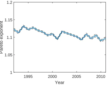
how the empirical size distribution looks like, Figure 1 shows a log-log plot of employment cutoffs and the number of firms larger than the cutoffs (essentially the ranks) using the 2011 U.S. Census Small Business Administration (SBA) data. Consistent with a power law, the figure shows a straight-line pattern up to small firms with as few as 10 employees. The Pareto exponent estimated by maximum likelihood isζb= 1.0967 with a standard error of 0.0020. We obtain similar patterns for all years from 1992 to 2011 for which data is available. Figure 2 shows the estimated Pareto exponent over the period 1992–2011, which is slightly above 1 in all years. As Krugman (1996) puts it, “there must be a compelling explanation of the astonishing empirical regularity.”
Employment cutoff
100 101 102 103 104
Number of larger firms
103 104 105 106
107 2011
[image:3.595.197.383.260.413.2]Data dPlN lognormal
Figure 1: Log-log plot of firm size distribution.
Note: The figure plots employment cutoffs and the number of firms larger than the cutoffs (ranks). dPlN stands fordouble Pareto-lognormal, which is a distribution arising from the theoretical model in the paper. The straight-line pattern is consistent with a power law, with estimated exponentζb= 1.0967 and standard error 0.0020 using maximum likelihood with binned data (sample sizeN = 5,684,424; see Appendix D for details). Source: 2011 U.S. Census Small Business Administration data.
1995 2000 2005 2010
Year 1
1.05 1.1 1.15 1.2
Pareto exponent
Figure 2: Time series of estimated Pareto exponent.
[image:3.595.197.386.503.650.2]In addition to its empirical regularity, Zipf’s law is important because it may explain aggregate fluctuations from a micro level (Gabaix, 2011) and has distinct welfare implications of entry cost and trade barriers (di Giovanni and Levchenko, 2013). In a seminal paper, Gabaix (1999) has shown that Zipf’s law arises when individual units follow Gibrat (1931)’s law of proportional growth and there is some small minimum size (relative to the average size) that the units must meet. His work has generated a large subsequent literature on power laws in economics and finance as well as models that attempt to explain Zipf’s law. But where does this condition, which is equivalent to the condition that the expected growth rate of existing units is small in absolute value relative to the variance, come from? Given that Zipf’s law is empirically so robust, an explanation of Zipf’s law should not depend on a fine-tuning of particular parameters. Instead, there must be a mechanism that delivers the small growth condition endogenously. This paper proposes a new mechanism that endogenously delivers the small growth condition, and hence provides a microfoundation for Zipf’s law.
My theory is surprisingly simple, and essentially relies on the following three elements: (i) Gibrat’s law of proportional growth, (ii) individual units enter-ing/exiting the economy with small probability (“rare disasters”), and (iii) ex-istence of a production factor that is mobile but in limited supply. Conditions (i) and (ii) have already been known to be sufficient for generating Pareto tails (Reed, 2001), but Zipf’s law (Pareto exponent close to 1) holds only in the knife-edge case in which the expected growth rate of units is small in absolute value. My contribution is thus in showing that condition (iii)—the existence of a production factor in limited supply, or to be precise, one production factor is bounded above by an exogenous process—limits aggregate growth, which in equilibrium also limits individual growth and delivers Zipf’s law. The intuition is as follows. If individual units solve a homogeneous problem (e.g., homoth-etic preferences, constant-returns-to-scale technology), the size of these units obeys Gibrat’s law of proportional growth. But if one of the production fac-tors is in limited supply, the aggregate economy exhibits decreasing returns to scale. Since the economy converges to the steady state (zero aggregate growth), and by accounting the aggregate is the sum of individuals, it follows that the individual growth rate endogenously becomes small. My theory explains why Zipf’s law is empirically observed only for cities and firms, but not for other quantities such as wealth, income, or consumption, which all obey power laws but with exponents well above 1.2 Cities and firms consist of people, which can
be thought of as a production factor that is in limited supply (bounded by an exogenous process). On the other hand, there is no obvious exogenous process that bounds wealth, income, or consumption.
To illustrate these points in the simplest possible way, I first construct a stylized model of the population dynamics of cities (villages). In the model, there are a continuum of villages and households. The village authorities pro-duce a single good (“potato”) using a constant-returns-to-scale technology and hiring labor. Households migrate across villages freely without any cost. Vil-lages are hit by two types of idiosyncratic shocks—technological shocks and rare disasters (“famine”). When a famine occurs, the potatoes in the village are wiped out, but the village authority receives deliveries of potatoes from other
2Reed (2003) and Toda (2012) find that the Pareto exponent for income is around 2. Toda
villages because they have a mutual insurance. This simple model has all the ingredients sufficient for generating Zipf’s law: (i) with multiplicative techno-logical shocks and constant-returns-to-scale technology, we obtain Gibrat’s law for individual villages, (ii) famines are reset events and generate a stationary distribution with Pareto tails, and (iii) the inelastic labor supply endogenously forces the expected population growth rate in individual villages to be small in equilibrium, generating Zipf’s law.
The intuition for this simple model carries over to more general models. Con-sider a dynamic general equilibrium model which consists of several agent types, and suppose that we are interested in the size distribution of an economic vari-able of a particular type (e.g., firm size distribution measured by the number of employees). The main result of this paper, Theorem 3.5, shows that if agents of this type solve a homogeneous problem (e.g., homothetic preferences, constant-returns-to-scale technology, proportional constraints), the agents enter/exit the economy at a constant rate η >0, and at least one factor of production is in limited supply, then Zipf’s law holds in the stationary equilibrium as η → 0. This result holds in a wide variety of models, including those with elastic labor supply, balanced growth, random initial size, multiple types, and discrete time with non-Gaussian shocks.
Because the main theorem is an asymptotic result, the Pareto exponent need not be close to 1 for particular models or parameter configurations. To address the quantitative validity of my theory, I construct a model of entrepreneurship and firm size distribution. The economy is populated by entrepreneur-CEOs and household-workers. Each entrepreneur operates a firm using a constant-returns-to-scale technology and hiring labor, and makes consumption-saving-portfolio-hiring decisions optimally. Entrepreneurs are subject to idiosyncratic investment risk and bankruptcy. Workers supply labor inelastically but make consumption-saving decisions optimally. In this setting under mild conditions I prove that a unique stationary equilibrium exists and characterize the equilibrium in closed-form. I prove that the stationary firm size distribution obeys Zipf’s law when the bankruptcy rate is small. I calibrate the model to the U.S. economy and find that the Pareto exponent is close to 1, consistent with Zipf’s law.
Given the empirical robustness of Zipf’s law, an “explanation” should not depend on a particular calibration of parameters. Hence to show its robustness, I generate random parameter configurations drawn from a uniform distribution with a large support (changing each parameter up to 5-fold independently), and for each case I compute the equilibrium Pareto exponent. For this particular model I find that the 95 percentile of the Pareto exponent is 1.13, so Zipf’s law holds even for quite extreme (and unrealistic) parameter configurations, confirming its robustness.
1.1
Related literature
Pareto (1896) discovered that the size distribution of income obeys a power law. The idea of using random growth models3 to explain power law
distri-3In this paper I focus on the random growth model because (i) it is the earliest model
butions dates back to Yule (1925), Champernowne (1953), Simon (1955), and Kesten (1973), among others. Because random proportional growth (Gibrat’s law) alone does not lead to a stationary distribution (one would get a lognor-mal distribution, whose log variance increases linearly over time), one needs to introduce additional assumptions. Champernowne (1953) introduces a mean-reverting force and obtains the double Pareto distribution; Wold and Whittle (1957) consider random birth and death; Kesten (1973) considers both mul-tiplicative and additive shocks. For reviews of generative mechanisms of the power law, see Mitzenmacher (2004), Gabaix (2009, 2016), and Benhabib and Bisin (2017). Although this early literature on power law used mechanical mod-els (i.e., they lacked optimizing behavior or general equilibrium analysis), more micro-founded models have been explored during the past decade.4
Since Zipf’s law is a special case of power law (with Pareto exponent close to 1), one needs to introduce further assumptions to explain it. Gabaix (1999) considers the normalized size distribution of cities (“normalized” means dividing the size by the average size) and shows that we obtain Zipf’s law if we assume that there is a small minimum size. As discussed in Section 2, this condition is equivalent to small expected growth relative to the variance, or |g| ≪ v2. (A
similar condition is necessary in models with entry/exit, which Malevergne et al. (2013) call “balance condition.”) In general, all existing explanations of Zipf’s law require such a fine-tuning of parameters. For example, Simon and Bonini (1958) and Luttmer (2011) consider random growth models of firm size similar to Simon (1955) and show that Zipf’s law obtains when the net growth attributed to new firms relative to that of existing firms approaches zero. C´ordoba (2008) studies a model of city size distribution and shows that Zipf’s law holds when the elasticity of substitution between goods is exactly 1.
Luttmer (2007, 2012) studies general equilibrium models of firms with en-try/exit, where the entrant can pay an entry cost to sample at random from the population of incumbent firms. He shows that Zipf’s law holds when the entry cost diverges to infinity. The mechanism is again similar since a large entry cost must be compensated by large profits, which imply a large average firm size that arises under small growth relative to the balanced growth path.5
Nirei and Aoki (2016) construct a heterogeneous-agent neoclassical growth model that accounts for the Pareto distributions of income and wealth in the up-per tail. Because their model features constant-returns-to-scale at the individual level but decreasing returns at the aggregate level (due to the boundedness of la-bor), according to my theory their model (in Section 4.2) should generate Zipf’s law. However, they do not discuss Zipf’s law. Aoki and Nirei (2017) construct a neoclassical growth model that can simultaneously explain Zipf’s law for the
that Zipf’s law obtains as the number of layers tends to infinity.
4See, for example, Luttmer (2007), Nirei and Souma (2007), Benhabib et al. (2011, 2015,
2016), Toda (2014), Toda and Walsh (2015), Arkolakis (2016), Gabaix et al. (2016), Nirei and Aoki (2016), Aoki and Nirei (2017), Eisfeldt et al. (2017), and Jones and Kim (2017), among others.
5In Luttmer (2007), the equation that determines the Pareto exponentζis λE
λF
=
Z∞
b
V(s)f(s+δ) ds=
Z ∞
0
1 r−κ
ξ 1 +ξ
ex−1−1−e
−ξx
ξ
ζ2xe−ζ(x+δ)dx,
which is equivalent to Equation (30) and can be derived by combining (11), (25), and (26). Sincer−κandξare bounded away from 0 and the integrand grows like e−(ζ−1)x, making
firm size distribution and the evolution of the Pareto exponent in the income distribution. However, as in the existing literature they obtain Zipf’s law by assuming a small minimum size.
2
Existing explanations and difficulties
In this section I review the existing explanations of Zipf’s law based on random growth models and point out their difficulties.
2.1
Geometric Brownian motion with minimum size
Suppose that the size of individual units (e.g., population of cities, number of employees in firms, etc.) satisfies Gibrat (1931)’s law of proportional growth: the growth rate of units is independent of their sizes.6 The simplest of all such
processes is the geometric Brownian motion (GBM)
dXt=gXtdt+vXtdBt, (2.1)
where Xt is the size of a typical unit,7 g is the expected growth rate, v >0 is
the volatility, andBtis a standard Brownian motion that is independent across
units. As is well known, the geometric Brownian motion leads to the lognormal distribution whose log variance increases linearly over time, and hence does not admit a stationary distribution.
In order to obtain a stationary distribution, a common practice in the lit-erature is to introduce a minimum size xmin >0 below which individual units
cannot operate.8 Mathematically, we are considering the geometric Brownian
motion with a reflective barrier atxmin. Assuming that the growth rate is
neg-ative (g < 0), it is well known (see Gabaix (1999) or Appendix A) that the system converges to the unique stationary distribution
P(X > x) =
x xmin
−ζ
, (2.2)
which is a Pareto distribution with minimum sizexminand Pareto exponent
ζ= 1−2vg2 >1. (2.3)
Thus we obtain Zipf’s law (ζ ≈ 1) when the growth rate is small in absolute value relative to the variance: |g| ≪v2. Another way to formulate the condition
for Zipf’s law is to compare the minimum sizexminto the average size ¯x. Using
the distribution function (2.2), the average size is
¯ x=
Z ∞
xmin
xζxζminx−ζ−1dx= ζ
ζ−1xmin ⇐⇒ ζ= 1 1−xmin/x¯
. (2.4)
6See Sutton (1997) for an early review of the empirical literature on Gibrat’s law. More
re-cent works include Ioannides and Overman (2003), Eeckhout (2004), and Giesen and S¨udekum (2011), among others.
7X
t is sometimes interpreted as the size of a typical unit relative to the cross-sectional
average. In that case, g and v are the expected growth rate and volatility relative to the average, andxminbelow is the minimum relative size.
8Such assumptions are made in Levy and Solomon (1996), Gabaix (1999), Malcai et al.
Hence Zipf’s law is also equivalent to xmin ≪ x¯: the minimum size is small
relative to the average. The intuition is that the minimum size is small relative to the average when the latter is large, which occurs precisely when the expected growth rateg is large, or when it is close to zero since it must be negative.
2.2
Geometric Brownian motion with entry/exit
Next, consider the same the geometric Brownian motion (2.1) but introduce entry and exit. Unlike in the previous example, there is no minimum size but new units constantly enter the economy at rateη >0, with initial sizex0, and
existing units exit at the same rateη as in the Yaari (1965)-Blanchard (1985) perpetual youth model.9 It is well known (see Reed (2001) or Appendix A) that
regardless of the parameter values, the size distribution of units always has a unique stationary distribution, with a density of the form
f(x) =
( αβ
α+βxα0x−α−1, (x≥x0)
αβ α+βx−
β
0 xβ−1, (0< x < x0)
(2.5)
which is known asdouble Pareto. The parametersα, β >0 are called Pareto (or power law) exponents. Given the parameters g, v, η of the stochastic process, the exponentsζ=α,−β are the solutions to the quadratic equation
v2
2 ζ
2+
g−v
2
2
ζ−η= 0. (2.6)
Solving (2.6), we obtain the Pareto exponents
α, β=1 2
s1−2vg2
2
+8η v2 ±
1−2vg2
. (2.7)
As is clear from this formula, Zipf’s law (α≈1) arises when |g|, η ≪v2, i.e.,
when the growth and entry/exit rates are small compared to the variance.
2.3
Difficulties
Although the above models are purely mechanical, they underly the mechanism of generating Zipf’s law in virtually all papers. Of course, in order to make it an economic model, one needs to provide mechanisms that generate Gibrat’s law of proportional growth. However, this is not difficult if we assume that individ-ual units solve a homogeneous problem (e.g., homothetic preferences, constant-returns-to-scale production, proportional constraints).10 The more difficult part
9Wold and Whittle (1957) is one of the earliest examples that shows that random
en-try/exit (birth/death) can generate Pareto tails. Working in continuous-time is convenient for tractability, though similar results hold in discrete time and in a Markov setting (Beare and Toda, 2016). For cities it may be unreasonable to assume that they exit at a constant rate. However, this assumption is not important because we obtain the exact same result if cities are infinitely lived, new cities are created at rateη, and the total population also grows at rate η. Also it is not important that the average size of cities is constant over time. If there is population growth, we obtain the same conclusion by considering the balanced growth path. See the discussion in Reed (2001) for details.
10See, for example, Saito (1998), Krebs (2003), Angeletos (2007), Benhabib et al. (2011,
is to explain why there is a minimum size, and why the growth rate is small. These are the difficulties in existing explanations.
First, in many models a minimum size is often introduced as an ad hoc as-sumption. While a minimum size may be justified in some cases (e.g., positive integer constraint, fixed cost of operation, borrowing constraints), in the pres-ence of a minimum size, fully optimizing agents will typically behave differently depending on whether they are close to the lower boundary or not. Since Zipf’s law is a statement about the upper tail, and large agents are likely not affected much by the lower boundary, it is reasonable to expect that the upper tail of the size distribution is similar in models where (i) agents behave rationally in the presence of an ex ante minimum size,11and (ii) agents ignore the minimum
size but it is imposed ex post. Therefore the assumption of a minimum size is not really an issue, although characterizing the stationary distribution with fully optimizing agents in the presence of a minimum size is more challenging.
The second issue, which is more problematic, is the condition that the growth rate or the minimum size must be small in absolute value in order to obtain Zipf’s law, which is a knife-edge case. Since the growth rategis an endogenous variable in any fully specified economic model, there is no obvious reason why we should expect it to be close to zero. In order to obtain this condition, one usually needs to pick very particular parameter values.
To summarize, the explanation of Zipf’s law remains incomplete until we pro-vide a fully specified economic model with optimizing agents in which (i) there is no ad hoc minimum size, and (ii) the small growth condition emerges en-dogenously as an equilibrium outcome. I provide such models in the following sections.
3
Homogeneity and limited factor yield Zipf
In this section I show that whenever (i) individual units solve a dynamic op-timization problem that is homogeneous in the state variable (size) as well as all control variables, (ii) individual units enter/exit the economy at a constant Poisson rate η > 0, and (iii) at least one production factor is in limited sup-ply, we obtain Zipf’s law in the limit η → 0. This result does not depend on the details of the model and is thus robust. To illustrate the general result, as an example I provide a minimal model of population dynamics and city size distribution.
3.1
Example: a simple model of city size distribution
In this section I present a minimal stylized model of population dynamics and city size distribution in order to illustrate the main mechanism that generates Zipf’s law. The general case is treated in Section 3.2.
Environment Consider an economy consisting of a continuum of villages and
households. The mass of villages and households is normalized to 1 andN,
re-11For example, Benhabib et al. (2015) consider a Bewley model with capital income risk
spectively. There is a single consumption good, which I call potato (the name does not matter: what matters is that the good can be used both as capital and consumption). For simplicity each household supplies 1 unit of labor inelasti-cally and consumes the entire wage (“hand-to-mouth” behavior). Households migrate across villages freely without any moving costs; therefore in equilib-rium, all villages must offer the same competitive wage. Each village authority (“dictator”, or “landlord”) uses its stock of potatoes and hires labor to produce new potatoes with a constant-returns-to-scale technology.
Each village is subject to two types of idiosyncratic shocks. First, the stock of potatoes is subject to a productivity shock coming from a Brownian motion. Second, each village is occasionally hit by a rare disaster—famine—which arrives at a (small) Poisson rate η >0. When a famine hits a village, the entire stock of potatoes perishes. However, there is a mutual insurance agreement across villages: a village hit by a famine receives a delivery of potatoes from other villages and starts over at sizeκ >0 times the aggregate stock of potatoes; this delivery is financed by contributions from other villages proportional to their stock of potatoes.
A stationary equilibrium is defined by a wage ω and size distributions of village population and stock of potatoes such that (i) profit maximization: given the wage and stock of potatoes, each village authority demands labor to maximize profits,12 (ii) market clearing: for each village, population equals
labor demand, and (iii) stationarity: the size distributions are invariant over time.
Population dynamics of individual villages Let ω be the equilibrium
wage and xt be the stock of potatoes in a typical village. Then the resource
constraint when there is no famine is
dxt= (F(xt, nt)−ωnt) dt−ηκxtdt+vxtdBt, (3.1)
where nt is the labor input (population of the village in equilibrium), F is
the production function (which is homogeneous of degree 1 since it exhibits constant-returns-to-scale),vis volatility, andBtis a standard Brownian motion.
F(xt, nt)−ωnt is the amount of potatoes the village authority retains after
paying the wage. The term−ηκxt reflects the delivery of potatoes to a village
hit by a famine (in a short period of time ∆t, there areη∆t such villages, and each village gets κxt, where κ > 0 is the constant of proportionality). The
term vxtdBt is the technological shock to the stock of potatoes. The village
authority maximizes the profit, so choosesntsuch that
nt= arg max
n (F(xt, n)−ωn).
Let f(x) =F(x,1).13 Since by assumption F is homogeneous of degree 1, we
have F(x, n) =nf(x/n). By the first-order condition, we obtain
ω=f(y)−yf′(y), (3.2)
12To keep the analysis as simple as possible, in this model I assume that the village
author-ity maximizes profits point-by-point, without specifying fundamentals on the behavior (e.g., utility function). One way to justify this behavior is to assume that the village authority (dic-tator) has an additive CRRA utility in the stock of potatoes (i.e., gets utility from looking at potatoes) and the dictator gets replaced whenever a famine occurs.
13A typical example is the Cobb-Douglas production functionF(x, n) =Axαn1−α−δx, so
wherey=xt/nis the potato per capita. Hence given the wageωand the stock
of potatoesxt, the labor demand isnt=xt/y, where y is determined by (3.2).
The profit rate per unit of potato is then
µ= F(xt, n)−ωn
x =
1
y(f(y)−(f(y)−yf
′(y))) =f′(y). (3.3)
Substituting the profit (3.3) into the resource constraint (3.1), we obtain
dxt= (µ−ηκ)xtdt+vxtdBt. (3.4)
Therefore the stock of potatoes in each village evolves according to a geometric Brownian motion until a famine hits. Sincent=xt/yis proportional toxt, the
village populationntalso obeys the same geometric Brownian motion (3.4).
Equilibrium To compute the equilibrium, we need to derive the dynamics of
the aggregate stock of potatoes,Xt(which is constant in steady state). Consider
what happens to the stock of potatoes in each village during a short period of time ∆t. If the village does not experience a famine (which occurs with probability 1−η∆t), then by (3.4) the stock of potatoes grows at rateµ−ηκon average. If the village is hit by a famine (which occurs with probability η∆t), the potatoes are wiped out, and the village receives a delivery of κXt from
other villages according to the mutual agreement. Hence aggregating the stock of potatoes across villages and using the law of large numbers for the continuum (Uhlig, 1996; Sun, 2006), we obtain
X+ ∆X = (1−η∆t)(1 + (µ−ηκ)∆t)X
| {z }
Aggregate potatoes of non-famine villages
+ (η∆t)(κX)
| {z }
Aggregate potatoes of famine villages
= (1 + (µ−η)∆t)X+ higher order terms.
Subtracting X from both sides and letting ∆t→0, we obtain
dX = (µ−η)Xdt. (3.5)
In steady state, since by definition the aggregate stock of potatoes is constant, we must have dX = 0 and hence
µ=η. (3.6)
Combining (3.3) and (3.6), the equilibrium potato per capita y is determined byf′(y) =η. The equilibrium wage is then determined by (3.2). Substituting (3.6) into the equation of motion (3.4) of potatoes in each village (and hence the population), we obtain
dxt=η(1−κ)xtdt+vxtdBt. (3.7)
The equation of motion (3.7) is identical to (2.1) withg=η(1−κ). Since η is small, we have|g|, η≪v2, so according to the formula for the Pareto exponent
(2.7), we can expect that the upper tail exponent ζ is close to 1. In fact, as a special case of Theorem 3.5 below, we can show the bound (see (3.11))
1< ζ <1 +2ηκ v2 ,
3.2
General theory
Next I consider the general setting.
3.2.1 Individual problem
Consider a dynamic optimization problem with one positive state variable (called “size”) denoted by x >0, finitely many control variables denoted by y ∈Rdy,
and finitely many parameters denoted byθ∈Θ⊂Rdθ. Some parameters may
be exogenous (e.g., preference and technology parameters), while others are en-dogenous (e.g., prices). Furthermore, the parameters may vary over time. Let Γ(x;θ)⊂Rdy be the constraint set of the controly given the state variablex
and parameterθ, andV({xt, yt;θt}) be the objective function to be maximized.
In this paper I introduce the following definition.
Definition 3.1 (Homogeneous problem). The dynamic optimization problem
ishomogeneous if the followings hold:
1. for each parameter θ ∈Θ, the constraint function Γ(·;θ) : R+ ⇒ Rdy is
homogeneous of degree 1, so for allλ >0 we have
y∈Γ(x;θ) =⇒ λy∈Γ(λx;θ),
2. the equation of motion for the state variable is a diffusion with homoge-neous coefficients, so
dxt=g(xt, yt;θt) dt+v(xt, yt;θt) dBt, (3.8)
whereBtis a standard Brownian motion and g, vare drift and volatility,
which are homogeneous of degree 1 in (x, y),
3. the objective function is homothetic, so for allλ >0 and feasible{xt, yt}t≥0
and{x′
t, y′t}t≥0, we have
V({xt, yt;θt})≥V({x′t, yt′;θt}) =⇒ V({λxt, λyt;θt})≥V({λx′t, λy′t;θt}).
Example 1. A typical example of a homogeneous problem is a Merton
(1969)-type optimal consumption-portfolio problem. In this problem the investors max-imize the expected utility
E0
Z ∞
0
e−ρtc
1−γ t
1−γdt
subject to the budget constraint
dxt= (rxt+ (µ−r)st−ct) dt+σstdBt,
where xt is total wealth,st is the amount of wealth invested in the risky asset
(stock), ct is consumption, r is the risk-free rate, µ is the expected return on
stocks, andσis volatility. In this case the control variable isy= (c, s) and the parameter isθ= (ρ, γ, r, µ, σ). Since consumption is nonnegative, the constraint set isy= (c, s)∈R+×R= Γ(x, θ), which is homogeneous of degree 1. Clearly
the objective function is homogeneous of degree 1−γin{ct}, and the drift and
volatility
As is well known, the solution to a homogeneous problem scales with the state variable.
Lemma 3.2. If{yt}solves a homogeneous problem, then there exists a function
αt: Θ→Rdy such thatyt=αt(θt)xt.
Proof. By homogeneity, if y is the optimal control given the statex > 0 and parameter θ, λy is the optimal control given the state λx and parameter θ. Lettingλ= 1/x,y/xis the optimal control given the state 1 and parameterθ, which we can denote byαt(θ)∈Rdy. Thereforey=αt(θt)x.
Next I study the general equilibrium in which at least one agent type solves a homogeneous problem.
3.2.2 Size distribution in general equilibrium
Consider the class of dynamic general equilibrium models that consist of one or several types of agents and feature only idiosyncratic risks. I define two notions of equilibria.
Definition 3.3. Anaggregate steady state consists of endogenous parameters
and decision rules of all agent types such that (i) agents optimize, (ii) mar-kets clear, and (iii) all endogenous parameters and decision rules are time-invariant. If in addition the cross-sectional distributions of all agent types are time-invariant, the aggregate steady state is called a stationary equilibrium.
Suppose that in a dynamic general equilibrium model, a particular agent type solves a homogeneous problem. Since there is only idiosyncratic risks, the Brownian motion in (3.8) is i.i.d. across all agents.
The following lemma shows that if the aggregate supply of at least one positive control variable is bounded, then in a steady state the cross-sectional size distribution has a finite mean.
Lemma 3.4. Suppose that a dynamic general equilibrium model has an
aggre-gate steady state, and that one agent type solves a homogeneous problem. If the aggregate supply of at least one positive control variable is bounded, then the cross-sectional size distribution of that type has a finite mean. Furthermore, the size of individual units obeys some geometric Brownian motion
dxt=g(θ)xtdt+v(θ)xtdBt. (3.9)
Using Lemmas 3.2 and 3.4, we can prove the main result: homogeneity, limited supply, and a (small) constant rate of Poisson entry/exit yield Zipf’s law.
Theorem 3.5 (Zipf’s law). Let everything be as in Lemma 3.4 and suppose
that individual units of that particular type enter/exit the economy at a constant Poisson rateη >0, and new units are drawn from some initial size distribution
x0 ∼ F(x;θ, η) with finite mean. Assume that a stationary equilibrium exists
and let θ(η) ∈ Θ be all exogenous and endogenous parameters in stationary equilibrium givenη >0,
κ(η) =
R∞
0 xF(dx;θ(η), η)
be the average initial size relative to the cross-sectional mean, and v(η) := v(θ(η))>0be the volatility. Then the followings hold in equilibrium.
1. the size of individual units obeys the geometric Brownian motion
dxt=η(1−κ(η))xtdt+v(η)xtdBt, (3.10)
sog(θ(η)) =η(1−κ(η))in (3.9),
2. the cross-sectional size distribution has a Pareto upper tail with exponent
ζ that satisfies
1< ζ <1 +2ηκ(η)
v(η)2 . (3.11)
In particular, if
lim
η→0 ηκ(η)
v(η)2 = 0, (3.12)
thenζ→1as η→0, so we obtain Zipf ’s law.
Theorem 3.5 is quite powerful since we obtain Zipf’s law regardless of the details of the model (“detail-free”). All we need are that (i) individual units solve a homogeneous problem,14 so the size variable obeys the geometric
Brow-nian motion, (ii) individual units enter/exit at a constant Poisson rate, so the cross-sectional distribution is double Pareto, and (iii) there is a factor in the economy that is in limited supply, so in equilibrium all aggregate variables re-main bounded, which forces the growth rate of GBM to be small in absolute value and makes the Pareto exponent close to 1.
Of course, Theorem 3.5 assumes that a stationary equilibrium exists and the technical condition (3.12) holds. In general, for a given model we need to verify these conditions on a case-by-case basis.
3.3
Robustness
In this section I show that the assumptions of Theorem 3.5 are satisfied in a wide variety of models and that the assumptions can be weakened further.
3.3.1 Elastic labor supply
In the city size example in Section 3.1, households supply labor inelastically. This assumption is inessential, since village authorities still solve a homogeneous problem regardless of whether labor supply is inelastic or not, and therefore the assumptions of Theorem 3.5 hold. Even if households make some labor-leisure choice, the conclusion of Theorem 3.5 remains valid because the total population is bounded and hence so is the total labor supply.
In other models, such as Angeletos and Panousi (2009, 2011), there is a single type of agents (entrepreneur-workers) that operates a constant-returns-to-scale technology while choosing labor supply and demand. In this case the individual problem is not homogeneous (according to Definition 3.1) because labor-leisure choice is bounded. However, after computing the present value of wage and
14Clearly, it is not necessary thatallagent types solve homogeneous problems. All we need
fixing the labor-leisure choice at the optimum, the remaining problem (opti-mal consumption-portfolio choice) becomes a homogeneous problem. Therefore Zipf’s law still holds in this case.
3.3.2 Balanced growth equilibrium
In the city size example in Section 3.1, I assumed that the total population is constant atN, and hence bounded. Boundedness of some factor is sufficient for Zipf’s law, but not necessary. Suppose, for example, that population grows (or shrink) at a constant rate ν, so Nt=N0eνt. Since the equation of motion for
the aggregate stock (3.5) still holds, we have a balanced growth equilibrium if and only if
µ−η=ν.
In this case the growth rate of individual cities relative to the mean is
g−ν= (µ−ηκ)−ν=η(1−κ),
which is exactly the same as in the case with no population growth. Therefore in the balanced growth equilibrium, the mean of the cross-sectional distribution will grow at rate ν, but the upper tail Pareto exponent will still satisfy the bound (3.11). Hence we obtain Zipf’s law asη→0.
3.3.3 Coexistence of Zipf and non-Zipf distributions
The simple model in Section 3.1 explains why Zipf’s law for the city size distri-bution is possible. Is this theory consistent with the fact that empirically Zipf and non-Zipf distributions coexist? For example, while Zipf’s law empirically holds for cities and firms, the Pareto exponent for household income is around 1.5–3 (Reed, 2003; Toda, 2012) and 4 for consumption (Toda and Walsh, 2015; Toda, 2016).
By slightly modifying the model, we can explain why Zipf’s law holds for some size distributions but not for others. Instead of assuming that households are infinitely lived as in the above example, suppose that they enter/exit the labor market at a constant Poisson rate δ >0. Assume that new households have labor productivity normalized to 1, but the productivity evolves according to a geometric Brownian motion with growth rate µ < δ15 and volatilityσ >0
over the life cycle. LettingH be the cross-sectional average labor productivity in steady state, by accounting we have
0 = dH
dt = (µ−δ)H+δN ⇐⇒ H = δ
δ−µN >0.
Suppose that a household with labor productivity hsupplies h units of labor services inelastically. Since average productivity H is bounded, assuming that migration occurs independent of household income, by Theorem 3.5 the cross-sectional city size distribution obeys Zipf’s law asη →0. Since the household labor productivity also satisfies a geometric Brownian motion (but with growth rateµand volatilityσ), the cross-sectional household income and consumption
15If µ≥δ, the aggregate human capital grows indefinitely, and we need to consider the
distributions will be double Pareto. By the discussion in Section 2.2, the upper tail exponentα >0 satisfies
σ2
2 α
2+
µ−σ
2
2
α−δ= 0, (3.13)
which corresponds to (2.6). However, sinceαis solely determined by household characteristics (µ, σ, δ), it need not be close to 1. To see this, substitutingα≈1 into (3.13), a necessary condition for Zipf’s law isµ≈δ. However, there is no reason to expect that the growth rate of individual labor productivity (µ) is close to the exit rate from the labor market (δ).
As a numerical illustration, Deaton and Paxson (1994, Table 1) report that within cohorts, the cross-sectional variance of household log consumption in-creases linearly over time (which is consistent with a geometric Brownian mo-tion for consumpmo-tion), and at a rate 0.0069 per annum in U.S. Toda and Walsh (2015) find that the entire cross-sectional distribution of household consump-tion has a Pareto exponent around 3–4. Hence setting µ = 0 (cohort effects are controlled), σ2 = 0.0069, and α = 3,4 in (3.13), the implied Poisson rate
is δ= 0.0207,0.0414 (average 1/δ = 48.3,24.1 years in the labor force), which is reasonable since typical households participate in the labor market for about 30–40 years. Thus a Zipf’s law for firm size is entirely consistent with non-Zipf (but power law) distributions in income and consumption.
3.3.4 Random initial size
When the initial size of new units is constant, by the discussion in Section 2.2 and Theorem 3.5, the cross-sectional distribution is exactly double Pareto. Since the double Pareto distribution has a kink at the mode, it is unlikely to be observed in the data. Reed (2002) and Giesen et al. (2010) suggest that the entire size distribution of cities is closer to thedouble Pareto-lognormal (dPlN) distribution, which has two Pareto tails with a lognormal body (Reed, 2003). It is straightforward to obtain dPlN in my model: instead of assuming that the initial size after the reset event is constant, if the initial size distribution is lognormal, we obtain dPlN. Therefore my model can explain simultaneously why the size distribution of cities is close to dPlN and obeys Zipf’s law. More generally, as long as the initial size distribution is thin-tailed, the initial size does not affect the upper tail of the cross-sectional distribution since the latter is governed by the distribution of relative size (i.e., size divided by initial size), which is fat-tailed.
3.3.5 Multiple types
In the empirical literature on firm sizes, it is well known that Gibrat’s law of proportional growth does not quite hold: small firms tend to grow faster but also exit at a higher rate (Mansfield, 1962; Evans, 1987a,b; Hall, 1987; Hart and Oulton, 1996). My theory is not necessarily inconsistent with these empirical facts. Suppose, for instance, that firms consist of several types, indexed by j = 1, . . . , J. Suppose that all firm types solve (type-specific) homogeneous problems, and hence by Lemma 3.2, in a stationary equilibrium the size of type j firms evolve according to a geometric Brownian motion with growth rategj
from the economy) or transition to a different type at rate ηj > 0. Letting
κj > 0 be the average initial size of new type j firms relative to the average
existing type j firms, it follows from Theorem 3.5 that the cross-sectional size distribution of typej firms has a Pareto exponentζj that satisfies
1< ζj <1 +
2ηjκj
v2
j
.
The entire cross-sectional distribution is some mixture of each component. Since tails are fatter the smaller the Pareto exponent is, the mixture of several dis-tributions with Pareto upper tails has a Pareto tail with exponent equal to the minimum among its mixture components. Therefore the entire cross-sectional firm size distribution has a Pareto exponentζ that satisfies
1< ζ= min
j ζj<1 + minj
2ηjκj
v2
j
.
Hence Zipf’s law holds ifηjκj/vj2is small forat least one typej.
Note that in this model the cross-sectional distributions are distinct across types. Hence if the firm type is imperfectly observed to the econometrician, the probability that a firm is of a particular type conditional on its size will generally depend on the size. The empirical fact that small firms tend to grow and exit faster need not be a violation of Gibrat’s law but simply because firm types are imperfectly observed: a firm type that grows and exits fast may just happen to have a small average size.
3.3.6 Discrete-time model
So far I have considered a continuous-time model for tractability, but similar results obtain in a discrete-time model. As in Section 3.2, consider a dynamic general equilibrium model consisting of several agent types and featuring only idiosyncratic risk. We can define a homogeneous problem in a similar way to Definition 3.1: the only difference is that the equation of motion (3.8) is replaced by
xt+1=Gt+1(xt, yt;θt), (3.14)
wherext>0 is the state variable,ytis the control variable,θtis the parameter,
andGt+1(x, y;θ) is a positive random variable that is homogeneous of degree 1
in (x, y) and i.i.d. across agents and time, fixingx, y, θ.
By the same argument as in Lemma 3.4, in an aggregate steady state the equation of motion (3.14) becomes
xt+1=Gt+1(θ)xt,
so the size of individual units grows at gross growth rate Gt:=Gt(θ) between
time t−1 and t. To obtain a stationary distribution, assume that individual units enter/exit the economy with probability 0 < p < 1 per period. The following theorem shows that under weak assumptions, the cross-sectional size distribution has Pareto upper tails.
Theorem 3.6 (Beare and Toda, 2016). Suppose that (i) P(G > 1) >0, so
existing units grow with positive probability, and (ii) there existss >¯ 0such that
1
1−p <E[G ¯
Then there exists a uniqueζ∈(0,s¯)such that
(1−p) E[Gζ] = 1. (3.15)
In this case, the cross-sectional size distribution has a Pareto upper tail with exponent ζ.
A similar result holds for general (non-i.i.d.) Markov processes. Note that when Gis lognormal, the condition (3.15) becomes equivalent to (2.6). To see this, let logG∼N(g−v2/2, v2) and p= 1−e−η, whereg is expected growth
rate,v is volatility, andη is the Poisson entry/exit rate per unit of time. Then (3.15) becomes
1 = (1−p) E[Gζ] = e−ηe(g−v2/2)ζ+v2ζ2/2 ⇐⇒ v
2
2ζ
2+
g−v
2
2
ζ−η= 0,
which is exactly (2.6).
In a general equilibrium model, the distribution of the growth rate G de-pends on exogenous parameters, and so does the Pareto exponent. Hence let G(p), ζ(p) be growth rate and the Pareto exponent given the entry/exit ratep,
fixing all other parameters. The following theorem shows that under additional assumptions, we obtain Zipf’s law asp→0. Define the functionφ:R+→Rby
φ(x) =
(
0, (0≤x <1)
xlogx−x+ 1. (x≥1)
Since φ(1) = 0 and for x >1 we haveφ′(x) = logx >0 andφ′′(x) = 1/x >0, φ is continuous (in fact, differentiable), increasing, convex, and φ(x) > 0 for x >1.
Theorem 3.7. Let everything be as in Theorem 3.6. Suppose that E[G(p)] <
1
1−p, so the cross-sectional distribution has a finite mean.16 Let ζ(p) be the
Pareto exponent determined by (3.15). Then
1< ζ(p)<1 +
1
1−p−E[G
(p)]
E[φ(G(p))] . (3.16)
In particular, if
lim sup
p→0 1
1−p−E[G
(p)]
E[φ(G(p))] = 0,
(e.g., limp→0E[G(p)] = 1 andlim infp→0E[φ(G(p))]>0) thenlimp→0ζ(p)= 1,
so Zipf ’s law holds as p→0.
4
A model of firm size distribution
Because Theorem 3.5 is an asymptotic result, the Pareto exponent need not be close to 1 for particular models or parameter configurations. To address the quantitative validity of my theory, in this section I construct a model of en-trepreneurship and firm size distribution. The model builds on the continuous-time version of Angeletos (2007).
16Since existing units grow at rate E[G(p)] on average and they remain in the economy with
probability 1−p, the growth rate of the economy is at least (1−p) E[G(p)] (ignoring entry).
Therefore E[G(p)]< 1
4.1
Environment
Consider an economy populated by two types of agents, household-workers and entrepreneur-CEOs. There are a continuum of both types, and entrepreneurs and workers have mass 1 and N, respectively. There is a single consumption good produced by the firms operated by the entrepreneurs, which can also be used as capital.
Households are infinitely lived and supply 1 unit of labor inelastically in a perfectly competitive labor market. They are infinitely risk averse, so they only borrow or lend at the market risk-free rate up to the natural borrowing limit and make consumption-saving decisions optimally.
Entrepreneurs enter the economy and exit (go bankrupt) at Poisson rate η > 0. When an entrepreneur goes bust, her capital is wiped out and the firm disappears. Each new entrepreneur enters the economy with one “idea”. Upon entry, she converts her “idea” to physical capital one-for-one17and starts
to operate a constant-returns-to-scale technology with idiosyncratic investment risk. Entrepreneurs use their own physical capital and hire labor in a competitive market to carry out production. Markets are incomplete, so entrepreneurs may only invest in their own firms but can borrow or lend at the market risk-free rate.
A stationary equilibrium is defined by a wageω, risk-free rate r, aggregate capital stockK, households’ risk-free asset positionX, households’ consumption choice, entrepreneur’s consumption-saving-portfolio-hiring choice, and size dis-tributions of firms’ capital and employment such that (i) households make opti-mal saving choice and entrepreneurs make optiopti-mal consumption-portfolio-saving-hiring choice, (ii) markets for labor and risk-free asset clear, and (iii) all aggregate variables and size distributions are invariant over time.
4.2
Individual decisions
Workers The utility function of a worker is
Ut=
Z ∞
0
e−ρs c
1−1/ε t+s
1−1/εds,
where ρ >0 is the discount rate and ε > 0 is the elasticity of intertemporal substitution. Since workers hold only the risk-free asset, the budget constraint is
dxt= (rxt+ωt−ct) dt,
wherextis the financial wealth (which is entirely invested in the risk-free asset)
andωt=ω is the (constant) wage. Letting
ht=
Z ∞
0
e−rsωt+sds=
ω r
be the human wealth (present discounted value of future wages) andwt=xt+ht
be the effective total wealth, we have
dwt= (rwt−ct) dt. (4.1)
17Since capital is wiped out when an entrepreneur goes bankrupt and entrepreneurs enter
The problem thus reduces to a standard Merton (1969, 1971)-type optimal consumption-saving problem. A solution exists if and only ifρε+ (1−ε)r >0, in which case the optimal consumption rule is
c= (ρε+ (1−ε)r)w= (ρε+ (1−ε)r)(x+ω/r). (4.2)
Entrepreneurs Entrepreneurs have Epstein-Zin preferences with discount
rateρ, relative risk aversionγ, and elasticity of intertemporal substitution ε. Letkt be the physical capital, bt be the risk-free asset position, and xt =
kt+btbe the financial wealth (net worth) of a typical entrepreneur. The budget
constraint is
dxt= (F(kt, nt)−ωnt+ (r+η)bt−ct) dt+σktdBt, (4.3)
wherent is the labor input,ctis consumption,F is a constant-returns-to-scale
production function net of capital depreciation, σ > 0 is the volatility of the idiosyncratic shock, and Bt is a standard Brownian motion that is
indepdent across entrepreneurs. Note that the effective risk-free rate faced by en-trepreneurs is not r, but r+η, reflecting the fact that they go bankrupt at Poisson rateη >0 and hence are charged an insurance premiumη >0 on their borrowing (they get annuities at the same rate if they are lending). η can also be interpreted as the spread of corporate bonds over the risk-free asset.
Because labor appears only in the budget constraint and can be chosen freely, letting f(k) = F(k,1), as in (3.2) the capital-labor ratio y = kt/nt satisfies
ω =f(y)−yf′(y). The labor demand is nt=kt/y, and as in (3.3) the profit
rate per unit of capital is µ =f′(y). Substituting into the budget constraint (4.3), we obtain
dxt= (re+ (µ−re)θ−m)xtdt+σθxtdBt, (4.4)
wherere=r+ηis the effective risk-free rate faced by entrepreneurs,θ=kt/xtis
the leverage (the fraction of wealth invested in the physical capital, sokt=θxt
and bt = (1−θ)xt), and m = ct/xt is the propensity to consume out of
wealth. Therefore this problem also becomes a Merton (1971)-type optimal consumption-saving-portfolio problem. According to Svensson (1989), the solu-tion for the case with Epstein-Zin utility is
θ=µ−re
γσ2 , (4.5a)
m= (ρ+η)ε+ (1−ε)
re+ (µ−re)θ−
1 2γσ
2θ2
= (ρ+η)ε+ (1−ε)
re+
(µ−re)2
2γσ2
, (4.5b)
provided that theseθ, m are positive. Substituting these rules into the budget constraint (4.4), we obtain
dxt=gxtdt+vxtdBt, (4.6)
where the driftgand volatility vare given by
g= (r−ρ)ε+ (1 +ε)(µ−re)
2
2γσ2 , (4.7a)
v=σθ= µ−re
4.3
Equilibrium
Next I characterize the equilibrium. So far I have implicitly assumed that the discount rate ρ and EISε are common across agent types, but this is not necessary. Hence let ρW, εW be the parameter values for the workers, and let
the symbols without subscripts be those of the entrepreneurs. Throughout the rest of the paper I assume that the production functionf(x) =F(x,1) satisfies the usual conditions f(0) = 0,f′>0,f′′<0,f′(0) =∞, andf′(∞)≤0.
Define 0< y0< y1< y2by
f′(y
0) =ρW +η+γσ2, f′(y1) =ρW +η, f′(y2) =η, (4.8)
which uniquely exist by the Inada condition.
Depending on the discount rate of workers, in equilibrium workers may con-sume a positive amount or zero.18 The following theorem characterizes the
equilibrium.
Theorem 4.1. A stationary equilibrium exists if and only if
1−y1
2N
η >−ρε. (4.9)
The equilibrium falls into exactly one of the following two categories.
1. If
1−y1
1N
η >(ρW −ρ)ε, (4.10)
then the equilibrium is unique, the risk-free rate equals the discount rate of workers: r = ρW, and the capital-labor ratio y = K/N is the unique
solution in(0, y1) to
1−yN1
η= (r−ρ)ε+ (1 +ε)(f′(y)−r−η)
2
2γσ2 . (4.11)
In equilibrium workers consume a positive amount.
2. If (4.10) fails, then the equilibrium capital-labor ratioy and risk-free rate
rsatisfy (4.11) and
r
r+f(y)/y−f′(y) =
f′(y)−r−η
γσ2 . (4.12)
In equilibrium workers consume zero. Furthermore, y0 < y < y2 and
0< r < ρW.
18Some readers may find it disturbing that in equilibrium workers consume a positive
amount or zero depending on whether they are more or less patient than the entrepreneurs. In particular, if we assume positive consumption (ρW < ρ) and EIS is the same for the two
In either case, the net worth xt of individual entrepreneurs evolves according
to the geometric Brownian motion (3.10), where κ(η) = 1
K =
1
yN is the ratio
between the initial and the steady state capital and v(η) = f′(yγσ)−r−η > 0 is volatility.
It immediately follows that an equilibrium exists ifη is sufficiently small.
Corollary 4.2. An equilibrium exists if η is sufficiently small. If ρW < ρ
(ρW ≥ρ), then in equilibrium workers consume a positive (zero) amount.
Proof. Since 0<(f′)−1(ρ
W +η)≤y1< y2, it follows thaty1, y2 are bounded
away from 0 asη→0. Therefore the left-hand sides of (4.9) and (4.10) converge to 0 asη→0. Sinceρε >0, for small enoughη >0 (4.9) holds, so by Theorem 4.1 a stationary equilibrium exists. If ρW < ρ, then for small enough η > 0
(4.10) holds, so in equilibrium workers consume a positive amount. Otherwise (ρW ≥ρ), workers consume zero.
Since this model satisfies the assumptions of Theorem 3.5, the upper tail Pareto exponent ζ satisfies the bound (3.11). However, sinceκ, v are endoge-nous, it is not immediately clear whether Zipf’s law holds asη→0. Neverthe-less, we can show that the technical condition (3.12) holds, and so does Zipf’s law.
Theorem 4.3 (Zipf’s law). As η→0, we obtain Zipf ’s law ζ→1.
Theorem 4.3 is an asymptotic result, and hence for any given parameters the upper tail Pareto exponent need not be close to 1, although the bound (3.11) is always true. Whetherζis close to 1 or not is therefore a quantitative question, which I address in the numerical example below.
4.4
Numerical example
In this section I compute a numerical example of the model of firm size distribu-tion. For the production function, I assume the Cobb-Douglas formF(k, n) = Akαn1−α−δk, whereA is a constant (normalized to A= 1), α is the capital
share, and δis the capital depreciation rate.
4.4.1 Calibration
The model is completely specified by the parameters (ρW, ρ, γ, ε, α, δ, σ, η, N).19
I calibrate the model at the annual frequency. Following Angeletos (2007), I set ρ = 0.04, ε = 1, α= 0.36, δ = 0.08, and σ= 0.2, which are all relatively standard values. Since in steady state the risk-free raterequals the discount rate of the workersρW when they have positive consumption, I setρW = 0.01 so that
the risk-free rate is 1%, which is about the historical value in U.S. ForN, which is the average number of workers per firm, according to 2011U.S. Census Small Business Administration (SBA) data,20 5,684,424 firms employed 113,425,965 workers, which implies an average of 19.95 employees per firm. Therefore I set N = 20.
19Note that the elasticity of intertemporal substitution for the workers,ε
W, is irrelevant for
the steady state, so there is no need to specify it.
The parameters that may be controversial are the relative risk aversion γ and the bankruptcy rateη. Based on SBA data for 1988–2006, Luttmer (2010) reports that the average exit rate is 10.4% per annum for firms with fewer than 20 employees and 2.5% for firms with 500 or more employees. If we take the model literally, η is also the spread of (defaultable) corporate bond over the risk-free asset. Based on a monthly 1990–2008 sample of 899 publicly traded non-financial firms (mostly large firms) covered by the Center for Research in Security Prices (CRSP), Gilchrist et al. (2009) find that the mean spread of corporate bonds is 192 basis points (1.92%), which is comparable to the exit rate of large firms (2.5%). Since I am interested in the upper tail behavior (large firms), I setη= 0.025 or 2.5% spread, which implies an average lifespan of 1/η= 40 years. However, since by Theorem 4.3 Zipf’s law obtains whenη is small, it is interesting to know the Pareto exponent under larger values ofη, for which the bound (3.11) may not be so informative. Therefore I also consider the casesη= 0.05 (5% spread or 20 years lifespan) andη= 0.1 (10% spread or 10 years lifespan). One can think of the caseη = 0.025 as a CEO operating a blue-chip firm, and the caseη = 0.05,0.1 as a young entrepreneur operating a start-up company.
For the relative risk aversion, it is reasonable to assume that the rich CEOs of large firms are not so risk averse, so I set γ= 1.21 As a robustness check, I
also consider the cases γ= 0.5,2.
4.4.2 Results
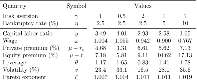
By Theorem 4.1, computing the equilibrium with positive consumption reduces to solving a single nonlinear equation (4.11). If the existence condition (4.10) fails, we need to look for an equilibrium with zero consumption, in which case we need to solve a system of two nonlinear equations (4.11) and (4.12). Table 1 shows the results, which are all equilibria with positive consumption. The pri-vate equity premium, leverage (fraction of own physical capital to entrepreneur net worth), and volatility are all reasonable numbers, roughly in line with U.S. stock returns. In each case, the upper tail Pareto exponent ζ is close to 1, in agreement with Zipf’s law.
As we make the environment riskier (largerγor η), the private equity pre-mium goes up, the capital-labor ratio goes down, which also suppresses the wage. However, the mechanism is very different depending on whether we increase risk aversion γ or the bankruptcy rateη. When γ increases, the entrepreneurs be-come less willing to invest capital, so they leverage less (portfolio effect). Since there is less investment in the high return capital, the aggregate capital goes down. On the other hand, when η increases, aggregate capital goes down just because there is more bankruptcy and hence destruction of capital (resource ef-fect). Since capital is more scarce, the risk premium goes up, and entrepreneurs leverage more to take advantage.
It is not surprising that the upper tail Pareto exponentζ is close to 1 re-gardless of the parameter specification. The reason is that, according to (3.11), we always have the bound
1< ζ <1 +2ηκ v2 .
21Aoki and Nirei (2017) also assumeγ= 1 (log utility), but the reason is for tractability
Table 1: Parameters and endogenous variables in steady state.
Quantity Symbol Values
Risk aversion γ 1 0.5 2 1 1
Bankruptcy rate (%) η 2.5 2.5 2.5 5 10
Capital-labor ratio y 3.49 4.01 2.93 2.58 1.65
Wage ω 1.004 1.055 0.942 0.900 0.767
Private premium (%) µ−re 4.68 3.31 6.61 5.62 7.13
Equity premium (%) µ−r 7.18 5.81 9.11 10.62 17.13
Leverage θ 1.17 1.65 0.83 1.41 1.78
Volatility (%) v 23.4 33.1 16.5 28.1 35.6
Pareto exponent ζ 1.007 1.004 1.011 1.011 1.019
Note: the table shows the values of endogenous variables in steady state. The capital-labor ratio isy =K/N, where Kis the aggregate capital. The private premium is the expected return on capital in excess of the effective risk-free rate faced by entrepreneurs,µ−re, where
µ= f′
(y) andre =r+η = ρW +η is the effective risk-free rate (true risk-free rate plus
spread). The equity premium is the expected return on capital in excess of the risk-free rate r=ρW conditional on survival. The leverageθ= µ
−re
γσ2 is the ratio between entrepreneur’s
own physical capital to net worth. v=σθis the volatility of entrepreneur’s net worth (which is also the market capitalization of the firm). ζis the upper tail Pareto exponent computed as in Theorem 3.5.
As a rough estimate, the bankruptcy rateηhas order of magnitude about 10−1
or 10−2 and the volatility v has order of magnitude about 10−1. Hence the
upper bound ofζis 1 +2vηκ2 ≈1 +κ. Sinceκis the ratio of the initial capital of new firms to that of the average firm, it is reasonable to expect thatκis quite small. Thereforeζmust be close to 1.
4.4.3 Sensitivity analysis
How robust is Zipf’s law? In this section, I conduct two robustness checks. First, I fix the parameter values (ρW, ρ, γ, ε, α, δ, σ, η, N) at the baseline
spec-ification and vary one parameter at a time up to ten-fold increase or decrease. (For the capital share α, I consider all values in (0,1).) For example, since at the baseline we haveγ= 1, I considerγ∈[0.1,10]. Figure 3 shows the results. We can see that in all cases the Pareto exponentζis slightly above 1 regardless of the parameter values (which can be quite extreme), and in most cases below 1.1, consistent with Zipf’s law.
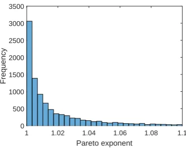
In the second robustness check, I generate 10,000 random parameter con-figurations and compute the Pareto exponent for each simulation. For this experiment, I consider up to five-fold changes in the parameters, so in each simulation a parameter is 5U times the baseline value, where U is uniformly
drawn from [−1,1] independently across all parameters and simulations. (For the capital shareα, it is uniformly drawn from [0.1α,1.9α].)
0 0.02 0.04 0.06 0.08 0.1 Worker discount rate (ρ
W) 1
1.05 1.1
0 0.1 0.2 0.3 0.4
Entrepreneur discount rate (ρ) 1
1.05 1.1
0 2 4 6 8 10
Relative Risk Aversion (γ) 1
1.05 1.1
0 2 4 6 8 10
Elasticity of Intertemporal Substitution (ǫ) 1
1.05 1.1
0 0.2 0.4 0.6 0.8 1
Capital share (α) 1
1.05 1.1
0 0.2 0.4 0.6 0.8
Capital depreciation rate (δ) 1
1.05 1.1
0 0.5 1 1.5 2
Capital volatility (σ) 1
1.05 1.1
0 0.05 0.1 0.15 0.2 0.25 Bankruptcy rate (η)
1 1.05 1.1
0 50 100 150 200
Average firm size (N) 1
[image:25.595.122.469.126.470.2]1.05 1.1
Figure 3: Sensitivity of Pareto exponent ζwith respect to model parameters.
Note: The figure plots the upper tail Pareto exponent ζcomputed as in Theorem 3.5. The dotted vertical lines indicate the baseline parameter values.
5
Concluding remarks
This paper shows that Zipf’s law (Pareto exponent slightly above 1) can be explained by embedding the standard random growth model into a general equilibrium model and introducing a factor of production that is mobile but in limited supply. Unlike existing explanations of Zipf’s law, my theory does not require a fine-tuning of parameters.
Pareto exponent
1 1.02 1.04 1.06 1.08 1.1
Frequency
[image:26.595.196.384.131.281.2]0 500 1000 1500 2000 2500 3000 3500
Figure 4: Histogram of Pareto exponent ζ with random parameter configura-tions.
knowledge-based activities relaxed this constraint thereafter. Since my theory requires that a factor of production is in limited supply but mobile, and land is clearly immobile, the failure of Zipf’s law before 1500 is entirely consistent with my theory.
A
Fokker-Planck equation
In this appendix, I explain theFokker-Planck equation, also known as the Kol-mogorov forward equation, which is useful in characterizing the cross-sectional distribution in general settings.
A.1
Fokker-Planck equation
Consider the diffusion
dXt=g(t, Xt) dt+v(t, Xt) dBt, (A.1)
whereBtis standard Brownian motion. Letp(x, t) be the density ofXtat time
t. Then
∂p ∂t =−
∂ ∂x(gp) +
1 2
∂2 ∂x2(v
2p), (A.2)
which is known as theFokker-Planck (Kolmogorov forward) equation.
The Fokker-Planck equation (A.2) holds if the diffusion (A.1) holds at all times. However, we can consider situations in which the process is occasionally reset. For example, ifXtin (A.1) describe individual wealth, since the individual
will die eventually, we need to specify what happens when an individual dies. If there is influxj+(x, t) and outfluxj−(x, t) per unit of time at locationxat timet, then the Fokker-Planck equation (A.2) must be modified as
∂p ∂t =−
∂ ∂x(gp) +
1 2
∂2 ∂x2(v
For example, if the units exit at constant probabilityηper unit of time (Poisson rateη) and enter at locationx0, then the FPE becomes
∂p ∂t =−
∂ ∂x(gp) +
1 2
∂2 ∂x2(v
2p) +ηδ(x
−x0)−ηp,
whereδ(x−x0) is the Dirac delta function located at x0.
A.2
Stationary density
If the diffusion has time-independent driftg(x) and variancev(x) and admits a stationary distributionp(x), then we get
0 =− d
dx(gp) + 1 2
d2
dx2(v 2p).
Integrating with respect toxand using the boundary conditionp(x), p′(x)→0 as x→ ±∞, we get
0 =−g(x)p(x) +1 2(v(x)
2p(x))′.
Lettingq(x) =v(x)2p(x) and solving the ODE, we get
q′ =2g v2q ⇐⇒
q′ q =
2g v2
⇐⇒ logq(x) =
Z q′(x)
q(x) dx=
Z 2g(x)
v(x)2dx
⇐⇒ q(x) = exp
Z 2g(x)
v(x)2 dx
.
Therefore the stationary density is
p(x) = q(x) v(x)2 =
1 v(x)2exp
Z 2g(x)
v(x)2 dx
, (A.3)
where the constant of integration is determined by the conditionR−∞∞ p(x) dx= 1 sincep(x) is a density.
If there is a constant probability of death η, the stationary density is the solution of the second-order ODE
0 =− d
dx(gp) + 1 2
d2
dx2(v 2p)
−ηp,
which holds at every point exceptx0.
A.2.1 Geometric Brownian motion with minimum size
As examples, consider the geometric Brownian motion with minimum sizexmin
or constant Poisson rateηof birth/death with reset sizex0. In the former case,
settingg(x) =gx(withg <0) andv(x) =vxin (A.3), the stationary density is
p(x) = 1 (vx)2exp
Z 2gx
(vx)2dx
for some constantC > 0. Since the minimum size is xmin and the probability
must add up to 1, it follows that
1 =C
Z ∞
xmin
xv2g2−2= C 1−2vg2
x−1+ 2g v2
min .
Therefore
p(x) =ζxζminx−ζ−1
for ζ= 1−2g/v2, which is the probability density function of the Pareto
dis-tribution (2.2) with exponentζ >1.
A.2.2 Geometric Brownian motion with Poisson entry/exit
Next, consider the geometric Brownian motion with entry/exit at Poisson rate η >0 and initial size x0. In this case, it is easier to solve in logs. Using Itˆo’s
lemma, Yt= logXtobeys the Brownian motion
dYt=
g−12v2
dt+vdBt.
The Fokker-Planck equation in the steady state is
0 =−
g−12v2
p′(y) +1 2v
2p′′(y)−ηp(y)
except aty0:= logx0, where I used the fact thatg, v are constant. Since this
is a linear second-order ODE with constant coefficients, the general solution is
p(y) =C1e−λ1y+C2e−λ2y,
whereλ1>0> λ2 are solutions to the quadratic equation
1 2v
2ξ2+
g−1
2v
2
ξ−η= 0,
which is (2.6). Since the PDF must be continuous, p(y)→0 asy → ±∞, and integrate to 1, lettingα=λ1>0 andβ=−λ2>0, it follows that
p(y) =
( αβ
α+βe−
α|y−y0|, (y≥y 0)
αβ α+βe−
β|y−y0|, (y≤y 0)
which is the asymmetric Laplace distribution with modey0and exponentsα, β.
Taking the exponential, we obtain the double Pareto distribution (2.5).
B
Proofs
Proof of Lemma 3.4. Suppose that a