A Unified Statistical Model for the Identification of English BaseNP

(1)

A Unified Statistical Model for the Identification of English

BaseNP

Endong Xun Microsoft Research China No. 49 Zhichun Road Haidian District

Ming Zhou Microsoft Research China No. 49 Zhichun Road Haidian District

Changning Huang Microsoft Research China No. 49 Zhichun Road Haidian District

Abstract

This paper presents a novel statistical model for automatic identification of English baseNP. It uses two steps: the N-best Part-Of-Speech (POS) tagging and baseNP identification given the N-best POS-sequences. Unlike the other approaches where the two steps are separated, we integrate them into a unified statistical framework. Our model also integrates lexical information. Finally, Viterbi algorithm is applied to make global search in the entire sentence, allowing us to obtain linear complexity for the entire process. Compared with other methods using the same testing set, our approach achieves 92.3% in precision and 93.2% in recall. The result is comparable with or better than the previously reported results.

1

Introduction

Finding simple and non-recursive base Noun Phrase (baseNP) is an important subtask for many natural language processing applications, such as partial parsing, information retrieval and machine translation. A baseNP is a simple noun phrase that does not contain other noun phrase recursively, for example, the elements within [...] in the following example are baseNPs, where NNS, IN VBG etc are part-of-speech tags [as defined in M. Marcus 1993].

[Measures/NNS] of/IN [manufacturing/VBG activity/NN] fell/VBD more/RBR than/IN

[the/DT overall/JJ measures/NNS] ./.

Figure 1: An example sentence with baseNP brackets

A number of researchers have dealt with the problem of baseNP identification (Church 1988; Bourigault 1992; Voutilainen 1993; Justeson & Katz 1995). Recently some researchers have made experiments with the same test corpus extracted from the 20th section of the Penn Treebank Wall Street Journal (Penn Treebank). Ramshaw & Markus (1998) applied transform-based error-driven algorithm (Brill 1995) to learn a set of transformation rules, and using those rules to locally updates the bracket positions. Argamon, Dagan & Krymolowski (1998) introduced a memory-based sequences learning method, the training examples are stored and generalization is performed at application time by comparing subsequence of the new text to positive and negative evidence. Cardie & Pierce (1998 1999) devised error driven pruning approach trained on Penn Treebank. It extracts baseNP rules from the training corpus and prune some bad baseNP by incremental training, and then apply the pruned rules to identify baseNP through maximum length matching (or dynamic program algorithm).

(2)

two steps together such that the final output takes the uncertainty in both steps together. The approaches proposed by Ramshaw & Markus and Cardie&Pierce are deterministic and local, while Argamon, Dagan & Krymolowski consider the problem globally and assigned a score to each possible baseNP structures. However, they did not consider any lexical information.

This paper presents a novel statistical approach to baseNP identification, which considers both steps together within a unified statistical framework. It also takes lexical information into account. In addition, in order to make the best choice for the entire sentence, Viterbi algorithm is applied. Our tests with the Penn Treebank showed that our integrated approach achieves 92.3% in precision and 93.2% in recall. The result is comparable or better that the current state of the art.

In the following sections, we will describe the detail for the algorithm, parameter estimation and search algorithms in section 2. The experiment results are given in section 3. In section 4 we make further analysis and comparison. In the final section we give some conclusions.

2

The statistical approach

In this section, we will describe the two-pass statistical model, parameters training and Viterbi algorithm for the search of the best sequences of POS tagging and baseNP identification. Before describing our algorithm, we introduce some notations we will use

2.1 Notation

Let us express an input sentence E as a word sequence and a sequence of POS respectively as follows:

n

w

E

=

1 2

...

−1

n n

t

T

=

1 2

...

−1

Where

n

is the number of words in the sentence,

t

i is the POS tag of the word

w

i.

Given E, the result of the baseNP identification is assumed to be a sequence, in which some words are grouped into baseNP as follows

... ]

... [

...wi−1 wi wi+1 wj wj+1 The corresponding tag sequence is as follows:

(a)

m j

j i i j j i i

i t t t t t b t n n n t

B=...−1 [ +1 ...] +1... =...−1 , +1 ...=1 2 ...

In which

b

_i_,_j corresponds to the tag sequence of

a baseNP: [ti ti+1... tj].

b

i,j may also be

thought of as a baseNP rule. Therefore B is a sequence of both POS tags and baseNP rules. Thus 1≤m≤n, n_i∈(POS tag set∪ baseNP rules set), This is the first expression of a sentence with baseNP annotated. Sometime, we also use the following equivalent form:

(b)

n j

j j j i i i i i

i bm tbm t bm tbm t bm q q q

t

Q=...(−1, −1) (, ) (+1, +1)...(, ) (+1, +1)...= 1 2...

Where each POS tag

t

_i is associated with its

positional information

bm

_i with respect to

baseNPs. The positional information is one of }

, , , ,

{F I E O S . F, E and I mean respectively that the word is the left boundary, right boundary of a baseNP, or at another position inside a baseNP. O means that the word is outside a baseNP. S marks a single word baseNP. This second expression is similar to that used in [Marcus 1995].

For example, the two expressions of the example given in Figure 1 are as follows:

(a) B= [NNS] IN [VBG NN] VBD RBR IN [DT JJ NNS]

(b) Q=(NNS S) (IN O) (VBG F) (NN E) (VBD O) (RBR O) (IN O) (DT F) (JJ I) (NNS E) (. O)

2.2 An

‘integrated’ two-pass

procedure

The principle of our approach is as follows. The most probable baseNP sequence

B

* may be expressed generally as follows:

))

|

(

max

arg

*

E

B

p

B

=

We separate the whole procedure into two passes, i.e.:

)) , | ( ) | ( ( max arg

*

E T B P E T P B

B

×

≈ (1)

In order to reduce the search space and computational complexity, we only consider the N best POS tagging of E, i.e.

))

|

(

max

arg

)

(

,..., 1

E

T

P

best

N

T

N

T T T=

=

−

(2)

Therefore, we have:

))

,

|

(

)

|

(

max

arg

,..., , *

1

E

T

B

P

E

T

P

B

N

T T T B

×

≈

(3)

Correspondingly, the algorithm is composed of two steps: determining the N-best POS tagging using Equation (2). And then determining the best baseNP sequence from those POS sequences using Equation (3). One can see that the two steps are integrated together, rather that separated as in the other approaches. Let us now examine the two steps more closely.

2.3 Determining the N best POS

sequences

The goal of the algorithm in the 1st pass is to search for the N-best POS-sequences within the

search space (POS lattice). According to Bayes’ Rule, we have

)

(

)

(

)

|

(

)

|

(

E

P

T

P

T

E

P

E

T

P

=

×

Since

P

(E

)

does not affect the maximizing

procedure of

P

(

T

|

E

)

, equation (2) becomes

)) ( ) | ( ( max arg )) | ( ( max arg ) ( ,..., ,..., 1 1 T P T E P E T P best N T N

N TT T

T T T × = = − = = (4)

We now assume that the words in E are independent. Thus

∏

=

≈

n i i i

t

w

P

T

E

P

1

)

|

(

)

|

(

(5)

We then use a trigram model as an approximation of P(T), i.e.:

∏

= − −

≈

n i i i

i

t

P

T

P

1 1 2

,

)

|

(

)

(

(6)

Finally we have

))

|

(

max

arg

)

(

,..., 1

E

T

P

best

N

T

N T T T=

=

−

))

,

|

(

)

|

(

max

arg

₂ ₁

1 ,..., 1 − − = =

×

=

∏

i i i

n i i i T T T

t

P

t

w

P

N (7)

In Viterbi algorithm of N best search,

P

(

w

_i

|

t

_i

)

is called lexical generation (or output) probability, and

P

(

t

_i

|

t

_i₋₂

,

t

_i₋₁

)

is called

transition probability in Hidden Markov Model.

2.3.1 Determining the baseNPs

As mentioned before, the goal of the 2nd pass is to search the best baseNP-sequence given the N-best POS-sequences.

Considering E,T and Bas random variables, according to Bayes’ Rule, we have

)

|

(

)

,

|

(

)

|

(

)

,

|

(

T

E

P

T

B

E

P

T

B

P

E

T

B

P

=

×

Since ) ( ) ( ) | ( ) | ( T P B P B T P T B

P = × we have,

) ( ) | ( ) ( ) | ( ) , | ( ) , | ( T P T E P B P B T P T B E P E T B P × × ×

= (8)

Because we search for the best baseNP sequence for each possible POS-sequence of the given

sentence E, so

const T E P T P T E

P( | )× ( )= ( ∩ )= ,

Furthermore from the definition of B, during

each search procedure, we have

∏

= = = n i j i j i t b t P B T P 1

,) 1

| ,..., ( ) |

( . Therefore, equation

(3) becomes )) , | ( ) | ( ( max arg ,..., , * 1 E T B P E T P B N T T T B × = = )) ( ) , | ( ) | ( ( max arg ,..., , 1 B P T B E P E T P N T T T B × × = = (9)

using the independence assumption, we have

∏

=

≈

n i i i i

t

bm

w

P

T

B

E

P

1

)

,

|

(

)

,

|

(

(10)

With trigram approximation of

P

(B

)

, we have:

∏

= − −

≈

m i i i

i

n

P

B

P

1 1 2

,

)

|

(

)

(

(11)

Finally, we obtain

) ) , | ( ) , | ( ) | ( ( max arg , 1 1 2 1 ,.. , * 1

∏

= − − = = × × = m i i i i n i i i i T T T B n n n P t bm w P E T P B N 12

To summarize, In the first step, Viterbi N-best searching algorithm is applied in the POS tagging procedure, It determines a path probability

f

_t for each POS sequence calculated

as follows:

∏

= − −

×

=

n i i i i i i

t

p

w

t

p

t

f

, 1

1 2

,

)

|

(

)

|

(

.

In the second step, for each possible POS tagging result, Viterbi algorithm is applied again to search for the best baseNP sequence. Every baseNP sequence found in this pass is also asssociated with a path probability

∏

= − − =

×

=

m i i i i n i i i i

b

p

w

t

bm

p

n

f

, 1 1 2 1

)

,

|

(

)

,

|

(

.

The integrated probability of a baseNP sequence

is determined by

f

t

×

f

b α

(4)

normalization coefficient (

α

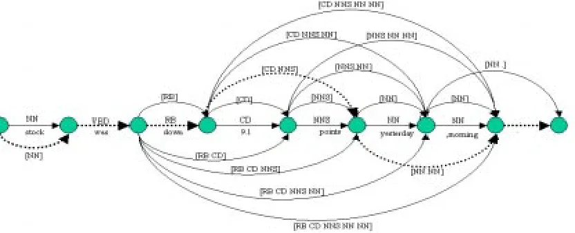
=2.4 in our experiments). When we determine the best baseNP sequence for the given sentenceE, we also determine the best POS sequence of E, which corresponds to the best baseNP of E. Now let us illustrate the whole process through an example: “stock was down 9.1 points yesterday morning.”. In the first pass, one of the

N-best POS tagging result of the sentence is: T = NN VBD RB CD NNS NN NN. For this POS sequence, the 2nd pass will try to determine the baseNPs as shown in Figure 2. The details of the path in the dash line are given in Figure 3, Its probability calculated in the second pass is as follows (

Φ

is pseudo variable):

) , | (

) , | ( ) , | ( ) , | ( ) , |

(B T E p stock NN S p was VBD O p down RB O p NUMBER CD B

P = × × ×

) ., | (. ) , | (

) , | (

) , | int

(po s NNS E p yesterday NN B p morning NN E p O

p × × ×

×

) , | ] ([

) ], [ | ( ]) [ , | ( ) , | ]

([NN pVBD NN p RB NN VBD p CD NNS VBD RB

p Φ Φ × Φ × ×

×

])

[

],

[

|

(.

])

[

,

|

]

([

NN

RB

CD

NNS

p

CD

NNS

NN

p

×

[image:4.595.87.503.303.472.2]

×

[image:4.595.72.501.523.605.2]

Figure 2: All possible brackets of "stock was down 9.1 points yesterday morning"

Figure 3: the transformed form of the path with dash line for the second pass processing

2.4 The statistical parameter

training

In this work, the training and testing data were derived from the 25 sections of Penn Treebank. We divided the whole Penn Treebank data into two sections, one for training and the other for testing.

As required in our statistical model, we have to calculate the following four probabilities: (1)P(t_i |t_i₋₂,t_i₋₁), (2)

P

(

w

i

|

t

i

)

, (3)

P

(

n

i

|

n

i−2

n

i−1

)

and (4)

P

(

w

i

|

t

i

,

bm

i

)

. The

(5)

(1) and (2) can be calculated from POS tagged data with following formulae:

∑

− −

− − −

− =

j

j i i

i i i i

i i

t t t count

t t t count t

t t p

) (

) , | (

1 2

1 2 1

2 (13)

)

(

)

(

)

|

(

i

i i

t

count

t

tag

with

w

count

t

w

p

=

(14)

As each sentence in the training set has both POS tags and baseNP boundary tags, it can be converted to the two sequences as B (a) and Q (b) described in the last section. Using these sequences, parameters (3) and (4) can be calculated, The calculation formulas are similar with equations (13) and (14) respectively. Before training trigram model (3), all possible baseNP rules should be extracted from the training corpus. For instance, the following three sequences are among the baseNP rules extracted.

There are more than 6,000 baseNP rules in the Penn Treebank. When training trigram model (3), we treat those baseNP rules in two ways. (1) Each baseNP rule is assigned a unique identifier (UID). This means that the algorithm considers the corresponding structure of each baseNP rule. (2) All of those rules are assigned to the same identifier (SID). In this case, those rules are grouped into the same class. Nevertheless, the identifiers of baseNP rules are still different from the identifiers assigned to POS tags. We used the approach of Katz (Katz.1987) for parameter smoothing, and build a trigram model to predict the probabilities of parameter (1) and (3). In the case that unknown words are encountered during baseNP identification, we calculate parameter (2) and (4) in the following way:

2 )) , ( ( max

) , ( )

, | (

i j j

i i i

i i

t bm count

t bm count t

bm w

p = (15)

2

))

(

max

)

(

)

|

(

j j

i i

i

t

count

t

count

t

w

p

=

(16)

Here, bm_j indicates all possible baseNP labels

attached to

t

_i, and t_j is a POS tag guessed for

the unknown word

w

_i.

3

Experiment result

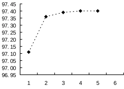
We designed five experiments as shown in Table 1. “UID” and “SID” mean respectively that an identifier is assigned to each baseNP rule or the same identifier is assigned to all the baseNP rules. “+1” and “+4” denote the number of beat POS sequences retained in the first step. And “UID+R” means the POS tagging result of the given sentence is totally correct for the 2nd step. This provides an ideal upper bound for the system. The reason why we choose N=4 for the N-best POS tagging can be explained in Figure 4, which shows how the precision of POS tagging changes with the number N.

96. 95 97. 00 97. 05 97. 10 97. 15 97. 20 97. 25 97. 30 97. 35 97. 40 97. 45

[image:5.595.318.531.434.587.2]

1 2 3 4 5 6

Figure 4: POS tagging precision with respect to different number of N-best

In the experiments, the training and testing sets are derived from the 25 sections of Wall Street Journal distributed with the Penn Treebank II, and the definition of baseNP is the same as

Ramshaw’s, Table 1 summarizes the average

performance on both baseNP tagging and POS tagging, each section of the whole Penn Treebank was used as the testing data and the other 24 sections as the training data, in this way

(6)

Precision ( baseNP %)

Recall ( baseNP %)

F-Measure

( baseNP %) 2

R P+

( baseNP %)

Precision (POS %)

UID+1 92.75 93.30 93.02 93.02 97.06

UID+4 92.80 93.33 93.07 93.06 97.02

SID+1 86.99 90.14 88.54 88.56 97.06

SID+4 86.99 90.16 88.55 88.58 97.13

UID+R 93.44 93.95 93.69 93.70 100

Table 1 The average performance of the five experiments

88. 00 88. 50 89. 00 89. 50 90. 00 90. 50 91. 00 91. 50 92. 00 92. 50 93. 00

1 2 3 4 5 6

[image:6.595.161.522.105.392.2]

UI D+1 UI D+4 UI D+R

Figure 5: Precision under different training sets and different POS tagging results

91. 60 91. 80 92. 00 92. 20 92. 40 92. 60 92. 80 93. 00 93. 20 93. 40 93. 60

1 2 3 4 5 6

[image:6.595.87.375.109.392.2]

UI D+1 UI D+4 UI D+R

Figure 6: Recall under different training sets and different POS tagging results

96. 80 96. 85 96. 90 96. 95 97. 00 97. 05 97. 10 97. 15 97. 20

1 2 3 4 5 6

Vi t er bi UI D+4 SI D+4

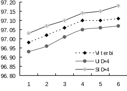
Figure 7: POS tagging precision under different training sets

Figure 5 -7 summarize the outcomes of our statistical model on various size of the training data, x-coordinate denotes the size of the training set, where "1" indicates that the training set is from section 0-8th of Penn Treebank, "2" corresponds to the corpus that add additional three sections 9-11th into "1" and so on. In this

way the size of the training data becomes larger and larger. In those cases the testing data is always section 20 (which is excluded from the training data).

[image:6.595.317.529.240.387.2] [image:6.595.82.292.454.605.2]

(7)

4

Comparison with other

approaches

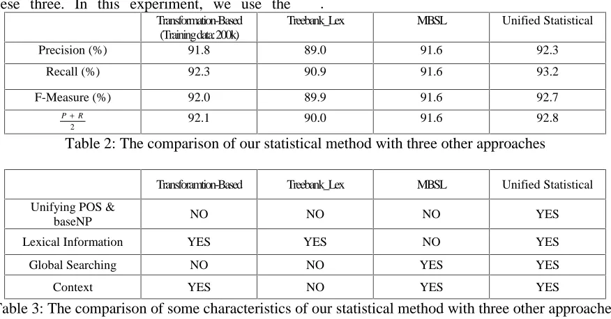
To our knowledge, three other approaches to baseNP identification have been evaluated using Penn Treebank-Ramshaw & Marcus’s transformation-based chunker, Argamon et al.’s MBSL, and Cardie’s Treebank_lex in Table 2, we give a comparison of our method with other these three. In this experiment, we use the

testing data prepared by Ramshaw (available at http://www.cs.biu.ac.il/~yuvalk/MBSL), the training data is selected from the 24 sections of Penn Treebank (excluding the section 20). We can see that our method achieves better result than the others

.

Transformation-Based (Training data: 200k)

Treebank_Lex MBSL Unified Statistical

Precision (%) 91.8 89.0 91.6 92.3 Recall (%) 92.3 90.9 91.6 93.2 F-Measure (%) 92.0 89.9 91.6 92.7

2 R

P+ _92.1 _90.0 _91.6 _92.8

Table 2: The comparison of our statistical method with three other approaches

Transforamtion-Based Treebank_Lex MBSL Unified Statistical Unifying POS &

baseNP NO NO NO YES

[image:7.595.79.517.203.432.2]

Lexical Information YES YES NO YES Global Searching NO NO YES YES Context YES NO YES YES

Table 3: The comparison of some characteristics of our statistical method with three other approaches

Table 3 summarizes some interesting aspects of our approach and the three other methods. Our statistical model unifies baseNP identification and POS tagging through tracing N-best sequences of POS tagging in the pass of baseNP recognition, while other methods use POS tagging as a pre-processing procedure. From Table 1, if we reviewed 4 best output of POS tagging, rather that only one, the F-measure of baseNP identification is improved from 93.02 % to 93.07%. After considering baseNP information, the error ratio of POS tagging is reduced by 2.4% (comparing SID+4 with SID+1).

The transformation-based method (R&M 95) identifies baseNP within a local windows of sentence by matching transformation rules. Similarly to MBSL, the 2nd pass of our algorithm traces all possible baseNP brackets, and makes global decision through Viterbi searching. On the other hand, unlike MSBL we take lexical information into account. The experiments show that lexical information is very helpful to improve both precision and recall of baseNP

recognition. If we neglect the probability of

∏

=

n

i

i i i t bm w

P 1

) , |

( in the 2nd pass of our model,

the precision/recall ratios are reduced to 90.0/92.4% from 92.3/93.2%. Cardie’s approach to Treebank rule pruning may be regarded as the special case of our statistical model, since the maximum-matching algorithm of baseNP rules is only a simplified processing version of our statistical model. Compared with this rule pruning method, all baseNP rules are kept in our model. Therefore in principle we have less likelihood of failing to recognize baseNP types As to the complexity of algorithm, our approach is determined by the Viterbi algorithm approach, or

O

(n

)

, linear with the length.

5

Conclusions

(8)

(1) baseNP identification is implemented in two related stages: N-best POS taggings are first determined, then baseNPs are identified given the N best POS-sequences. Unlike other approaches that use POS tagging as pre-processing, our approach is not dependant on perfect POS-tagging, Moreover, we can apply baseNP information to further increase the precision of POS tagging can be improved. These experiments triggered an interesting future research challenge: how to cluster certain baseNP rules into certain identifiers so as to improve the precision of both baseNP and POS tagging. This is one of our further research topics.

(2) Our statistical model makes use of more lexical information than other approaches. Every word in the sentence is taken into account during baseNP identification.

(3) Viterbi algorithm is applied to make global search at the sentence level.

Experiment with the same testing data used by the other methods showed that the precision is 92.3% and the recall is 93.2%. To our knowledge, these results are comparable with or better than all previously reported results.

References

Eric Brill and Grace Ngai. (1999) Man vs. machine: A case study in baseNP learning. In Proceedings of the 18th

International Conference on Computational Linguistics, pp.65-72. ACL’99

S. Argamon, I. Dagan, and Y. Krymolowski (1998) A memory-based approach to learning shallow language patterns. In Proceedings of the 17th

International Conference on Computational Linguistics, pp.67-73. COLING-ACL’98

Cardie and D. Pierce (1998) Error-driven pruning of treebank grammas for baseNP identification. In Proceedings of the 36th

International Conference on Computational Linguistics, pp.218-224. COLING-ACL’98

Lance A. Ramshaw and Michael P. Marcus ( In Press). Text chunking using transformation-based learning. In Natural Language Processing Using Very large Corpora. Kluwer. Originally appeared in The second workshop on very large corpora WVLC’95, pp.82-94.

Viterbi, A.J. (1967) Error bounds for convolution codes and asymptotically optimum decoding algorithm. IEEE Transactions on Information Theory IT-13(2): pp.260-269, April, 1967

S.M. Katz.(1987) Estimation of probabilities from sparse data for the language model component of speech recognize. IEEE Transactions on Acoustics, Speech and Signal Processing. Volume ASSP-35, pp.400-401, March 1987

Church, Kenneth. (1988) A stochastic parts program and noun phrase parser for unrestricted text. In Proceedings of the Second Conference on Applied Natural Language Processing, pages 136-143. Association of Computational Linguistics.