Everything you always wanted to know about bitcoin modelling but were afraid to ask

Munich Personal RePEc Archive

Everything you always wanted to know

about bitcoin modelling but were afraid

to ask

Fantazzini, Dean and Nigmatullin, Erik and Sukhanovskaya,

Vera and Ivliev, Sergey

Moscow School of Economics - Moscow State University, Bocconi

University, Milan (Italy), Perm State National Research University;

Laboratory of Crypto-Economics and Blockchain systems, Perm

State National Research University; Laboratory of

Crypto-Economics and Blockchain systems

2016

Online at

https://mpra.ub.uni-muenchen.de/71946/

Everything you always wanted to know about bitcoin modelling

but were afraid to ask

Dean Fantazzini

Erik Nigmatullin

Vera Sukhanovskaya

Sergey Ivliev

Abstract

Bitcoin is an open source decentralized digital currency and a payment system. It has raised a lot of attention and interest worldwide and an increasing number of articles are devoted to its operation, economics and financial viability. This article reviews the econometric and mathematical tools which have been proposed so far to model the bitcoin price and several related issues, highlighting advan-tages and limits. We discuss the methods employed to determine the main characteristics of bitcoin users, the models proposed to assess the bitcoin fundamental value, the econometric approaches sug-gested to model bitcoin price dynamics, the tests used for detecting the existence of financial bubbles in bitcoin prices and the methodologies suggested to study the price discovery at bitcoin exchanges.

Keywords: Bitcoin, Crypto-currencies, Hash rate, Investors’ attractiveness, Social interactions, Money supply, Money Demand, Speculation, Forecasting, Algorithmic trading, Bubble, Price discov-ery.

JEL classification: C22, C32, C51, C53, E41, E42, E47, E51, G17.

Applied Econometrics

, forthcoming

∗_{Moscow School of Economics, Moscow State University, Leninskie Gory, 1, Building 61, 119992, Moscow, Russia. Fax:} +7 4955105256 . Phone: +7 4955105267 . E-mail: fantazzini@mse-msu.ru.

†_{Bocconi University, Milan (Italy); nigmatullin.erik@gmail.com}

‡_{Perm State National Research University; Laboratory of Crypto-Economics and Blockchain systems;}

vera-sukhanovskaya@yandex.ru

§_{Perm State National Research University; Laboratory of Crypto-economics and Blockchain systems; ivliev@gmail.com.}

1

Introduction

Bitcoin is an online decentralized currency that allows users to buy goods and services and execute transactions, without involving third parties. It was launched in 2009 by a person or (more likely) by a group of people operating under the name of Satoshi Nakamoto. Bitcoin belongs to the large family of “cryptocurrencies”, which are based on cryptographic methods of protection. The main characteristic of these currencies is their decentralized structure: there is no central authority which issues and regu-lates the currency, and transactions are executed using a peer-to-peer crypto-currency protocol without intermediaries. Introductory surveys about bitcoin structure and operation can be found in Becker et al. (2013), Segendorf (2014), Dwyer (2014), B¨ohme et al. (2015), or simply in Bitcoin (2015). Several central banks also examined bitcoin, see Velde (2013), Lo and Wang (2014), Baden and Chen (2014), Ali et al. (2014), and ECB (2012, 2015). Discussions of bitcoin as a potential alternative monetary system can be found in Rogojanu and Badea (2014) and Weber (2016), while the economics of bitcoin mining are examined in Kroll (2013). Analyses of the legal issues involved by using bitcoin can be found in Allen (2015) and Murphy et al. (2015).

The goal of this article is to review the econometric and mathematical tools which have been proposed so far to model the bitcoin price and several related issues. To our knowledge, such a review is missing in the financial literature and it can be of interest to both market professionals and researchers alike, given the early stages of the empirical literature devoted to bitcoin.

2

Definition of Crypto-currencies and Bitcoin

2.1

How Bitcoin works

2.1.1 Digital signatures and cryptographic hash function

The Bitcoin network uses cryptography to validate transactions during the payment processing and create transaction blocks. In particular, Bitcoin relies on two cryptographic schemes: 1) digital signatures and 2) a cryptographic hash function. The first scheme allows the exchange of payment instructions between the involved parties, while the second is used to maintain the discipline when recording transactions to the public ledger (known as Blockchain). It should be noted that none of these schemes is unique to Bitcoin, since they are widely used to protect commercial and government communications. A short description of how the Bitcoin network works is reported below, while more details can be found in Becker et al. (2013), Segendorf (2014), Dwyer (2014), B¨ohme et al. (2015), or simply in Bitcoin (2015). Digital signatures are used to authenticate digital messages between a sender and a recipient, and they provide:

(i) Authentication: the receiver can verify that the message came from the sender;

(ii) Non-repudiation: the sender cannot deny having sent the message;

(iii) Integrity: the message was not altered in transit.

The use of digital signatures includes public key cryptography, where a pair of keys (open and private) are generated with certain desirable properties. A digital signature is used for signing messages: the transaction is signed using a private key, and then transferred to the Bitcoin network. All the members of the network can verify that the transaction came from the owner of the public key, by taking the message, the signature, the public key and by running a test algorithm.

A cryptographic hash function takes as input a string of arbitrary length (the messagem), and returns the string with predetermined length (the hashh). The function is deterministic, which means that the same inputmwill always give the same outputh. In addition,the function must also have the following properties:

(i) Pre-image resistance: for a given hashh, it is difficult to find a messagemsuch that hash(m) =h

(ii) Collision resistance: for a given messagem1it is hard to find another messagem2 such that hash

(m1) = hash (m2). In other words, a change in the message leads to a change in the hash.

designed by the National Security Agency and published by the National Institute of Standards and Technology, see Dang (2012) for details.

2.1.2 Possession of bitcoins and bitcoin addresses

From a technical standpoint, bitcoins stay in the Bitcoin network on bitcoin-addresses. The ownership of a certain number of bitcoins is represented by the ability to send payments via the Bitcoin network using the bitcoins attached to these addresses. The ability to send payments to other bitcoin addresses is controlled by a digital signature, which include a public key and a private key. In particular, every bitcoin address is indexed by a unique public ID, which is an alphanumeric identifier, which corresponds to the public key. The private key controls the bitcoins stored at that address. Any payment (i.e. a

message) which involved this address as the sending address must be signed by the corresponding private key to be valid. In straight terms, the possession of bitcoins at a specified bitcoin address is given by the knowledge of the private key corresponding to that address.

At any point in time, every bitcoin address is associated with a bitcoin balance, which is public information. Each existing or proposed (broadcasted) transaction can be checked for compliance with the past transaction history, i.e. it is possible to verify that the transferred bitcoin do exist at the corresponding bitcoin address.

2.1.3 A transaction in the block chain

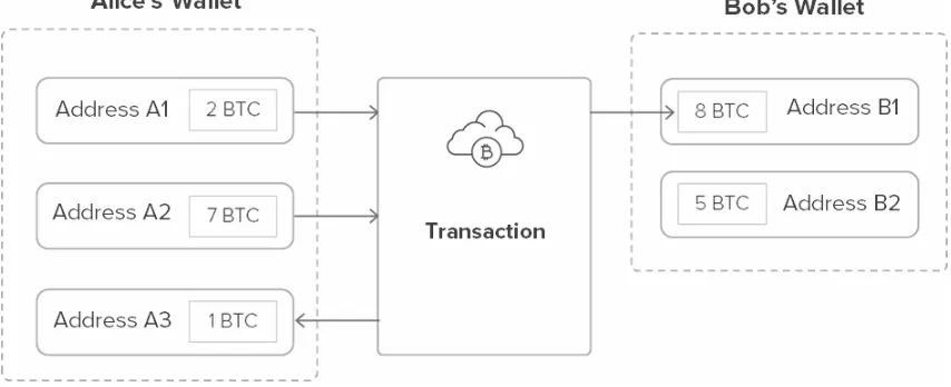
The agents who process transactions in the Bitcoin network use a set of bitcoin addresses calledwallet, which is the set of bitcoin addresses that belong to a single person/entity. Each transaction record includes one or more sending addresses (inputs) and one or more receiving addresses (outputs), as well as the information about how much each of these addresses sent and received. An example of a typical transaction is shown in Fig. 1.

In the example Alisa sends to Bob an amount of 8 BTC. This transactions has two inputs (2 and 7 BTC) and two outputs (8 and 1 BTC), where the transaction involving 1 BTC can be considered essentially as the change of the transaction, which is returned back to Alice. Since each transaction can have multiple sending addresses and receiving addresses, it is often impossible to link a specific sending address to a specific receiving address. The consequence of this is that you cannot assign a serial number to a specific bitcoin and trace its path in the Bitcoin network.

Figure 1: A typical transaction in the Bitcoin network

transactions in a [Bitcoin network] block; (d) multiple nodes cross-check each recorded transaction.

2.1.4 Starting a transaction

Suppose Alice wants to send Bob 1 bitcoin using the Bitcoin network. To do this, Alice and Bob must have a bitcoin address. Let’s call them ID Alice and ID Bob. Then, Alice needs to send and digitally certify the authenticity of the message, of this type

“ID Alice sends ID Bob 1 bitcoin.”

After Alice signs the transaction message with her private key and sends it, any participant in the Bitcoin network can verify Alice sent the message, and the message has not been altered. Moreover, as we discussed earlier, the digital signature guarantees that no one else could sign the message, so that Alice cannot deny that it has signed the message.

2.1.5 Checking a transaction

Before executing a transaction, the Bitcoin protocol must verify two aspects of the communication: first, whether it was Alice who sent the message. The digital signature scheme ensures that only the owner of the private key for that address may sign a message; secondly, to check whether there are sufficient funds in the address to ensure the completion of the transaction.

2.1.6 Updating the Blockchain

After the initial check of the transaction signed messages, validation nodes in the Bitcoin network begin to compete for the opportunity to record a transaction in the Blockchain. First, in the block of the transaction, competing nodes start putting together transactions, which were executed since the last record in the Blockchain. Then, the block is used to define a complex computing task. The node that first solves this task proceeds to record the transactions on the Blockchain and collects a reward.

The task which the competing nodes try to solve is based on one of the encryption schemes described above - the hash function. First, the block of the newly broadcasted transactions is again used as input for a cryptographic hash function to obtain a hash calleddigest. This digest, together with a one-time random code nounce (that is an alphanumeric string) and the hash of the previous block are used in another hash function that produces the hash of the Blockchain for the new block. The problem that the nodes have to solve includes finding such a random code, so that the hash of the new Blockchain has certain properties (in this case has a number of initial zeros). The first of the competing nodes which will find the right random code, transfers this information to the other participants in the network, and the Blockchain is updated. The implementation of this scheme is the so-called Hashcash - a proof that the system is operating properly (proof-of-work), and whose aim is to ensure that the computers use a certain amount of computing power to perform a task (see Beck (2002) for more details).

The nodes that perform the process of the proof-of-work in the Bitcoin network are called miners. These miners use their computing resources in this process with the goal to obtain the reward offered by the Bitcoin Protocol. Usually the reward is a predetermined number of newly created bitcoins. The rest of the reward (which is currently much smaller), is a voluntary transaction fee paid by those executing the transaction to the miners for transaction processing. The initial idea was that these voluntary contributions would replace the predetermined compensation of newly created bitcoins when this amount will tend to zero over time and a new incentive will be needed to stimulate the miners to process the transactions in the Bitcoin network (see Nakamoto (2009) for details).

2.2

Statistics of the Bitcoin network

2.2.1 Capitalization

The value of a digital currency is highly dependent on the number of participants, which in turn attracts more participants, powering a network effect. Therefore, bitcoin enjoys a significant first-mover advantage which has three aspects:

• the more users it has, the more useful Bitcoin becomes: there are more places where you can spend bitcoins, and business partners with whom you can exchange bitcoins, which in turns attracts more users;

• currencies require trust, but it can only be obtained over time, so that, ceteris paribus, the oldest currency has a natural advantage over competitors;

• the greater the volume, the higher the transaction fees, which attracts more miners and makes the network more secure, which in turn again attracts more users and traded funds.

With currencies that serve as a store of wealth, there is an additional lock-in effect as it is takes effort to transfer that wealth into other currencies. Thus, there are multiple effects in place that makes it very hard to dethrone Bitcoin. At this point in time, Bitcoin is the strongest leader among crypto currencies.

Figure 2: Market price of 1 Bitcoin in US dollars (2009-2016)

2.2.2 Network power

The value of the miners’ hardware exceeds $ 300 million, while the total computing power supporting the

Bitcoin network is approximately 800 Peta-hashes/s (see Fig. 3).

Figure 3: Computing power in the Bitcoin network: 01.01.2009 - 31.12.2015

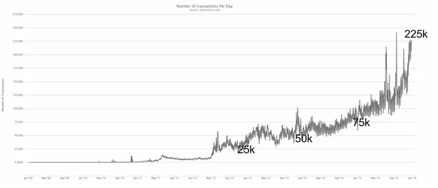
Figure 4: Number of transactions in the Bitcoin network: 01.01.2009 - 31.12.2015

3

Who uses Bitcoin? A review of econometric analysis of

Bit-coin users

The Bitcoin system has attracted attention worldwide and the number of scientific papers devoted to it is steadily increasing, see Bohme et al. (2015) and https://en.bitcoin.it/wiki/Research for more details. Unfortunately, a very limited number of studies has been devoted to the analysis of the characteristics of Bitcoin users, which could give a better understanding of this phenomenon and its future perspectives. The relative scarcity of academic interest in this field should not come as a surprise, given the extreme difficulty to gather data about Bitcoin users, who mostly want to remain anonymous. A couple of works tried to overcome this problem by interviewing a dozen of Bitcoin users, see Baur et al. (2015) and Huhtinen (2014).

Bohr and Bashir (2014) were the first to analyze a larger structured dataset, consisting of a survey conducted in 2013 by L´u´ı Smyth, at that time a digital anthropology researcher at the University College London. This survey consists of 1193 responses collected from February 12, 2013 through April 4, 2013. Bohr and Bashir (2014) tried to answer three research questions:1) what predicts the accumulation of wealth among Bitcoin users; 2) what predicts optimism about the near- and long-term value of Bitcoin; 3) what attracts people to Bitcoin. The first issue was examined by performing a simple regression of the self-reported amount of bitcoins owned (transformed to their log base 2 values to avoid skewness) against a set of Bitcoin users’ characteristics extracted from the survey:

• the user Age and the userAge squared to account for nonlinearity;

• a variable named “Installation”, which refers to when respondents first downloaded the Bitcoin client (software that connects to the Bitcoin network), and ranges from 1 = the first quarter of 2009 to 17 = the first quarter of 2013, and which is then centered on the mean;

• a dummy variable named “Miner” to account for whether or not individuals had ever gone through the process mining bitcoins themselves;

• an interaction term “Installation xMiner”, to test whether early Bitcoin miners obtained a large advantage in Bitcoin accumulation versus late adopters of Bitcoin;

• a dummy variables named “Bitcoin sins”, which is 1 if the respondent admitted to mining bitcoins through someone else’s hardware without their permission (via malware), or to steal someone else’s bitcoins;

• a dummy variables named “Illicit goods”, which is 1 if the respondent admitted to purchasing narcotics, gambling services, or other illicit goods with their bitcoins.

• a dummy variables named “Bitcoin talk”, which is 1 if the respondent indicated that he/she uses Bitcoin-specific platforms to talk with others about Bitcoin;

• a dummy variables named “Investor” , which is 1 if the respondent self-described their role within the context of Bitcoin as an investor.

• integer variables named “profit” and “community” ranging from 1 = not motivating to 5 =very motivating, for whether the respondents considered profit or community as motivating factors for their initial involvement with Bitcoin

Bohr and Bashir (2014) found that age was a statistically significant factor in predicting the amount of bitcoin a respondent held: young respondents hold fewer bitcoins, but the amount approximately double every 10 years reaching a maximum between 55 and 60 years old, similarly to accumulation across other asset classes. The interaction term Installationcdot Miner is significant, confirming that mining bitcoins was easier during the early days of its operation, so that early adopter miners gained an advantage in Bitcoin accumulation. Those who actively participated in bitcoin online communities owned twice as much bitcoin as those who do not, while those users who self-identified themselves as investors had accumulated about four times as many bitcoins as those who did not. Ceteris paribus, Bitcoin users who purchased illicit goods, such as narcotics, had up to 45% more bitcoin holdings than those who bought only legal goods

Bohr and Bashir (2014) then performed two additional regressions, where the near-term (four months from time of survey) and the long-term (six years from time of survey) expected values of one bitcoin in USD where regressed against the previous set of variables: older users were found to be less optimistic than younger users, with optimism peaking at about age 35, while the higher is the level of social engagement on online forums, the higher the predicted price. Interestingly, the later Bitcoin installers were more optimistic about the near-term value, while miners were more pessimistic than non-miners regarding the long-term value of Bitcoin.

politically as greens. Finally, users who like bitcoin for its freedom-promoting qualities were found to politically identify as libertarian, residing outside the US and aged between 30 and 39. Interestingly, the authors themselves are well aware of the limits of their dataset and ask the reader to consider their results with caution: the (self-selected) sample may not be representative of the full population of Bitcoin users and it considers only the English-speaking bitcoin community. Besides, the survey is quite out of date being collected before the implosion of the now bankrupt exchange Mt.Gox which lost hundreds of thousands of coins. Despite these limits, it is definitely a start and a stimulus to future research.

Yelowitz and Wilson (2014) attempted to solve the problem of a small dataset by using the Google Trends data to examine the determinants of interest in Bitcoin. Google Trends can be used either to extract data for precise search terms or for general topics, where in the latter case related searches are also considered. More specifically, they built proxies for four possible Bitcoin users classes -computer programming enthusiasts, speculative investors, Libertarians and criminals-, as well as for Bitcoin interest for each US state. They searched topics for Bitcoin (under the category ‘Currency’), Computer Science (under the category ‘Discipline’), whereas for the remaining clienteles – Illegal Activity, Libertarians and Speculative Investors – they used the search terms ‘Silk Road’, ‘Free Market’ and ‘Make Money’, respectively. We remark that the Google Trends data represent how many web searches were performed for a particular keyword (or keywords) in a given week and in a given geographical area, relative to the total number of web searches in the same week and area. The resulting index is then rescaled by Google between 0 and 100 dividing it by its largest value and multiplying the result by 100. For each US state, Yelowitz and Wilson (2014) initially computed a 31-month time series (from January 2011 to July 2013) for the relative popularity of Bitcoin and each clientele grouping. They then used Google Trends to measure relative state-level popularity of each search term for the full period and scaled each state-series relative to the most popular state. This type of analysis has two limits: Google samples its database everytime a query is requested, so that an exact replication is not possible, even though the qualitative results do not change (see also section 4.4. in Fantazzini and Toktamysova (2016) for a discussion of this issue); Google Trends gives a value of zero, if the number of searches it too low1_{. Out of 1488 (48}

states×31 months) potential observations, Yelowitz and Wilson (2014) used 794 with non-zero values. Following Stephens-Davidowitz (2014), they normalized each search rate to its z-score and estimate the following panel regression:

BIT COINjt=β0+β1Xjt+δj+δt+εjt

where BITCOINjt is Bitcoin interest in state j in month t, Xjt is clientele interest, andδj and δt are

standard errors are corrected for non-nested two-way clustering at the state and time levels, see Cameron et al., (2011) for details. Yelowitz and Wilson (2014) employed a large set of model specifications, progressively including additional controls for state and time, control variables like unemployment rate and unrelated ‘placebo variables’, interaction terms of the original variables with bitcoin prices. Moreover, some specifications were estimated using data from 2012 onwards (when Bitcoin was more popular) or for the 24 US states with at least 20 monthly observations. In all cases, they found a positive association between Bitcoin interest and their two clientele groups of computer programming enthusiasts and those possibly engaged in illegal activity, while no significant association with those interested in the Libertarian ideology or in investment motives.

The work by Yelowitz and Wilson (2014) solved some problems of the analysis by Bohr and Bashir (2014), but it is still related only to the US bitcoin community and its data were collected before the bankruptcy of the exchange Mt.Gox. Nevertheless, it proposed some ideas that will be later included into more complex models suggested for modelling bitcoin price dynamics, and which will be reviewed in section 5.

4

What is bitcoin’s fundamental value? A review of financial

and economic approaches

The value of bitcoin has been subject to strong volatility over the past years, raising the question of whether it is purely a bubble. One way to answer this question is to use tests for financial bubbles and we will review them in section 6. Another possibility is to try to assess its intrinsic (or fundamental) value. In this regard, two approaches have been proposed so far: market sizing and the (marginal) cost of production based on electricity consumption.

4.1

An upper bound:

Market Sizing

Market sizing is basically the process of estimating the potential of a market and this is widely used by companies which intend to launch a new product or service. This approach has been recently used by some financial analysts and researchers to get a ballpark estimate for Bitcoin’s fair value.

deposits and cash (HSU S) and compute the average of this value over the past 10 years. Then they

multiply the money velocity for the total B2C e-commerce sales in the previous year, assuming that the velocity for on-line sales is the same as the velocity for all US household spending. Third, they assume that Bitcoin will grow to account for the payment of 10% of all on-line shopping (Bitcoinshare), so that

they estimated that US households would want to have a balance of $1bn worth of Bitcoins. Finally, given that US GDP was approximately 20% of world GDP, they multiply the previous amount by 5, getting to $5bn worth of Bitcoins for the total global on-line shopping. In formulas, we have:

Ve−commercet=

1 10

10 X

i=1

CU St₋i

HDU St₋i

!

·B2Ct−1·Bitcoinshare·

GDPworldt₋1

GDPU St₋1

Woo et al. (2013) highlighted that, in addition to its role as a mean for payment for on-line commerce, Bitcoin can be used fortransfer of money. They considered the three top players in the money transfer industry - Western Union, MoneyGram, and Euronet - (with about 20% of the total market share) and assumed that Bitcoin could become one of the top three players in this industry. They then put forward the strong assumption that Bitcoin’s market capitalization could be used as its enterprize value, so that they add the average market capitalization of Western Union, MoneyGram and Euronet (approximately $4.5bn), to the maximum market capitalization of Bitcoin’s role as a medium of exchange:

Vmoney transf ert =

1

3(M KW Ut+M KM Gt+M KEt)

Woo et al. (2013) suggested that the closest assets to bitcoin as astore value are probably precious metals or cash. Particularly, bitcoins and gold share three characteristics: they do not pay any interest, the supply of both is limited, and both are more difficult to trace than most financial assets (except cash). Considering that the outstanding value of gold bar/coins/ETFs (in 2013) was approximately $1.3trn and that bitcoin is much more volatile that gold, Woo et al. (2013) assumed that the market capitalization of Bitcoins cannot go above $300bn: moreover, assuming that Bitcoin were to eventually acquire the reputation of silver and that gold price was (in 2013) approximately 60 times that of silver, they suggested that the Bitcoin market capitalization for its role as a store of value could reach $5bn. Interestingly, they noted that this value is close to the value of the total US silver eagles minted since 1986 (around $8bn - 12k tons). Therefore, a simple rough way to get the Bitcoin market capitalization as a store of value is:

Vstore of valuet = 0.6·T SMt·Psilver,t

price for 1 troy ounce of silver at time t.

Finally, Woo et al. (2013) computed the potential bitcoin fair value as the sum of the maximum market capitalization for Bitcoins for its role as a medium of exchange and as a store of value, divided by the total number of bitcoin in circulation (T Bt), thus obtaining a maximum fair value of Bitcoin

approximately equal to $ 1300:

Pbitcoint =

(Ve−commercet+Vmoney transf ert+Vstore of valuet)

T Bt

A different approach for market sizing is employed by Bergstra and de Leeuw (2013), who compared Bitcoin with a high tech startup which will either become dominant on its market or it will fail, following an idea suggested by Yermack (2013). They supposed that if Bitcoin will be successful and survive till 2040, then it will represent half of all money world wide. Given the technical novelty of the Bitcoin system, they assigned a very low probably (p) this to happen: one in a 100.000. Assuming that the total money mass (MM) in 2040 will be 1014 _{Euro (as a pure guess), their estimate for the bitcoin price is}

Pbitcoint =

M M2040

T B2040 ·pt=

1014

2·107·10

−5_{= 50euro}

Finally, a similar approach is investigated by Huhtinen (2014), who considered the current money aggregates M2 for USD, EUR and JPY, and alternative scenarios for the portion of money supply that could be replaced by bitcoin, instead. He argues that the most realistic replacement level for the three world currencies is 0.1% and it could be achieved with a bitcoin valuation of EUR 1573.

4.2

A lower bound:

the marginal cost of bitcoin production

Market sizing can give an idea of the bitcoin potential in the medium-long term, but it is clearly unsat-isfactory to explain the short term dynamics of the bitcoin price. In this regard, Garcia et al. (2014) were the first to suggest that the fundamental value of one bitcoin should be at least equal to the cost of the energy involved in its production through mining, and this cost should be used as a lower bound estimate of bitcoin fundamental value More specifically, they divided the cumulated mining hash rate in a day by the number of bitcoins mined, to obtain the number of SHA-256 hashes needed to mine one bitcoin. They then used an approximation of the power requirements for mining of 500 W per GHash/s, which was the average efficiency of the most common graphics processing units used to mine bitcoins between 2010 and 2013 (at the end of 2015 this is much lower), and an approximation of electricity costs of $0.15 KWh–1_{, which was an average of US and EU prices.}

(2015a,b) and we discussed it below in details. Hayes (2015a,b) highlights that rational agents would not undertake production of bitcoins if they incurred a real loss in doing so, and the variables to consider to decide whether to mine or not are substantially five: 1) the cost of electricity, measured in cents per kilowatt-hour; 2) the energy consumption per unit of mining effort, measured in watts per GH/s (1 W/GH/s=1 Joule/GH), which is a function of the cost of electricity and energy efficiency; 3) the bitcoin market price; 4) the difficulty of the bitcoin algorithm; 5) the block reward (currently 25 BTC), which halves approximately every four years. In a competitive commodity market, an agent would undertake mining if the marginal cost per day (electricity consumption) were less than or equal to the marginal product (the number of bitcoins found per day on average multiplied by the dollar price of bitcoin). Hayes (2015a,b) argues that the speculative and money-like properties of bitcoin (like mean of exchange and store of value) can surely add a subjective portion to any objective attempt to estimate bitcoin intrinsic value. However, the marginal cost of production determined by energy consumption might set a lower bound in value around which miners will decide to produce or not.

Hayes (2015a,b) develops his model by assuming that a miner’s daily production of bitcoin depends on its own rate of return, measured in expected bitcoins per day per unit of mining power. The expected number of bitcoins expected to be produced per day can be calculated as follows:

BT C/day∗_{= [(β·ρ)/(δ·2}32_)]·sec

hr·hrday (1)

where β is the block reward (currently 25 BTC/block) , ρis the hashing power employed by a miner, and δ is the difficulty (which is expressed in units of GH/block). The constant sechr is the number of

seconds in an hour (3600), while hrday is the number of hours in a day (24). The constant 232 relates

to the normalized probability of a single hash per second solving a block, and is a feature of the 256-bit encryption at the core of the SHA-256 algorithm which miners try to solve. These constants which normalize the dimensional space for daily time and for the mining algorithm can be summarized by the variableθ, given byθ= 24 hrday·3600 / 232 sechr= 0.0000201165676116943. Equation (1) can thus be

rewritten compactly as follows:

BT C/day∗=θ·(β·ρ)/δ (2)

Hayes (2015a,b) sets ρ = 1000 GH/s even though the actual hashing power of a miner is likely to deviate greatly from this value. However, Hayes (2015a,b) argues that this level tends to be a good standard of measure under current circumstances.

Eday= (price per kWh·24hrday·W per GH/s)(ρ/1000GH/s) (3)

Assuming that the bitcoin market is a competitive market, the marginal product of mining should be equal to its marginal cost, so that the $/BTC (equilibrium) price level is given by the ratio of (cost/day) / (BTC/day):

p∗_=E

day/(BT C/day∗) (4)

This price level can be though as a price lower bound, below which a miner would operate at a marginal loss and would probably stop mining. Alternatively, given the bitcoin market price, Equation (4) can be inverted to find lower bounds (or break-even values - as defined by Hayes (2015a,b)) for the other variables that determine bitcoin profitability. For example, given an observed market price (p) and mining difficulty, the break-even electricity cost in kilowatt-hours is given by

price per kWh∗= [p(BT C/day∗)/24hrday]/W per GH/s (5)

Similarly, given a known cost of production and observed market price, one can solve for a break-even level of mining difficulty:

δ∗= (β·ρ·sechr·hrday/[(Eday/p)·232] (6)

Finally, given a market price, cost of electricity per kilowatt-hour, and mining difficulty, we can find the break-even energy efficiency,

W per GH/s∗= [p(BT C/day∗)/(price per kWh·24hrday)] (7)

Equation (4) shows that if real-world mining efficiency will increase (as it is widely expected due to more efficient mining hardware), the break-even price for bitcoin producers will tend to decrease. For example, Garcia et al (2014) found that the average mining efficiency over the period 2010-2013 was approximately 500 Watts per GH/s, while currently, if we use equation (7) or look at the best mining hardware available2_{, the average energy efficiency seem to be close to 0.60-0.90 Watts per GH/s.}

Moreover, equations (2) and (4) show that a smaller block rewardβ, everything else remaining the same, will increase the bitcoin price: given that the block reward is expected to be halved in 2016 down to 12.5 BTC, if the bitcoin price will not increase, this will indicate that the energy mining efficiency will

have compensated the decreased block reward. In this regard, a small numerical example can be of help: suppose that the world average electricity cost is approximately 13.5 cents/KWh (as in Hayes 2015b) and the average energy efficiency of bitcoin mining hardware is 0.75 J/GH. Then, the average cost per day for a 100 GH/s mining rig would be approximately equal to (0.135 · 24 · 0.75) · (1,000 /1,000) = $243/day. The number of bitcoins that a 100 GH/s of mining power can find in a day with a current difficulty of 60883825480 is equal to 0.0082602265269544 BTC/day. Given that the marginal cost and the marginal product should be theoretically equivalent, the $/BTC price is given by equation (4): (2.43 $/day) / (0.0082602265269544 BTC/day)≈$294.18/BTC, which is not too far from the current market values of $290-$300/BTC. Interestingly, if we keep the previous data and we halve the Bitcoin reward to 12.5 BTC, the bitcoin fair price should be≈$588.36/BTC: will we see a rally in the next months?

5

Modelling bitcoin price dynamics

Almost all empirical analyses devoted to bitcoin prices employed time series methods. However, a small number of studies used simple cross-sectional regressions which may prove useful because crypto-currencies are very recent, highly speculative and volatile, so that time series methods can be misleading and uninformative given the short time span involved (Hayes, 2015b). For sake of generality, we review both approaches.

5.1

Econometric analyses with cross-section data

Hayes (2015b) performed a regression using a cross-sectional dataset consisting of 66 traded digital currencies (known collectively asaltcoins) based on a theoretical model developed in Hayes (2015c). The natural logarithm of the altcoin market prices on September 18, 2014 -express in terms of bitcoins- was regressed against a set of five variables:

• the natural logarithm of thecomputational power in Giga-Hashes per second;

• the natural logarithm of the number of (alt-)coins found per minute, computed by dividing the reward for each mined block and the time between blocks;

• the percentage of coins that have been mined thus far compared to the total that can ever be found;

• a dummy variable for which computational algorithm is employed (’0’ for SHA-256 and ’1’ for scrypt).

Hayes (2015b) found that a higher computational power employed in mining for a cryptocurrency, the higher its price: this result can be expected given that the amount of mining power is a proxy for the overall use of the altcoin considered. Moreover, a rational miner would only seek to employ mining resources if the marginal price of mining exceeded the marginal cost of mining. Hayes (2015b) also found that the number of ’coins’ found per minute is negatively correlated to the altcoin price, which is expected given that scarcity per mined block tend to lead to a greater perceived value. Another interesting result is that the altcoins based on the scrypt algorithm are more valuable than those based on SHA-256d,

ceteris paribus. The former algorithm was proposed as a solution to prevent specialized hardware from brute-force efforts to out-mine others for bitcoins, so that it requires more computing effort per unit than the equivalent altcoin using SHA-256. Instead, Hayes (2015b) found that the percentage of altcoins mined thus far compared to what is left to be mined has not statistical influence on the altcoin price: he suggests that this is due to the fact that altcoins can be divisible down to 8 decimal places by construction, and that number of decimal places can be increased, potentially without limit. It is our opinion, instead, that the most likely reason is rather the possibility to increase the total altcoin money supply, provided a majority of miners agree. Hayes (2015b) also found that the longevity of the cryptocurrency is not related to altcoin price, which may be due the very short time span considered (the vast majority of altcoins are less than two years old).

In general, these results can be of great interest to those who want to introduce a successful altcoin: necessary conditions seem to be the adoption of the scrypt algorithm (or another even more difficult protocol) and keeping the number of coins found per minute at a relative low level, which can be accomplished by increasing the time needed to mine a single block and by reducing the reward per each new block successfully mined. Instead, increasing the computational power dedicated to the altcoin mining is more difficult and partially out of the control of the altcoin creator, unless very large (and expensive) investments are made in the altcoin IT infrastructure.

5.2

Econometric analyses with time series data

∆Yt−1=α+ Φ1∆Yt−1+Φ2∆Yt−2+...+Φp∆Yt−p+εt (8)

and a bivariate Vector Error Correction (VEC) model for the daily bitcoin log-prices and Wikipedia search data,

∆Yt−1=α+BΓYt−1+ζ1∆Yt−1+ζ2∆Yt−2+...+ζp−1∆Yt−(p−1)+εt (9)

whereBare the factor loadings while Γ represents the cointegrating vector. Moreover, Kristoufek (2013) employed a trivariate VECM with bitcoin log-prices and two variables -Q+t andQ¯t- measuring positive

and negative feedback, respectively:

Q+_t =Qt1_(Pt−N1

PN

i=1Pt₋i+1)>0

Q−t =Qt1_(Pt−N1

PN

i=1Pt₋i+1)<0

(10)

whereQtis the Google/Wikipedia search data at time tand1is an indicator function equal to 1 if the

condition in (·) is met and 0 otherwise, whileN is the number of periods taken into consideration for the moving average (N=4 weeks for Google Trends,N=7 days for Wikipedia). Kristoufek (2013) suggested these two variables can be used as proxies for search-term activity connected with positive (Q+t) and

negative (Q¯

t) feedback.

Kristoufek (2013) found a significant bidirectional relationship, where search queries influence prices and viceversa, suggesting that speculation and trend chasing dominate the bitcoin price dynamics. In-terestingly, he found that when prices are higher than the recent trend, this will increase investors’ attention, and this action will further increase prices. Similarly, when prices are below their recent trend, the growing investors’ interest will push prices further down: needless to say, such a market may often give rise to price bubbles, as we will review at length in section 6.

Garcia et al. (2014) extend the set of variables used by Kristoufek (2013) by considering a dataset con-sisting of price data, social media activity, search trends and user adoption of Bitcoin. More specifically, they considered the following variables:

• the number of new Bitcoin users adopting the currency at time t, proxied by the number of downloads of the Bitcoin software client;

• thebitcoin price expressed in three world currencies (USD, EUR and CNY);

• information sharing (or online word-of-mouth communication) proxied by the daily number of Bitcoin-related tweets Btper million messages in the Twitter feed Tt, calculated as (Bt/Tt)×106.

These data were downloaded from http://topsy.com and considered the daily number of tweets containing at least one of the following terms: ‘BTC’, ‘#BTC’, ‘bitcoin’ or ‘#bitcoin’ . As a robustness check, Garcia et al. (2014) also considered an alternative measure of information sharing represented by the number of ‘reshares’ of the messages posted on the oldest, regularly active public Facebook page dedicated to Bitcoin.

Garcia et al. (2014) estimated a four-variate VAR(1) model with first-differenced data ranging from January 2009 up to October 2013 and found two positive feedback loops: a reinforcement cycle between search volume, word of mouth and price -which they called social cycle-, and a second cycle between search volume, number of new users and price -denoted asuser adoption cycle-. The first cycle shows that increasing Bitcoin popularity leads to higher search volumes, which leads to increased social media activity, which then stimulates the purchase of bitcoins by individual users, thus driving the prices up and eventually feeding back on search volumes. The second cycle shows that new Bitcoin users download the software client after getting information online about the Bitcoin technology. The increase in the number of users subsequently drives prices up, given that the number of bitcoins does not depend on demand but grows with time in a determined fashion. Garcia et al. (2014) also found a negative relation from online searches to prices, showing that three of the four largest daily price drops were preceded by the large increases in Google search volume the day before. In this regard, they showed that online search activity responds faster to negative events than prices, so that search spikes are early indicators of price drops. A set or robustness checks confirmed the previous findings.

Garcia and Schweitzer (2015) extended the previous VAR(1) model with additional social signals but, more interestingly, for the first time they implemented an algorithmic trading strategy based on this VAR model, showing the possibility of high profits, even taking risk and trading costs into account. More specifically, they used the following variables ranging between February 2011 and December 2014:

• the dailyclosing bitcoin prices of each daytat 23.59 GMT fromcoindesk.com;

• thedaily volumeof BTC exchanged in 80 online markets for other currencies frombitcoincharts.com.

• the daily amount of Block Chain transactions, as measured by blockchain.info every day at 18.15.05 UTC, which they approximated to 00.00 GMT of the next day.

• the amount of downloads of the most popular Bitcoin client fromhttp://sourceforge.net/projects/bitcoin;

• the daily amount of unique tweets about Bitcoin binned in 24-hour windows starting at 00.00 GMT using data fromtopsy.com;

• theaverage daily valence of Bitcoin-related tweets: in psychological research, valence aims at quan-tifying the degree of pleasure or displeasure of an emotional experience, see Bradley and Lang (1999), Russell (2003), Garcia and Schweitzer (2012) for more details. Garcia and Schweitzer (2015) measured the average daily valence using the lexicon technique proposed by Warriner et al. (2013), which improves the previous ANEW lexicon method by Bradley and Lang (1999) with more than 13000 valence-coded words. They computed the daily average Twitter valence about Bitcoin for daytin two steps: first, they measure the frequency of each term in the lexicon during that day, and second, they computed the average valence weighting each word by its frequency.

• thedaily polarization of opinions in Twitter around the Bitcoin topic, computed as the geometric mean of the daily ratios of positive and negative words per Bitcoin-related tweet. Opinion polar-ization tries to measure the semantic orientation of words into positive and negative evaluation terms, see Osgood (1964). Garcia and Schweitzer (2015) used the LIWC psycholinguistics lexicon-based method by Pennebaker et al. (2007) and expand its lexicon of stems into words by matching them against the most frequent English words of the Google Books dataset, see Lin et al. (2012) for details. In the end, Garcia and Schweitzer (2015) considered 3463 positive and 4061 negative terms. It is important to remark that polarization can be considered a complementary dimension to emotional valence, because it measures the simultaneous coexistence of positive and negative subjective content, rather than its overall orientation, see Osgood (1964), Tumarkin and Whitelaw (2001).

Garcia and Schweitzer (2015) found that only valence, polarization and trading volume have significant effects on bitcoin price. These selected variables are then used to implement several trading strategies, which are then compared to traditional strategies like the Buy and Hold strategy, the Momentum strategy (that predicts that price changes at time t+1 will be the same as at time t), and several others, see Garcia and Schweitzer (2015) for details. They found that a combined strategy involving the previous three variables is the best one over their back-testing period, even when taking risk and trading costs into account. To our knowledge, the work by Garcia and Schweitzer (2015) is the only one so far which performed a large-scale forecasting back-testing analysis.

(measured in bitcoins) per day, and the average value of transactions in bitcoins per day (given by total transaction value divided by total number of transactions). Unfortunately, Buchholz et al. (2012) employed only bivariate VAR and VEC models without using the full set of variables, potentially leading to an omitted-variable bias. They also computed a GARCH-in-mean model, where they consider the volatility component in the mean equation as a proxy for demand for bitcoins; however, the lack of control variables in the mean equation is again rather problematic. Moreover, several interesting variables which were discussed at the beginning of their work (like the data on historical news articles and blogs from

LexisNexis) were not examined in their empirical analysis. Despite these shortcomings, the work by Buchholz et al. (2012) can be considered a seminal paper since it provided several important hints which were later included in subsequent broader analyses.

Glaser et al. (2014) extended previous research by studying the aggregated behavior of new and uninformed Bitcoin users within the time span from 2011 to 2013, to identify why people gather infor-mation about Bitcoin and their motivation to subsequently participate in the Bitcoin system. The main novelty is the use of regressors that are related to both bitcoinattractivenessand bitcoin supply and demand. More specifically, they used the following variables:

• daily BTC price data,

• daily exchange volumes in BTC,

• Bitcoin network volume, which includes all Bitcoin transfers caused by monetary transactions within the Bitcoin currency network,

• daily views on the English Bitcoin Wikipedia page as a proxy for measuring user attention,

• dummy variables for 24 events gathered from https://en.bitcoin.it/wiki/History, including significant events that may have affected the Bitcoin community. The events focus either on exceptional positive (new exchange launches, legal successes or significant news articles) or negative (major system bugs, thefts, hacks or exchange breakdown) news which are directly related to the Bitcoin system, security and infrastructure.

∆Yt=a0+P7i=1ai∆EVt−i+P7j=1aj+7∆N Vt−j+a15∆W ikit−1+Pnj=16aj∆Cj,t−1+εt

εt∼N(0, ht)

ht=b0+b1εt2−1+b2ht−1

(11)

where ∆ represents the first difference operator, Ytstands for either Bitcoin network or exchange volume,

Wiki for the Wikipedia Bitcoin traffic andCj represents lagged returns for the previous control variables,

and for lagged exchange or network volume. The conditional volatility follows a GARCH(1,1) process. They found that the both increases in Wikipedia searches and in exchange volumes do not impact network volumes, and there is no migration between exchange and network volumes, so that they argued that (uninformed) users mostly stay within exchanges, holding Bitcoin only as an alternative investment and not as a currency. In a second step, they used a similar approach to analyze bitcoin returns:

rt=a0+P7_i=1airt−i+a8∆W ikit−1+a9Igoodt+a10Ibadt+Pn_j=11aj∆Cj,t−1+εt

εt∼N(0, ht)

ht=b0+b1εt2−1+b2ht−1

(12)

where rt is the open-to-close Bitcoin return at date t, while Igoodt and Ibadt are event dummies for

positive and negative news. Glaser et al. (2014) found that Bitcoin users seem to be positively biased towards Bitcoin, because important negative events, like thefts and hacks, did not lead to significant price corrections.

Bouoiyour and Selmi (2015), Bouoiyour et al. (2015) and Kancs et al. (2015) are the first studies to consider three sets of drivers to model bitcoin price dynamics: technical drivers (bitcoin supply and demand),attractiveness indicatorsandmacroeconomic variables.

Variable Explanation

Technical drivers The exchange-trade

ratio (ETR)

Bitcoins are used primarily for two purposes: purchases and exchange rate trad-ing. The Blockchain website provides the total number of transactions and their volume excluding the exchange rate trading. In addition, the ratio between vol-ume of trade (primarily purchases) and exchange transactions is also provided.

Bitcoin monetary ve-locity (MBV)

It is the frequency at which one unit of bitcoin is used to purchase tradable or non-tradable products for a given period. In the Bitcoin system, the monetary velocity of BitCoin circulation is proxied by the so-calledBitCoin days destroyed. This variable is calculated by taking the number of BitCoins in transaction and multiplying it by the number of days since those coins were last spent.

The estimated output volume (EOV)

It is similar to the total output volume with the addition of an algorithm which tries to remove change from the total value. This estimate should reflect more accurately the true transaction volume. A negative relationship between the estimated output volume and bitcoin price is expected.

The Hash Rate The estimated number of giga-hashes per second (billions of hashes per second) the bitcoin network is performing. It is an indicator of the processing power of the Bitcoin network

Attractiveness indicators Investors’

attractive-ness (TTR)

daily Bitcoin views from Google, because it is able to properly depict the specu-lative character of users

Macroeconomic variables

The gold price (GP) Bitcoin does not have an underlying value derived from consumption or produc-tion process such as gold.

The Shangai market index (SI)

The Shangai market is considered one of the biggest player in Bitcoin economy and it is considered as a potential source of Bitcoin price volatility.

Table 1: Drivers of bitcoin price (BPI) employed by Bouoiyour and Selmi (2015)

∆ lnBP It=a0+Pni=1a1i∆ lnBP It−i+Pmi=0a2i∆ lnT T Rt−i+Pli=0a3i∆ lnET Rt−i+Phi=0a4i∆ lnM BVt−i+

+Pv_i=0a5i∆ lnEOVt−i+Pri=0a6i∆ lnHASHt−i+Psi=0a7i∆ lnGPt−i+Pzi=0a8i∆ lnSIt−i+

+b1lnBP It−1+b2lnT T Rt−1+b3lnET Rt−1+b4lnM BVt−1+b5lnEOVt−1+b6lnHASHt−1+

+b7lnGPt−1+b8SIt−1+εt

the coefficient estimates for this latter model are not reported).

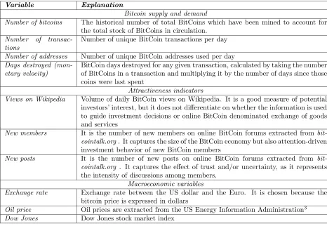
Kancs et al. (2015) employs a full multivariate VEC model as in (9), similarly to Kristoufek (2013), using daily data for the 2009-2014 period. However, differently from the latter work and in the same line of research of Bouoiyour and Selmi (2015), they considered three types of drivers to model bitCoin price dynamics: bitcoin supply and demand, bitcoin attractiveness, and global macroeconomic and financial factors. The variables used by Kancs et al. (2015) and their descriptions are presented in table 2.

Variable Explanation

Bitcoin supply and demand

Number of bitcoins The historical number of total BitCoins which have been mined to account for the total stock of BitCoins in circulation.

Number of transac-tions

Number of unique BitCoin transactions per day

Number of addresses Number of unique BitCoin addresses used per day

Days destroyed (mon-etary velocity)

BitCoin days destroyed for any given transaction, calculated by taking the number of BitCoins in a transaction and multiplying it by the number of days since those coins were last spent

Attractiveness indicators

Views on Wikipedia Volume of daily BitCoin views on Wikipedia. It is a good measure of potential investors’ interest, but it does not differentiate on whether the information is used to guide investment decisions or online BitCoin denominated exchange of goods and services

New members It is the number of new members on online BitCoin forums extracted from bit-cointalk.org. It captures the size of the BitCoin economy but also attention-driven investment behavior of new BitCoin members

New posts It is the number of new posts on online BitCoin forums extracted from bit-cointalk.org . It captures the effect of trust and/or uncertainty, as it represents the intensity of discussions among members.

Macroeconomic variables

Exchange rate Exchange rate between the US dollar and the Euro. It is chosen because the bitcoin price is expressed in dollars

Oil price Oil prices are extracted from the US Energy Information Administration3

Dow Jones Dow Jones stock market index

Table 2: Drivers of bitcoin price employed by Kancs et al. (2015).

Let consider zt=[xt, yt] be a two-dimensional time series vector with the following finite-order VAR

representation:

Θ(L)zt=εt (14)

where Θ(L) =I−Θ1L− · · · −ΘpLpis a 2×2 lag polynomial, the vector error termεtis a multivariate

white noise withE(εt) =0andE(εtε′t) =Σ, whereΣis positive definite, and deterministic terms are not

considered for ease of exposition. LetGbe the lower triangular matrix of the Cholesky decomposition

G′_G=Σ−1_{such thatE(η}

tηt) =Iandηt=Gεt. If the system (13) is assumed to be stationary, the MA

representation is given by

zt= Φ(L)εt= 

 

Φ11(L) Φ12(L)

Φ21(L) Φ22(L)       ε1t ε2t   =   

Ψ11(L) Ψ12(L)

Ψ21(L) Ψ22(L)       η1t η2t    (15)

Using this representation, the spectral density ofxt can be expressed as follows:

fx(ω) =

1 2π

|Ψ11(e−iω)|2+|Ψ12(e−iω)|2 (16)

and the measure of causality suggested by Geweke (1982) is defined as

My→x(ω) = log

2πfx(ω)

|Ψ11(e−iω)|2

= log

1 +|Ψ12(e

−iω_)|2

|Ψ11(e−iω)|2

(17)

If the measure|Ψ12(e−iω)|=0, theny does not Granger causexat frequencyω. A similar derivation

can be obtained if zt are I(1) and co-integrated, see Breitung and Candelon (2006) for more details.

Breitung and Candelon (2006) proposed a simple approach to test for the null hypothesis of non-causality (i.e. Ψ12(e−iω)|=0 using,

Ψ12(L) =−

g22_Θ 12(L)

|Θ(L)|

where g22 _{is the lower diagonal element of G}−1 _{and |Θ(L)| is the determinant of Θ(L). It follows that}

y does not causexat frequencyωif

|Θ12(e−iω)|= p X k=1

θ12,kcos(kω)− p X

k=1

θ12,ksin(kω)i = 0

where θ12,k is the (1,2)-element of Θk . It follows that a necessary and sufficient set of conditions for

p X

k=1

θ12,kcos(kω) = 0 (18)

p X

k=1

θ12,ksin(kω) = 0 (19)

Since sin(kω)=0 for ω=0 and ω=π, restriction (19) can be dropped in these cases. Breitung and Candelon (2006) proposed to test the linear restriction (18) and (19) by rewriting the VAR equation for

xtas follows:

xt=α1xt−1+...+αpxt−p+β1yt−1+...+βpyt−p+εt (20)

The null hypothesis of no granger causality at frequency ω My→x(ω)=0 is equivalent to testing the

following linear restrictions

H0:R(ω)β= 0 (21)

whereβ=[β1,...,βp]′ and

R(ω) =



 

cos(ω) cos(2ω) · · · cos(pω) sin(ω) sin(2ω) · · · sin(pω)



 

The ordinary F-statistic for (21) is asymptotically distributed as F(2,T−2p) for ω∈(0,π). Such a method can be similarly extended to cointegrated VARs by replacing xt in regression (20) with ∆xt,

whereas the right-hand side of the equation remaining the same, see Breitung and Candelon (2006, 2007) for more details. Interestingly, in the case the set of variables have a different order of integration [for examplext∼I(0) andyt∼I(1)], or simply there is uncertainty about the cointegration rank, Breitung

and Candelon (2006) suggested to follow the approach by Toda and Yamamoto (1995) and Dolado and Lu tkepohl (1996): they showed that the Wald test of restrictions involving variables which may be integrated or cointegrated of an arbitrary order, has a standard asymptotic distribution if the VAR model with optimal lag length k is augmented with a redundant number of lags dmax , where dmax is

the maximal order of integration that we suspect might occur in the our set of variables. The coefficient matrices of the lastdmaxlagged vectors in the model can be ignored and we can test linear or nonlinear

restrictions on the firstkcoefficient matrices using the standard asymptotic theory. This approach can also be used to establish standard inference for the frequency domain causality test.

example, if we add a third variable in (20) so that we get,

xt=α1xt−1+...+αpxt−p+β1yt−1+...+βpyt−p+γ1zt−1+...+γpzt−p+εt (22)

To test the null hypothesis of conditional Granger causality My→x|z(ω)=0 , we can use the usual

F-statistic to test the linear restrictions (21) on the parameter vectorβ=[β1,..., βp]′. However, Hosoya

(2001) showed that the specification in (22) may give spurious inference on causality in some cases and he suggested to use the F-statistic to test the linear restrictions (21) in the following modified regression:

xt=α1xt−1+...+αpxt−p+β1yt−1+...+βpyt−p+γ0wt+γ1wt−1+...+γpwt−p+εt (23)

wherewtare the residuals from a regression ofzt onxt,ytand the past lags of all these variables.

Bouoiyour et al. (2015) used the previous frequency-domain framework to test for unconditional [i.e. using the specification in (20)] and conditional Granger causality [i.e. using the specification in (22)] with bitcoin prices and a set of explanatory variables, to investigate the main factors influencing bitcoin price dynamics under different frequencies. First, they showed that bitcoin prices (BPI) Granger-causes the exchange-trade ratio (ETR) in the short- and the medium-run cyclical component, whereas the null hypothesis of no Granger causality from ETR to BPI is not rejected at any frequency. This last result is different from what found by Kristoufek (2015), who found a significant causality from ETR to BPI, which becomes stronger in the long term. The results by Bouoiyour et al. (2015) did not change when moving from unconditional causality to conditional causality analysis, where the employed control variables were the Chinese market index and the hash rate.

estimated output volume do not change substantially the previous evidence. These findings are quite similar to those reported by Kristoufek (2015).

In general, the analyses performed using frequency domain-based methods confirmed that the main drivers of bitcoin price dynamics are still mainly of speculative nature. However, there are several other significant factors involved, not all of them related to speculation, and the possibility to see the bitcoin technology employed for a much larger fraction of business transactions in the long term cannot be excluded.

Finally, we remark that there are also other papers which tried to model bitcoin price dynamics. How-ever, they are less comprehensive than the previous ones, the datasets are smaller and almost all of them are not peer-reviewed. We refer the interest reader to thebitcoinwikiwebpage devoted to “publications in-cluding research and analysis of Bitcoin or related areas” available athttps://en.bitcoin.it/wiki/Research

for more details.

6

Detecting Bubbles and explosive behavior in bitcoin prices

The strong volatility in bitcoin prices has sparked a strong debate whether a “substantial speculative component” (Dowd, 2014) can be an harbinger of a large financial bubble. Several statistical tests have been developed for testing the existence of financial bubbles and some of them have been recently used with bitcoin prices. These tests can be broadly grouped into two large families: tests intended to detect a single bubble, and tests intended to detect (potentially) multiple bubbles.

6.1

Testing for a single bubble

MacDonell (2014) was the first to test for the presence of a bubble in bitcoin prices using the Log Periodic Power Law (LPPL) approach proposed by Johansen et al. (2000) and Sornette (2003a,b). We describe below its main structure, while we refer the interested reader to the previous three works as well as to the recent survey by Geraskin and Fantazzini (2013) for more details.

textbook presentation of LPPLs for bubble modelling is given by Sornette (2003a), while the ex-ante diagnoses of several bubble episodes were discussed by Sornette and Zhou (2006), Sornette,Woodard, and Zhou (2009), Zhou and Sornette (2003), Zhou and Sornette (2006), Zhou and Sornette (2008) and Zhou and Sornette (2009).

The expected value of the asset log price in a upward trending bubble according to the LPPL equation is given by,

E[lnp(t)] =A+B(tc−t) +C(tc−t)·cos[ωln(tc−t)−φ] (24)

where 0< β <1 quantifies the power law acceleration of prices and should be positive to ensure a finite price at the so-called critical time tc, which is interpreted as the end of the bubble; ω represents the

frequency of the oscillations during the bubble; A > 0 is the value of [lnp(tc)] at the critical time tc,

B <0 the increase in [lnp(t)] over the time unit before the crash, C6= 0 is the proportional magnitude of the oscillations around the exponential growth, while 0 < φ < 2π is a phase parameter. It has to be noted that A, B, C and φ, are just units distributions of betas and omegas and do not carry any structural information, see Sornette and Johansen (2001), Johansen (2003), Sornette (2003a), Lin et al. (2014) and references therein.

The first condition for a bubble to take place within the JLS framework is 0 < β < 1, which guarantees that the crash hazard rate accelerates, while the second condition proposed by Bothmer and Meister (2003) is that the crash rate should be non-negative, so that

b=−Bβ− |C|pβ2_+ω2_{≥0 (25)}

Lin et al. (2014) added a third condition, requiring that the residuals from fitting equation (24) should be stationary. Lin, Ren, and Sornette (2014) used the Phillips-Perron (PP) and the Augmented Dickey-Fuller (ADF) to test for stationarity, whereas Geraskin and Fantazzini (2013) suggested to use the test by Kwiatkowski et al. (1992), given the higher power of this test when the underlying data-generating process is an AR(1) process with a coefficient close to one.

The calibration of LPPL models can be difficult due to the presence of many local minima of the cost function where the minimization algorithm can get stacked, see Fantazzini (2010), Geraskin and Fantazzini (2013) and Filimonov and Sornette (2013) for more details and for some possible solutions.

MacDonell (2014) used the LPPL model to forecast successfully the bitcoin price crash that took place on December 4, 2013, showing how LPPL models can be a valuable tool for detecting bubble behavior in digital currencies.

Cheah and Fry (2014) assumed that,

P(t) =P1(t)(1−k)j(t) where

dP1(t) = [µ(t) +σ2(t)/2]P1(t)dt+σ(t)P1(t)dWt

whereWt is a Wiener process,j(t) is a jump process

j(t) =



 

 

0 before the crash 1 after the crash

whilekrepresents the % loss in the asset value after the crash. Before a crash, we have thatP(t) =P1(t)

and using the Ito’s lemma it is possible to show thatXt= log(P(t)) satisfies

dXt=µ(t)dt+σ(t)dWt−vdj(t),

v=−ln[(1−k)]>0

(26)

Then, Fry (2014) and Cheah and Fry (2015) introduced the following two assumptions:

Assumption 1 (Intrinsic Rate of Return): the intrinsic rate of return is assumed constant and equal toµ:

E[Xt+∆−Xt|Xt] =µ∆ +o(∆) (27)

Assumption 2 (Intrinsic Level of Risk): the intrinsic level of risk is assumed constant and equal to

σ2_:

V ar[Xt+∆−Xt|Xt] =σ2∆ +o(∆) (28)

Moreover, supposing that a crash has not occurred by time t, they get

E[j(t+ ∆)−j(t)] = ∆h(t) +o(∆) (29)

V ar[j(t+ ∆)−j(t)] = ∆h(t) +o(∆) (30)

whereh(t) is the hazard rate. Using eq. (27) in assumption 1 together with eqs. (26) and (29), it follows that

which shows that the rate of return must increase in order to compensate an investor for the risk of a crash.

Fry (2014) and Cheah and Fry (2015) showed that in a bubble not only prices have to grow, but also volatility must diminish. Using eqs. (26), (28) and (30), they get

σ2(t) +v2h(t) =σ2; σ2(t) =σ2−v2h(t) (32)

The key equations (31) and (32) show that during a bubble an investor should be compensated for the crash risk by an increased rate of return with µ(t) > µ (where µ is the long-term rate of return), whereas market volatility decreases, representing market over-confidence (Fry, 2012, 2014). Moreover, it is possible to test for the presence of a speculative bubble by testing the one-sided hypothesis

H0:v= 0 H1:v >0 (33)

Fry (2014) further showed that, given the previous assumptions, the fundamental asset price when there is no bubble (v = 0) is given by :

PF(t) =E(P(t)) =P(0)eµt˜ (34)

where ˜µ=µ+σ2_{/2. Instead, during a bubble (v >0),}

Xt=N(X0+µt+vH(t), σ2t−v2H(t)), where

H(t) =Rt 0h(u)du

(35)

so that the asset value is given by

PB(t) =E(P(t)) =P(0)e ˜ µt+v−v2

2

H(t)

(36)

Equations (34) and (36), together with a proper hazard functionh(t), can then be used to compute the bubble component in the asset price, defined as the “average distance” between fundamental and bubble prices. Fry (2014) and Cheah and Fry (2015) used the following hazard function

h(t) = βt

β−1

αβ_+tβ (37)

so that the bubble component is given by,

Bubble component = 1− 1

T

T Z _P

F(t)

PB(t)

dt= 1− 1

T

T Z

1 + t

β

αβ

−v−v2 2

whereT is the sample dimension. It follows from (34) that if ˜µ <0 the fundamental asset value is zero:

lim

t→∞PF(t) = 0 (39)

Following MacDonell (2014), Fry (2015) tested for the presence of a bubble in bitcoin prices from January 1st 2013 till November 30th 2013, before the price crash of December 2013. He rejected the null hypothesis (33) and found that the parameter ˜µ is not statistically different from zero, which is compatible with a long-term fundamental value of zero. Moreover, he found that the bubble component amounts to approximately 48.7% of observed prices. These results are confirmed by several robustness checks.

6.2

Testing for multiple bubbles

The previous tests are designed to test for the presence of a single bubble and can be used to detect multiple bubbles only if repeated with a moving time window, as done by Sornette et al. (2009) Jiang et al. (2010), Geraskin and Fantazzini (2013) and Cheah and Fry (2015). Tests specifically designed for detecting multiple bubbles were recently proposed by Phillips and Yu (2011), Phillips et al. (2011) and Phillips et al. (2015) and they share the same idea of using sequential tests with rolling estimation windows. More specifically, these tests are based on sequential ADF-type regressions using time windows of different size, and they can consistently identify and date-stamp multiple bubble episodes even in small sample sizes. These tests were employed by Malhotra and Maloo (2014) to test for the presence of explosive behaviour in bitcoin prices. We will focus below on the generalized-supremum ADF test (GSADF) proposed by Phillips, et al. (2015) -PSY henceforward- which builds upon the work by Phillips and Yu (2011) and Phillips et al. (2011), because it has better statistical properties in detecting multiple bubble than the latter two tests.

This test employs an ADF regression with a rolling sample, where the starting point is given by the fraction r1 of the total number of observations, the ending point by the fraction r2, while the window

size byrw=r2−r1. The ADF regression is given by

yt=µ+ρyt−1+ p X

i=1

φirw∆yt−i+εt (40)

where µ, ρ, and φi

rw are estimated by ordinary least squares, and the null hypothesis is of a unit root

ρ = 1 versus an alternative of a mildly explosive autoregressive coefficient ρ > 1. The backward sup ADF test proposed by PSY (2015) fixes the endpoint atr2 while the window size is expanded from an

BSADFr2(r0) = sup

r1∈[0,r2−r0]

ADFr2

r1 (41)

It is important to note that the test by Phillips et al. (2011) is a special case of the BSADF test with

r1= 0, so that the sup operator becomes superfluous.

The generalized sup ADF (GSADF) test is finally calculated by repeatedly performing the BSADF test for each endpointr2∈[r0, 1]:

GSADF(r0) = sup r2∈[r0,1]

BSADF(

r2r0) (42)

The limiting distribution of (42) under the null of a random walk with asymptotically negligible drift is given by the Theorem 1 in PSY (2015), while critical values are obtained by numerical simulation. In case the null hypothesis of no bubbles is rejected, the starting and ending points of one (or more) bubble(s) can be found in a second step: the starting point is given by the date -denoted asTre- when the

sequence of BSADF test statistics crosses the critical value from below, while the ending point -denoted asTrf - when the BSADF sequence crosses the corresponding critical value from above:

ˆ

re= inf r2∈[r0,1]

r2:BSADFr2(r0)> cv

βT

r2

ˆ

rf = inf r2∈[ˆre+δlog(T)/T,1]

r2:BSADFr2(r0)< cv

βT

r2