Heat Transfer Model for Thin Solidified Material in Continuous Casting

Heat Transfer Model for Thin Solidified Material in Continuous Casting

Nobuaki Ito

Advanced Technology Research Laboratories, Nippon Steel Corporation, Futtsu 293-8511, Japan

An asymptotic explicit numerical method was developed for the Stefan problem in which a series of solidification rates and boundary temperatures for the solidified material are given and the boundary heat flux is returned. A spectral method with several basis functions of a specialized shape in the solidification problem was adopted. Combined with multi-dimensional computational fluid dynamics methods for the liquid zone, this method is adequate for resolving the thin solidified material problem for a variety of continuous casting processese.g.thin slab continuous casting, melt-spinning, twin roll casting, and edge-defined film-fed growth. The method is less expensive than conventional numerical methods and as accurate as a direct numerical approach such as the Finite Difference Method especially in the case of the Stefan number1 or in the case of variable material properties. [doi:10.2320/matertrans.MRA2007019]

(Received January 22, 2007; Accepted March 22, 2007; Published May 25, 2007)

Keywords: continuous casting, twin roll casting, Stefan problem, spectral method, basis function

1. Introduction

Heat and flow analysis in continuous casting (C.C.) around the solidification front (S.F.) provides valuable information on appropriate working conditions and morphological con-trol of casting. As shown previously, the multi-domain approach divided with discontinuous S.F. should be applied in the C.C. simulation from the viewpoint of numerical

error.1)In this approach, the entire analysis zone is divided

into a liquid and a solidified material (S.M.) zone. For the liquid zone, multi-dimensional numerical simulation is necessary for most actual process analysis because of complex geometry and variable material properties. How-ever, for S.M. analysis, a simpler approach can be applied under the following assumptions: (1) lateral heat flux is negligible. (2) solid flow is steady. (3) solid deformation is negligibly small as to the heat transfer analysis. These

assumptions are valid for a variety of types of C.C.,e.g.thin

slab casting, twin roll casting, melt spinning, and EFG. Moreover, these assumptions transform the original multi-dimensional steady conduction problem into the one-dimen-sional unsteady conduction problem with a moving

boun-dary,i.e.the Stefan problem.2–5)

As explained later, in the coupling methods between the S.M. zone and the liquid zone, weak coupling by means of a

set of given vm and feeding q00s;m back in the

solid-Stefan-problem is most appropriate. This Stefan solid-Stefan-problem could be

classified as the Inverse Stefan problem.5) _{However, this}

Stefan problem is actually a direct problem in which the problem is always well posed; therefore in the present paper, this Stefan problem is called the Thin-S.M. Problem (TSMP) to distinguish it from the ill-posed inverse Stefan problem.

Hence, the solution method for TSMP is discussed.

1.1 Analytical approach

For the multi-domain approach, the quasi-steady approach

in the S.M. is commonly used.7,8)However, the quasi-steady

approach causes a significantly large numerical error when

Stefan number Ste (¼CpðTmTs;0Þ=Lh) is not very small

(e.g. Ste>1);5) this is typical in the case of, e.g. rapid

cooling. For unsteady governing equations, analytical solu-tions exist only under simple boundary condisolu-tions as in the

Neumann problem,2) _{which is too simple a condition to}

express the actual casting processes.

1.2 Direct numerical approach

The direct numerical approach, in which the original governing equations are directly discretized into a deference equations system, could give a solution for general boundary

conditions. However, a simple and non-iterative (i.e.explicit)

solution method such as the Rung-Kutta method is not applicable to the general boundary conditions in the TSMP

for general C.C. processes, in the case of, e.g.,

time-dependent boundary temperature Ts;0, Tm. Therefore, an

iterative (i.e. implicit) direct numerical approach, e.g. the

finite difference method (FDM),9,10) _{the finite element}

method (FEM),11) _{or the boundary element method}

(BEM)12)_{is necessary for the TSMP. For this approach, a}

significantly large calculation cost is inevitable because a rather small time increment compared with the required casting time is necessary; the time increment is limited by the Courant-Friedrich-Levy (CFL) condition, which governs the calculation stability and accuracy, even in an implicit method because of the special limitation for solidification analysis. This limitation is that the movement of the S.F. in a time step must not exceed the spatial grid interval, which should be

sufficiently small for accuracy.13)Despite the recent

develop-ment of computer technology, this method remains too expensive for an iterative coupling method between the liquid and the S.M. zone; this coupling method is essential as the solution process is stabilized especially for a potentially

unstable problem such as in melt-spinning analysis.14)

1.3 Asymptotic approach

The asymptotic approach includes the classical integral

method,2) _{the perturbation method,}15–17) _{the inverse}

meth-od,18–20) _{and the spectral method.}21) _{In these methods, the} original governing equations are approximately expressed by

a sum of a series of expansion functions of x2 and t; each

expansion function could be decided analytically under the given boundary conditions.

In the perturbation method, the expansion function is

generally assumed to depend only on variable(¼hsx2)

under the assumption ofSte1;15–19)_temperature

tionTs½was expressed as then-th power ofSte. Because of

the nature of a power function, n is limited in the second

order at maximum from the view of stability of the function

shape;5)_{the shape of the final approximated function could be}

too simple to express the possible complex curve of Ts

distribution that is caused with, for example, the existence of impinging liquid flow on a specific area of the S.F. (this generally occurs in the C.C.). Moreover, the assumption

Ste1could be invalid for a rather rapid solidification.

Grzymokowski and Slota20)_{proposed an inverse method in}

which the expansion function is expressed with independent

variablesx2andtunder the given history ofhs; the method is

applicable to the wider range of the boundary conditions.

However, this method is limited in the assumption ofSte1

to decompose the expansion function. Fredrick and Greif19)

proposed the inverse method for a general magnitude ofSte.

However, in this method, the expansion function is based on

the Taylor expansion on the S.F.; the pre-defined history ofhs

is limited to a rather simple shape. In addition, in the most inverse Stefan problem, both the temperature and the heat flux on the S.F. have to be given in advance in order to

acquire the field values on the free boundary (i.e.a boundary

where no boundary conditions are given). On the contrary, the heat flux on the S.F. should be a solution variable in the TSMP; the problem to be solved is totally different regarding the inverse problem and the TSMP.

The spectral method was applied to some Stefan problems (but not to TSMP) with Fourier-expansion or

Chebyshev-polynomial approximation.22,23)These studies suggest their

applicability to the general boundary condition. However, the conventional method requires significant cost; implicit solu-tion method and/or tolerable numerical integrasolu-tions for each basis function are necessary. In the conventional method, application to the variable thermal diffusivity is generally difficult. Moreover, by definition, the problem setting in these works differs from the TSMP.

Therefore, none of the above conventional methods is appropriate for solving the TSMP in terms of accuracy or cost efficiency.

In the present paper, a non-iterative (explicit) asymptotic solution method for TSMP based on the spectral method provided with a series of specialized basis function is described. This method is applicable to the general boundary condition and variable material properties even in the case of

Ste>1.

2. Nomenclature

a: model constant

b: adjusting coefficient

Cp: specific heat

g: roll gap

h: thickness

Hr: heat resistance

Ht: heat transfer coefficient

k: heat conductivity

L: length

Lh: latent heat

m: basis function degree index

M,N: total number of basis function degree/time step

q00_{: heat flux}

qA00: steady component heat flux

Ste: Stefan number

T: temperature

Ta,dT: average/deviation component ofT

dT_{: basis function ofdT}

dTf_{: component ofdT}

t: time

t: time step

t0_:tt

i1þti=2

u: velocity

Us: pull velocity in C.C.

vA:vm

vm: solidification rate

x: coordinate value

: thermal diffusivity

1,2: model constant

": emissivity

: Boltzmann’s factor : deviation temperature

0,1,2: component of

: viscosity

: relative coordinate : density

(Subscripts)

0: C.D.-S.M. interface

fmr,lat: former/latter half of time step

in: inlet

ini: initial

l: liquid

i: time step index

j: basis function index

m: the S.F. or indexm

out: outlet

r: C.D. (roll)

ref: reference

s: S.M.

1,2: coordinate direction

B1,B2: direction along/vertical to the roll surface

(Superscripts)

o:x2 of discretized point ofdT

3. Mathematical Model

3.1 Liquid-S.M. coupling for TSMP

The strong coupling method (the field values in the liquid and the solid zone are solved simultaneously as a simulta-neous equation system) and the weak coupling method (the field values are solved individually and a coupling method is applied to the zone boundary) are candidate methods, but in this paper, the weak coupling method was adopted because strong coupling is significantly expensive.

3.1.1 Quasi-static fluid case

The TSMP could be reduced to an unsteady one-dimen-sional problem; the solution for the conventional Stefan Problem is applicable. Thus, no further discussion is required here.

3.1.2 Convective fluid in the case ofSte1

The heat transfer rate distributes on the S.F. by means of

with the liquid flow speed and the representative flow length scale that the liquid flow field is almost irrelevant to the S.M. behavior except for the heat boundary condition. Thus, the one-way coupling approach, which implies relatively small calculation cost on TSMP, from the liquid zone to the S.M. zone is applicable. The following present solution method is applicable to this case as well as the conventional method. 3.1.3 Convective fluid in the case of Ste in general

magnitude

A multi-dimensional liquid flow is affected by the S.F. distribution; thus, the two-way coupling method between the liquid and the S.M. zone is necessary. For this case, the following present solution method is appropriate because of the favorable balance of accuracy and cost; the cost is important in the iterative (implicit) solution approach between the calculation zones.

Hence, the favorable coupling boundary values in the weak coupling method are described. In zone coupling, all but one

boundary value out of four variables, i.e.Tm,vm,q00s;m, and

q00

l;m, should be given or dependent on the other boundary

values in each zone so as to make the problem well posed. The remaining variable becomes a solution variable, which must not be common between the two zones. In the boundary

variables,vm,q00

s;m, andq00l;mare dependent on each other by means of the following equation.

sLhvm¼q00s;mq00l;m ð1Þ

In sub-cooled solidification, Tm could be expressed as a

function of vm and the local material composition.24) The

solidification rate vm, which expresses the zone boundary

shape explicitly, should naturally be a solution variable for either zone. This is because the flow field, which governs the heat transfer on the S.F., is highly sensitive to the boundary shape in the multi-dimensional numerical analysis for the liquid zone. On the other hand, in the case of, for example,

Ste1 (i.e. Lh=q00

s;m!0), vm could become highly

unstable whenvmis not a solution variable but is calculated

from the other variables with eq. (1). Thus, vm should be a

solution variable. As forTm, because this variable generally

varies in a smaller range during the calculation process than

the other variables,Tmcould be acquired explicitly by means

of the function of vm as well as by means of an implicit

simultaneous solution method forvmandTm. As forq00s;mand

q00l;m, these variables exist only in the zone to which they

belong respectively;i.e.q00l;mis for the liquid zone,q00s;mis

for the S.M. zone. Thus, two sets of boundary variable

couplings are possible for the S.M. zone: (1)q00

s;mis given

from the liquid zone andvmis fed back to it. (2)vmis given

from the liquid zone and q00

s;m is fed back to it, that is the

TSMP. Although the former method is an orthodox method in

the case ofSte1,6)_{the latter was adopted in this paper for}

the following reason. In the former coupling, the iterative calculation process could become unstable because the zone interior heat is transported only diffusively in the Stefan problem. This limitation of the heat transfer route may cause

problems. For example, vm become infinite when given

q00

s;m!0, orhsbecome close to 0 (under negativevm) when

the given q00s;m is a relatively large value; this situation

commonly occurs during the calculation process. On the contrary, in the latter coupling, the iterative calculation

process is more stable because any givenvmreturns a finite

q00

s;m. In this coupling, the potential calculation instability is

transported from the S.M. zone to the liquid zone calculation. However, the calculation process in the liquid zone is

generally stable for inputq00

l;m, which is calculated from the

givenq00

s;m, because the advective heat transfer in the liquid

zone helps the problem to satisfy the given boundary

conditions; for example, any high given q00

l;m result in a

finitevmoutput, or a negativevmin a rather small magnitude

become an output for the case in which the given q00

l;m becomes zero. Therefore, the TSMP is the most appropriate for the boundary variable coupling.

3.2 Liquid model

In the TSMP,hsis so thin that the actual shape of the S.F.

could be approximated with locally variable exit velocityvA

on the imaginary flat shape S.F..25) _{This approximation}

reduces the analytical cost because exploring the S.F.-position is unnecessary. The boundary conditions on the S.F. become:

u1¼ ðs=lÞUs ð2Þ

u2¼vAðs=lÞ ¼ vmðs=lÞ ð3Þ

T¼Tm ð4Þ

As mentioned previously,q00

l;mis given andvA is a solution

variable.

3.3 S.M. model

The present solution method for the TSMP is described below.

3.3.1 Governing equation The governing equation is:

@Ts=@t¼@=@x2ðs@Ts=@x2Þ ð5Þ

Ts¼Tm; x2¼hs ð6Þ

Ts¼Ts;0; x2¼0 ð7Þ

hs¼

Zt

0

vmdt ð8Þ

Here,Tsis divided into steady componentTasand deviation

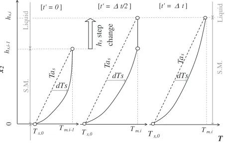
componentdTsassuming a step of change ofhs,Ts;m, andTs;0

at the middle of the time step (Fig. 1). The physical meaning of this decomposition is that the given temperature distribu-tion at the middle of the time step should become that for

steady stateTasalong the time advance when the boundary

Ts,0 Tm.i-1

T

h

s,i-1

h

s,i

x

2

[t' = 0]

hs

step

change

Ta

s

Tm.i Tm.i

Ta

s

dTs

Ta

s

[t' =∆t/2] [t' = ∆t]

Ts,0 Ts,0

S.M.

S.M.

0

Liquid

Liquid

dTs dTs

[image:3.595.316.542.73.218.2]

conditionshs,Tm, andTs;0 are kept in the rest time step;dTs correspond to the decaying component. Thus, eq. (5) becomes:

@ðTasþdTsÞ=@t¼@=@x2fs½Ts@ðTasþdTsÞ=@x2g ð9Þ

Assuming TasdTs, which is plausible for most C.C.

processes, lets½Tsbes½Tas; we can divided eq. (9) into

following the steady component and the deviation component equation.

d=dx2ðs½TasdTas=dx2Þ ¼0 ð10Þ

Tas¼Tm; x2 ¼hs ð11Þ

Tas¼Ts;0; x2¼0 ð12Þ

@dTs=@t¼@=@x2ðs½Tas@dTs=@x2Þ ð13Þ

dTs¼0; x2¼hs ð14Þ

dTs¼0; x2¼0 ð15Þ

Here, x2 represents the solidification progressing direction.

The solution of the heat flux on the S.F. in thei-th time step,

q00

s;m;i, is acquired with the sum of the heat flux for the steady

componentqA00s;m;iand the deviation componentdq00s;m;i. The

surface heat flux on the cooling deviceq00

s;0;i, is also acquired in the same way.

3.3.2 Steady component equation

The solution for eq. (10) is expressed only with the

integral of1=s. Thus, many functions forscould easily be

adopted so as to acquire an analytical solution. In the case of,

for example,sis constant,Tasbecomes:

Tas¼ ðTmTs;0Þðx2=hsÞ þTs;0 ð16Þ

In the case ofs¼a1Tasþa2 (thermal properties are often

described in this form of function in material handbooks),Tas

becomes:

Tas¼ a2þ a22þ

x2

hs

a1Tmða1Tmþ2a2Þ þ 1

x2

hs

a1Ts;0ða1Ts;0þ2a2Þ

1=2

1 a1

!

ð17Þ

The heat flux in the steady componentqA00s;m;iandqA00s;0;iis readily acquired analytically with differentiation of eq. (16) or (17)

atx2¼hs;i orx2 ¼0.

3.3.3 Deviation component equation

The collocation spectral method21)is applied to solve eq. (13); in this method, the solution is expressed by means of the sum

of a series of basis functions. The author adopted the following basis functiondTi;j(irepresents thei-th time step,jrepresents

the j-th basis function). In time stepi, the basis functions are initialized at the middle of the time step just after the

above-mentioned step change ofhs andTs. The initial value of the basis function is:

dTi;j;ini¼ ðdToi;j=x2oi;jÞx2 ¼1i;jx2;

0x2x2oi;j ð18Þ

dTi;j;ini¼ fdToi;j=ðhs;ix2oi;jÞg ðhs;ix2Þ

¼2i;jðhs;ix2Þ; x2oi;j<lx2hs;i ð19Þ

The initial basis function is Fourier expanded; them-th expanded term for thej-th basis function,dT f

i;j;m;iniis:

dT fi;j;m;ini¼

2

hs;i

Zi;jhs;i

0

1;i;jx2sin

mx2

hs;i

dx2

þ

Zhs;i

i;jhs;i

2;i;jðhs;ix2Þsin

mx2

hs;i

dx2

sin mx2 hs;i

ð20Þ

¼ 2dT

o i;j

ðmÞ2i;jð1i;jÞ

sin½i;jmsin

mx2

hs;i

Here,i;j¼x2oi;j=hs. The temperature distributiondT fi;j;m;ini always satisfies eq. (14) and (15); therefore, the solution of

eq. (13) for the original initial condition could be expressed with the sum of the solution of eq. (13),dT f

i;j;m, for each initial

conditiondT f

i;j;m;ini. Under constants;i;jfor eachdT fi;j;m, the solution of eq. (13)dT fi;j;mbecomes as follows in the period

of0t0_t

i=2,t0¼tti1þti=2.

dT fi;j;m¼

2dToi;j

ðmÞ2i;jð1i;jÞ

sin½i;jmsin

mx2

hs;i

exp m hs;i

2

s;i;jt0

" #

ð21Þ

The partial differentiation ofdT f

i;j;manalytically becomes:

@dT f i;j;m

@x2

¼ 2dT

o i;j

ðmÞ2i;jð1i;jÞ

sin½i;jmcos

mx2

hs;i

exp m hs;i

2

s;i;jt0

" #

ð22Þ

In the spectral method, the deviation heat flux on the S.F. for the latter half of thei-th time step (ti1þti=2tti),dq00s;i;lat,

is approximated with the sum of the basis function dTi;j differentiation, which is expressed with the sum of dT fi;j;m

dq00s;i;lat¼

2

ti

XN

j¼1

XM

m¼1

bi;j

Zti=2

0

@T f i;j;m

@x2

dt0

¼X

N

j¼1

XM

m¼1

bi;j

4hs;idToi;j

ðmÞ3s;i;ji;jð1i;jÞti

sin½i;jmcos½m ð23Þ

1exp m

hs;i

2

s;i;j

ti

2

" #

( )!

bi;j¼

@Tas

@x2

_x2¼hs;i

hs;ix2oi;j

Tm;iT2oi;j

ð24Þ

Here,bi;j is an adjusting coefficient against the numerical error caused by regarding the temperature gradient at the S.F. as

linear.

In the former half of the (iþ1)-th time step, no boundary condition changes from the latter half of thei-th time step.

Identical basis functions to those for thei-th latter time step could be adopted to acquire the heat flux. Therefore, the deviation

heat flux on the S.F. for the former half of thei-th time step (ti1<t<ti1þti=2),dq00s;i;fmr, could be expressed with the

basis functions in the (i1)-th time step:

dq00s;i;fmr ¼

XN

j¼1

XM

m¼1

bi;j

4hs;i1dToi1;j

ðmÞ3

s;i1;ji1;jð1i1;jÞðti1þtiÞ

sin½i1;jmcos½m 1exp

m hs;i1

2

s;i1;j

ðti1þtiÞ

2

" #

( )! ð25Þ

Consequently, the deviation heat flux for time step i dq00

s;i becomes:

dq00s;i¼ ðdq00s;i;fmrþdq00s;i;latÞ=2 ð26Þ

The total number of basis functionsNcould change between

the former and the latter time step; in this case, dTo

i;j is

interpolated with newx2oi;j.

The distance between the S.F. and the x2oi;j next to the

S.F.,x2oi;N, should be set no more thanhs;i(¼vmti) to

express the above step change of hs accurately. This

condition limits the minimum number ofM required:

M¼ ðhs;i=hs;iÞ=ð2Þ ð27Þ

Whenhs;iis significantly small,Mcould be a huge value.

However, in this condition, the step change of hs in a time

step is so small that it hardly affects the temperature field; the

calculation could be performed so that no change ofhsoccurs

during the time step. Therefore, the basis function of the last

time step could be carried over; no limitation emerges forM.

Thus,M could be always a finite value.

The thermal diffusivity for thej-th basis function in thei-th

time,s;i;j, could be set:

s;i;j½T ¼s½Taðx2oi;jÞ ð28Þ

Equation (28) generally causes a numerical error. However, because of its function shape, the deviation temperature at

x2oi;j,dTi½x2oi;j, tends to be most affected by its component

dT

i;j½x2oi;j, which gives a plausible s at x2oi;j. Thus, the

numerical error was relatively small as described in the following chapter.

To decompose the initial deviation temperature

dTi½x2;t0¼0 into the N initial basis functions dTi;j;ini,

Nsimultaneous linear equations should be solved so that the

sum of dTi;j;ini½x2oi;j (j¼1;N) agrees with the given

dTi½x2oi;j;t0¼0, which is the collocation method.21) The

inverse matrix for solving the simultaneous equations only

depends on i;j.; the given dTi½x2oi;j;t0¼0fixes the basis

functions.

3.4 Cooling device (C.D.) model

The C.D.-Model is modeled after the heat transfer at the surface (the other side of the liquid side) of S.M. by means of giving the surface temperature. The C.D.-Model could be divided into two cases with the magnitude of the Biot number

Bi (¼Hths=ks or hs=ðHrksÞ); that is the

Surface-Heat-Resistance Dominating Case (Bi<1) and the

Interior-Heat-Resistance Dominating Case (Bi>1).

3.4.1 Surface-heat-resistance dominating case

This is typical in the case of an open casting of ribbon such as EFG. The surfaces of a ribbon are cooled relative weakly with the radiation and the heat advection by atmosphere. The

inner heat resistanceh=ks is relatively small. Thus, the heat

resistance at the surfaces is dominant in total heat transfer. Consequently, the initial surface temperature in casting is close to the melting point. The surface temperature gradually reduces in a wide range to the atmospheric temperature during casting.

The boundary condition at the surface is:

ksð@Ts;0=@x2Þ ¼HtðTs;0TaÞ þ" ðTs;04Ta4Þ ð29Þ

In this boundary condition, surface temperatureTs;0is defined

only implicitly. Therefore,Ts;0should be decided iteratively.

3.4.2 Interior-heat-resistance dominating case

This is typical in the case of the other rather ordinary C.C.

processes, where C.D. (e.g.a mold, a cooling roll) is usually

designed to be composed with highly heat conductive materials for efficient cooling. Most of these C.D. are also accompanied by massive water cooling on their back. To discuss the interior heat resistance, supposing a steady heat transfer for the Stefan problem, the heat flux through the S.M.

q00s¼ ðTmTr;0Þ=ðHrþh=ksÞ ð30Þ

q00s¼ ðTs;0Tr;0Þ=Hr ð31Þ

In most C.C. processes, the heat resistance at the surfaceHris

designed to be smaller than inner heat resistancehs=ksexcept

for at very early solidification (i.e. at very small hs).

Therefore, in most areas, the interior heat resistance is dominant in the total heat transfer.

Because the actual processes correspond to the unsteady Stefan problem, the actual temperature distribution in the S.M. has to be calculated not with eq. (30) but with the S.M.-Model. However, eq. (31) could be valid in the actual processes because the thickness of the heat resistance layer at the C.D. surface is so thin that the local quasi-steady state is expected there.

When the contact between S.M. and C.D. is perfect (i.e.

Hr¼0) and the surface temperature of the C.D. is regarded

as constant valueTr;0, the surface temperature of S.M.Ts;0is

equal to Tr;0. Otherwise, Ts;0 should be decided iteratively

with the combination of eq. (31), the S.M.-Model, and the

C.D. Model (i.e. Implicit-Coupling method) in general.

However, the following plausible assumptions in the C.C. could allow escape from the expensive Implicit-Coupling method to a simple Explicit-Coupling method. The

assump-tions are: (1) Tr;0Tr;ref TmTs;0 (2) ð@Ts;0=@tÞt

TmTs;0. The calculation steps of the Explicit-Coupling

method are: (1) At a certain time step i, the surface

temperature of the C.D. Tr;0 is calculated with the

C.D.-Model, which is explained later. The value of the surface heat

flux of the S.M. at the previous time stepq00s;0;i1 is used as

the heat boundary condition at the C.D. surface. (2) The

surface temperature of the S.M. at time step i Ts;0;i is

calculated with eq. (31) on the condition of q00

s¼q00s;0;i1. (3) The temperature distribution in the S.M. is calculated

with the S.M.-Model. This temperature distribution givesq00

s for the next time step calculation.

The C.D.-Model gives the instantaneous surface temper-ature of the C.D. from the given history of the surface heat flux by way of solving the temperature distribution in the C.D.. In the relevant calculation area, the heat transfer analysis reduces to a boundary value problem for heat conduction in a fixed calculation area. Thus, there are analytical solutions for typical analysis cases. Here, for example, the solution for melt spinning is described.

The material properties of C.D. are set constant because of its relatively less changeable temperature. The C.D. is regarded as a semi-infinite material and the initial temper-ature is uniform. As the actual melt spinning process condition, these assumptions are plausible. The governing equation is as follows.

@r=@t¼ rð@2r=@x22Þ ð32Þ

r¼TrTr;ini ð33Þ

Because of the equation linearity, the temperature

distribu-tion at time stepicould be composed with superposition of

the response deviation-temperature distributions to the rectangular-heat-input at every past time step. Each response deviation-temperature distribution is calculated with a super-position of the response deviation-temperature distributions to two step-heat-input whose beginning time differs. For a

semi-infinite body, the deviation-temperature distribution

of response to a step-heat-input that begins at time tj, 1j,

under the conditions of1j;ini¼0,1jjx2!1¼0,q00r;0 ¼0

(t<tj), andq00r;0¼q00r;0;j(ttj) is as follows.3)

1j½t ¼q00r;0;j0½ttj

0½t ¼ 1 kr

( 2

ffiffiffiffiffiffiffi rt

r

exp x2

2 ffiffiffiffiffiffirt

p

2

" #

x2erfc

x2

2 ffiffiffiffiffiffirt

p

)

ð34Þ

The deviation-temperature distribution of the response to a

rectangular-heat-input, 2j, under conditions of q00r;0 ¼0

(t<tj,t>tjþ1) andq00r;0¼q00r;0;j(tjþ1ttj) is:

2j¼q00r;0;jð0j½ttj 0j½ttjtjÞ ð35Þ

Thus, when each time step is constant (i.e. ti¼t), the

deviation-temperature distribution at time ti (¼it)

be-comes:

r;i¼

Xi

j¼1

2j½titj

¼X

i

j¼1

q00r;0;j0½ðijþ1Þt

X

i1

j¼1

q00r;0;j0½ðijÞt ð36Þ

¼q00r;0;10½it þ

Xi1

j¼1

ðq00r;0;jþ1q00r;0;jÞ0½ðijÞt

Surface temperature Tr;0 is defined at x2¼0 in eq. (36).

Consequently,Tr;0 becomes:

Tr;0 ¼

2

kr

ffiffiffiffiffiffiffiffiffiffiffi rt

r

q00r;0;1

ffiffi i p

þX

i1

j¼1

ðq00r;0;jþ1q00r;0;jÞ

ffiffiffiffiffiffiffiffiffi ij p

( )

þTr;ini

ð37Þ

3.5 Advantage of the present solution method

The present method gives the solution temperature field explicitly without the limitation of time increment. In addition, this method requires less computer memory because of the nature of the one–dimensional method and less limitation for the spatial interval; the limitation occurs only on the S.F.

The present model analytically gives the temperature differentiation, with which the heat flux is expressed, at any

point ofx2. On the contrary, in the finite difference methods,

the differentiation is only acquired with the difference approximation; thus, a micro spatial interval is necessary to achieve accuracy. The present method is also applicable

to the Stefan problem in Ste1; most of the analytical

methods and the perturbation method are incapable of handling this condition. Moreover, the present model

considers general boundary conditions and s variation by

different material properties); on the contrary, the

conven-tional explicit spectral method is weak at the s variation

because of its approximation by means of only a single series of the decomposed functions (each decomposed function corresponds to the basis function). These advantages are due to the shape of the present basis function for the spectral method.

Therefore, the present method is advantageous in the balance of cost and accuracy.

4. Validation

4.1 Schwarz-like problem

A simple and typical Stefan problem, which is similar to

the well-known Schwarz Problem,2) _{was solved compared}

with the conventional method. 4.1.1 Problem description

The one-dimensional unsteady heat conduction problem between a roll and melt (liquid and S.M.) was solved under

the three conditions of Table 1 (x2direction. The origin is the

interface between the melt and the C.D.). These conditions correspond to actual casting processes as ferroalloy casting

with a copper C.D., in whichStecould become the largest.

The intention of the validations for these cases is as follows;

(1) CASE 1: the applicability to the infinite largeSte(Lh¼0

means an amorphous casting). (2) CASE 2: the applicability to the highly variable heat conductivity. (3) CASE 3: the

applicability to the largeHrandLh. As the initial condition,

the temperature for both the melt and the C.D. are set individual reference temperatures. The boundary conditions

atx2;r;ref andx2;s;ref are insulation. Five basis functions with

100-degrees were adopted for eachdT. The time steptis

2 106_{s; under this value oft, the time integral ofq}00

m

proved to be constant fort.

The simulation for the same problems was performed according to a conventional method; That is the finite volume

method (FVM),25)which is the most popular computational

fluid dynamics model for engineering purposes. The FVM

was accompanied by the enthalpy method13) for the

solid-ification model. The mesh number 4000 and the time

increment5 108_{s were adopted so as to make the integral}

of q00

m independent from the discretizing parameters. The

liquidus temperature was set 2 K above the solidus

temper-ature (Tm) for calculation stability. The calculated Tm

position-transition was applied to the present method as the

pre-definedhs.

4.1.2 Results and discussion

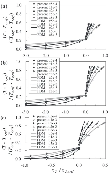
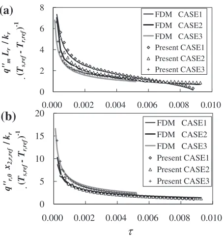
The present temperature distributions agree with the conventional method within 5% (as a local value) for all cases (Fig. 2). The agreement for the heat fluxes is within 10% (as a local value) and 2% (as a time integral value) (Fig. 3). These accuracies are sufficient for ordinary engi-neering purposes. As for calculation time, the conventional

method took 8 min for the casting term of 104_{s, whereas}

only about 1 second is necessary for the present method; in

both calculations, an IntelXeon3 GHz CPU26)_{was used.}

Therefore, the present method is accurate and cost effective

even in the case ofSte1or variable material properties.

4.2 Twin roll casting

A more practical problem was solved compared with the experimental data in the twin roll casting of paraffin

performed by Shiomi & Osakada.27)

4.2.1 Problem description

The geometry and material properties follow those of the

(a)

0.0 0.2 0.4 0.6 0.8 1.0

-3.0 -2.0 -1.0 0.0 1.0

(

T

-

Tr,ref

)

/ (

Ts,ref

-

Tr,ref

)

present t:5e-4 present t:1e-3 present t:2e-3 present t:5e-3 present t:8e-3 FDM t:5e-4 FDM t:1e-3 FDM t:2e-3 FDM t:5e-3 FDM t:8e-3

(b)

0.0 0.2 0.4 0.6 0.8 1.0

-3.0 -2.0 -1.0 0.0 1.0

(

T

-

Tr,ref

)

/ (

Ts,ref

-

Tr,ref

)

present t:5e-4 present t:1e-3 present t:2e-3 present t:5e-3 present t:8e-3 FDM t:5e-4 FDM t:1e-3 FDM t:2e-3 FDM t:5e-3 FDM t:8e-3

(c)

0.0 0.2 0.4 0.6 0.8 1.0

-1.0 -0.5 0.0 0.5

x2 / x2,s,ref

(

T

-

Tr,ref

)

/ (

Ts,ref

-

Tr,ref

)

present t:5e-4 present t:1e-3 present t:2e-3 present t:5e-3 present t:8e-3 FDM t:5e-4 FDM t:1e-3 FDM t:2e-3 FDM t:5e-3 FDM t:8e-3

[image:7.595.312.542.71.437.2]

Fig. 2 Temperature Distribution in the x2 direction. (a) CASE 1, (b) CASE 2, (3) CASE 3.

Table 1 Calculation conditions.

CASE 1 CASE 2 CASE 3

Tr;ref /K 300

Ts;ref /K 1573

Tm /K 1023 1423

x2;r;ref /mm 10000

x2;s;ref /mm 30 100

kr /W/mK1 400 150

ks /W/mK1 25 0:019 Tsþ0:1 30

r /kg/m3 ₈₇₀₀

s /kg/m3 ₆₇₀₀

Cpr /J/kgK1 400

Cps /J/kgK1 700 450

Lh /J/kg 0 2:3 105 ₀

Hr /mK/W 0 1:0 107

[image:7.595.49.290.82.293.2]

experiment.27)_{The cooling roll rotates at peripheral speedu} r 0.012 m/s in the outlet direction. To accommodate the problem to the present method, the entire calculation zone is divided into the liquid and S.M. zone at the S.F. (solidus

temperature Tm) (Fig. 4). The following assumptions are

imposed; (1) the curvatures of the roll and the S.F. are ignored in the S.M. zone. (2) the curvature variation of the S.F. is ignored in the liquid zone. (3) the solidification is expressed with the outflow at the S.F. in the liquid zone as in Ref. 24). (4) no deformation in the S.M. occurs. (5) the heat transfer in the S.M. is regarded as the Stefan problem. The

coordinate system along (the xB1 direction) or vertical (the

xB2direction) to the S.F. is set. The boundary conditions are:

(1) Liquid zone

(inlet) u1;in¼giniur=Lin, (gini¼5 104m), u2;in¼0

T ¼Tin

(the S.F.)uB1¼ur,uB2¼vAs=l,T¼Tm

(outlet) Free outlet (2) S.M. zone

(roll surface)Tr¼288K,Hr¼2 103mK/W

(the S.F.)T¼Tm,hs¼

R vAdt

In the liquid zone, the flow and temperature field was

solved with FVM;25)_q00

s;mis given and returnshs(i.e.vA) to

the S.M. zone so that (q00l;msLhvA) agree withq00s;m by

means of adjusting thevAdistribution. Moreover,Linand gap

g is adjusted during the iteration process with mesh

deforming technique28)_{so as to satisfy the condition of the}

outlet velocity u1;out¼ur. In the S.M., the given steady hs

alongxB1is translated into transienthsin the Stefan problem;

and q00

s;m is returned to the liquid zone (i.e. TSMP). The

TSMP is solved with the present method. The iterative calculation between the liquid zone and the S.M. zone is

performed until bothhsandqs;mdoes not change by iteration.

4.2.2 Results and discussion

Despite the rather simple geometry, the calculated velocity field (Fig. 5) and the shape of the S.F. curve (Fig. 6) are complicated because of the existence of a recirculation flow in the liquid zone. The recirculation flow transfers the cooled mush from around the outlet to the inlet direction; this phenomenon was clearly observed in some experimental

cases.27) _h

s is rapidly increased around the outlet; this is

because the liquid is so thin (xB2 direction) there that the

temperature of the main stream more rapidly decreases in the

stream (xB1) direction than in the upper-stream. Therefore,

the simplification derived from the assumption of, for example, the static flow field or a classical boundary layer theory (these assumptions were common in the conventional Stefan problem approaches) is inadequate.

The difference ofhsat the outlet between the experimental

and the present result is 7%. The present method seems to express an actual casting process as well as the conventional full-2-dimensional FEM described in Ref. 28), in which the

given material properties were adjusted so that thehsresult

with FEM analysis agree with the experimental data. : u / uB1 = 1.0

the S.F.

Fig. 5 Velocity vector distribution in the liquid zone.

0.0 0.2 0.4 0.6 0.8 1.0

0.0 0.2 0.4 0.6 0.8 1.0

2 x

B1

/ D

r

h

s

/

g

ini

Present

Experimental27)

Fig. 6 The S.F. distribution. the S.F.

Symmetry

Inlet

Outlet 0.045m

φ

0.1m

Gap :

g

0 x1

x2

0

x_B1 xB2

(Cooling Roll)

Lin

Fig. 4 Schematic of the system.

(a)

0 2 4 6 8

0.000 0.002 0.004 0.006 0.008 0.010

q"

m

Lr / k

r

.

(

Ts,ref

- T

r,ref

)

-1

FDM CASE1 FDM CASE2 FDM CASE3 Present CASE1 Present CASE2 Present CASE3

(b)

0 5 10 15 20

0.000 0.002 0.004 0.006 0.008 0.010

q"

r,0

x

2,r,ref

/

kr

.

(

Ts,ref

- T

r,ref

)

-1

FDM CASE1 FDM CASE2 FDM CASE3 Present CASE1 Present CASE2 Present CASE3

τ

[image:8.595.56.284.71.312.2] [image:8.595.312.540.77.202.2] [image:8.595.316.541.238.379.2] [image:8.595.57.284.358.471.2]

However, the uncertainty analysis regarding neither the experimental data nor the material properties is described in Ref. 28). Thus, the quantitative accuracy estimation is not to be discussed for this case until at least accurate material properties for the experiment are provided.

5. Conclusion

A spectral method in which basis functions are specialized in the solidification problem was developed for the Stefan problem. In combination with the multi-dimensional CFD methods for the liquid zone, this method is adequate for the thin solidified material problem for a variety of continuous casting processes. The method is as accurate as conventional direct numerical methods but less expensive, especially in the

case ofSte1or the variable material properties condition.

REFERENCES

1) N. Ito: J. Thermal Sci. and Technology2(2006) 54–65.

2) H. S. Carslaw and J. C. Jaeger:Conduction of Heat in Solids 2nd Edition, (Oxford university Press, Oxford, 1959) pp. 282–296. 3) B. Gebhart:Heat Conduction and Mass Diffusion, (Mcgraw-Hill, USA,

1993) pp. 173–273.

4) S. C. Gupta: The Classical Stefan Problem, (Elsevier, Amsterdam, 2003) pp. 85–270.

5) L. S. Yao and J. Prusa: Adv. Heat Transfer19(1989) 1–95. 6) P. H. Steen: Annu. Rev. fluid Mechanics29(1997) 373–397. 7) M. S. Sadeghipour, M. N. O¨ zisik and J. C. Mulligan: Trans. ASME J.

Heat Transfer104(1982) 316–322.

8) C. K. Hsieh: Int. J. Heat Mass Transfer38(1995) 71–79.

9) S. Toda, H. Sugiyama, H. Owada, M. Kurokawa and Y. Hori: Proc. Int.

Heat Transfer Conf. 8th, San Francisco (1986) 1745–1750.

10) A. K. Verma, S. Chandra and B. K. Dhindraw: Appl. Math. Comput.

158(2004) 573–584.

11) N. C. W. Kuijpers, F. J. Vermolen, K. Vuik and S. van der Zwaag: Mater. Trans.44(2003) 1448–1456.

12) P. C. Hong, T. Umeda and Y. Kimura: J. Japan Inst. Metals48(1984) 1099–1105.

13) I. Ohnaka: Computer Heat Transfer Solidification Analysis (in Japanese), (Maruzen, Tokyo, 1985) pp. 176–208.

14) D. Ishihara, S. Yoshimura and G. Yagawa: Trans. JSME B68(2002) 2451–2459.

15) R. I. Pedroso and G. A. Domoto: Int. J. Heat Mass Transfer16(1973) 1816–1819.

16) D. Lecomte and J.-C. Batsale: Int. J. Heat Mass Transfer34(1991) 894–897.

17) J. Caldwell and Y. Y. Kwan: Int. J. Heat Mass Transfer46(2003) 1497–1501.

18) N. Zabaras and K. Yuan: Numer. Heat Transfer B26(1994) 97–104. 19) D. Frederick and R. Greif: Trans. ASME J. Heat Transfer107(1985)

520–526.

20) R. Grzymokowski and D. Slota: Int. J. Comput. Math. With Appl.51

(2006) 33–40.

21) A. Kuroda:Analysis of Turbulent Flow, (Univ. of Tokyo Press, Tokyo, 1995) pp. 119–136.

22) R. Spall: Int. J. Heat Mass Transfer38(1995) 2743–2748.

23) Z. Dursunkaya and S. Nair: Trans. ASME J. Appl. Mech70(2003) 633–637.

24) J. K. Carpenter and P. H. Steen: Int. J. Heat Mass Transfer40(1997) 1993–2007.

25) S. R. Mathur and J. Y. Murthy: Numer. Heat Transfer B31(1997) 195– 215.

26) Intel and Xeon are registered trademarks of Intel Corporation. 27) M. Shiomi, K. Mori and K. Osakada: Trans. JSME C61(1995) 3728–

3733.