A Two-Dimensional Conjugate Heat Transfer Model for Forced Air Cooling of an Electronic Device

A. Zebib Department of Mechanical and Aerospace Engineering, Rutgers University, New Brunswick, NJ 08903 Y. K. Wo AT&T Bell Laboratories, Holmdel, NJ 07733

A Two-Dimensional Conjugate Heat

Transfer Model for Forced Air

Cooling of an Electronic Device

Thermal analysis of forced air cooling of an electronic component is modeled as a two-dimensional conjugate heat transfer problem. The velocity field in a constricted channel is first computed. Then, for a typical electronic module, the energy equation is solved with allowance for discontinuities in the thermal conductivity. Variation of the maximum temperature with the average air velocity is presented. The importance of our approach in evaluating possible benefits due to changes in component design and the limitations of the two-dimensional model are discussed.

Introduction

The current trend for miniaturization in semiconductor devices is posing challenging problems for the heat transfer analyst. Reliability considerations require knowledge of the highest temperature as well as the thermal stress distribution within the device. Typical power-density dissipation in modern electronic systems can reach 2 Watts in a volume of about 3 X 10"8 m3. The primary mechanism exploited for heat

removal is forced air cooling.

The state of the art in thermal design of electronic equip-ment involves solving the heat conduction problem in the in-dividual packages. Quick methods of design may be found in specialized books such as the one by Steinberg [1]. More ac-curate computations of the conduction problem are routinely performed and are considered of proprietary nature by the manufacturers of the components. These approaches, however, rely completely on an assumed average convective heat transfer coefficients and on an assumed known local air temperature. The recent paper by Hannenman [2] discusses these issues. Heat transfer coefficients and a superposition technique for isothermal arrays of cubic blocks were deter-mined by Arvisu & Moffat [3]. Experiments to determine the convective heat transfer coefficients were performed by Spar-row, Niethammer and Chaboki [4],

In this paper we consider the conjugate heat transfer prob-lem which models forced convection air cooling of a single module. Figure 1 shows a possible module configuration. The silicon chip is embedded in a ceramic chip-carrier and is sur-rounded by an air gap on the lower side. The module is mounted on a printed circuit board whose structure is shown in Fig. 2. The duct flow assembly is sketched in Fig. 3. All the relevant dimensions are indicated in Figs. 1-3. The heat generated in the chip is conducted though the air gap and the ceramic chip-carrier. The major part of this heat is convected to the cooling air, while the rest is conducted into the circuit board and then convected to the surroundings. All of these

Contributed by the Heat Transfer Division for publication in the JOURNAL OF ELECTRONIC PACKAGING. Manuscript received at ASME Headquarters October 21, 1988.

CERAMIC

U — d x a — » - | I [ S I L I C O N ] dya

AIR | T d x g e-i

-

dxs-dys

t

dza dzs

t

1

Fig. 1 Side and bottom views of a typical electronic component. The heat is dissipated in the silicon chip which is located at the center of the ceramic carrier and is surrounded by an air gap.

dye COPPER

td EPOXY GLASS

dye COPPER

Fig. 2 Printed circuit board. The epoxy glass layer is sandwiched be-tween a pair of thin copper layers.

features including the different thermal conductivities, as well as the variation of the local convective coefficients and cooling air temperature are all accounted for in the conjugate modeling.

Although the true flow field is three-dimensional, we assume a two-dimensional flow. Heat flow from the lower sur-face is assumed due to free convection with a constant heat

Journal of Electronic Packaging MARCH 1989, Vol. 111/41

Copyright © 1989 by ASME

1 y AIR FLOW X >

-j.

1

Fig. 3 Duct flow assembly. This Is the computational domain for the temperature field. Also shown is the coordinate system.

transfer coefficient. The top surface of the duct is taken as in-sulated. Further, we assume laminar flow conditions to prevail. Thus the temperature rise predicted by the model is expected to be conservative.

Mathematical Model

If we assume constant thermodynamic properties, the velocity and pressure fields are uncoupled from energy con-siderations. In the usual two-dimensional Cartesian notations, the Navier-Stokes equations are

V - V = 0,

( p V V ) V = - yp+ V ( / J W ) .

The boundary conditions are

V(CV) = ( 6 U ( £ ) ( 1

axv(oo,_v)=o,

V(x,0) = 0,

Y(x,yl) = 0.

Where U is the average air flow velocity and we have as-sumed a fully developed velocity profile at the entrance which is located sufficiently far from the module. Likewise, the outflow boundary condition is imposed far downstream from the module. It should be noted that no boundary conditions are imposed on the pressure, which is determined uniquely, up to an additive constant, through consideration of the continui-ty equation (la).

Finite-volume solutions of (1-2) are computed on a stag-gered grid. The details of the numerical scheme and the itera-tion procedure we use to solve the discretized equaitera-tions are described in detail by Patankar [5]. Briefly, the computational region is divided into rectangular control volumes with the grid points located at the geometric centers of these cells. Ad-ditional boundary points are included where the boundary conditions (2) are imposed. We include the region occupied by the module in the computation. This is accomplished by

set-_ N o m e n c l a t u r e

= specific heat of air at con-stant pressure (la) (lb) (,2a) (2b) (2c) (2d) in o o o o

L

~|-0 . ~|-0 0 . 0 5 0 . 1 0 0 . 1 5 0 . 2 0 0 . 2 5 0 . 3 0

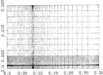
Fig. 4 Computational mesh for the velocity field. There are 50 and 35 control volumes in the x and y directions, respectively. The highest den-sity of mesh point is at the chip site where a total of 63 control volumes are allocated. Note that the computational region extends only to x = 0.264 m.

ting the viscosity in this region very large and making use of the harmonic mean for the viscosity [5] (as well as for the ther-mal conductivity when we solve the energy equation) at sur-faces of discontinuity which we choose to coincide with the control surfaces. The discretized equations are obtained by in-tegrating equations (1) over the control volumes with assumed local linear variations in any of the primitive variables. The convection and diffusion fluxes are approximated by a power-law scheme. A line-by-line iteration to solve the discretized equations is used with one iteration comprising four double sweeps of the field. Under-relaxation in solving for u and v was required; a relaxation factor of 0.75 was used throughout. With the velocity field at hand, we now consider the temperature field. The energy equation is

(pcp\.V)T=v(KvT)+q. (3)

where T is the temperature rise above surroundings. The boundary conditions are

T(0,y)=0, dxT(oo,y) = Q,

[KdyT=hT]y=_td

dyT(x,yl) = 0.

(4a) (4b) (4c) (4d)

Here h is the free convection coefficient of heat transfer from the board to surroundings. Finite volume solutions to (3-4) are obtained in a similar manner. In our two-dimensional model, we assume uniformity over a depth of ex-tent dza (Fig. 1). Thus the heat generation per unit volume

q = W/(dxa x dya x dza), where Wis the power dissipation. It

dxa, dxg, dxs, dya, dye, yi, dza, dzs, td, xlft, xrit,

= physical dimensions of

duct, module and circuit board assembly, Figs. 1-3

T, h, K, P, q,

r,

m a x '

U,

= free convection heat

transfer coefficient = thermal conductivity = pressure

= volumetric rate of heat generation

= temperature above surroundings

= highest temperature rise = velocity component in the

x direction at x=0

u,

w,

= average air velocity in the x direction

= velocity vector

= velocity component in the

y direction

= Cartesian coordinate = Cartesian coordinate = power dissipation = dynamic viscosity = density

J_ J_

0.05 0.10 0.-15

Fig. 5(b)

0.20

0.05 0.10

0.0122 —0.011 —0.01

-0.007

-0.005 -0.004 -0.003 -0.002

0.0005

0 0.05 0.10 0.15 0.20 0.25 0.30 Fig. 5(a)

0.25 0.30

0.15 0.20 0.25 0.30 Fig. 5(c)

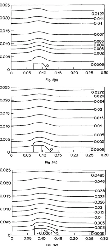
Fig. 5 Streamlines corresponding to different flow velocities, (a)

U = 0.5 m/s, (b) U = 1.1 m/s, (c) U = 2 m/s. The numbers on the streamlines

are the values of the volumetric streamfunction. There is now flow rever-sal ahead of the module at these velocities.

should be noted here that the volumetric heat generation is zero everywhere, except in the chip where its value is q. Due to the large number of parameters which influence the temperature level in the chip, we will hold all of the physical dimensions constant at the values given in Table 1. In Table 2 we list the relevant thermal properties used in the computa-tions. From equations (3-4) it is then evident that we must consider the variation of T as a function of U, h, and q. However, due to the linear dependence of T on q, only one value of W is considered from which one obtains the temperature rise per Watt of heat dissipation.

0.8 1.0 1.2 1.4 1.6 AIR VELOCITY m/s

1.8 2.0

Fig. 6 Variation of Tmax with U. The higher temperatures correspond to h = 2 W/m2C, while the lower curve is for h = 3 W/m2C. The power

dissipation is fixed at 1 Watt.

Table 1 Physical dimensions (m)

xlft dxs xrit dxa dxg dye td dys dya yi dza dzs

0.072 0.024 0.168 0.0065 0.015 0.0000375 0.0016 0.0025 0.00055 0.025 0.0065 0.05

Table 2 Thermal property

Material Air Ceramic Copper Epoxy-glass Silicon

p = 1 . 1 6 k g / m3 cp = 1007 j / k g C H = 0.000018 N.s/m2 Thermal conductivit;

W/m.C 0.0263 35.0 390.0 0.290 100.0 Results and Discussion

The solution for the flow field was performed on the nonuniform mesh shown in Fig. 4. The computational region is covered by 50 and 35 control volumes in the x and y direc-tions, respectively. The highest density of control volumes is at the chip location where all the heat is generated. Computa-tions obtained on a finer mesh showed virtually no changes in the flow field. Starting with a fully developed velocity field (with V = 0 in the module), it took about 250 iterations to con-verge. Convergence was declared when the maximum change in u and v per iteration cycle was less than 10 ~4 xU.

Because air velocities (U) in the range 0.52 m/s are used in practice [3], we compute the flow field for three values cover-ing this range. The streamlines are shown in Fig. 5. As [/in-creases the length of the separated region downstream from the module increases accompanied by an increased strength of the reversed flow. At these values of U there was no indication in the computed solutions of the occurrence of Moffatt [6] corner eddies ahead of the module. Similar computations were performed by Patankar [7], however he did not report the values of the flow parameters and thus no comparison be-tween his and our results is possible.

Journal of Electronic Packaging MARCH 1989, Vol. 111/43

0.05 0.-10 0.-15 0.20 0.25 0.30 Fig. 7(a)

0.10 0.15 Fig. 7(b)

0.20 0.25 0.30

0.05 0.10 0.15 0.20 0.25 0.30 Fig. 8(a)

0.05 0.10 0.15 Fig. 8(b)

0.20 0.25 0.30

0.05 0.10 0.15

Fig. 8(c)

0.20 0.25 0.30

0 0.05 0.10 0.15 0.20 0.25 0.30

Fig. 7(c)

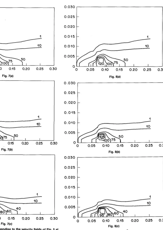
Fig. 7 The isotherms corresponding to the velocity fields of Fig. 5 at .,

h = 2 W/m2C. Note that the coordinates origin Is moved to the edge of F i a- 8 S a m e a s Fi9- 7 b u t w i , h h = 3 w / m c- T h e »h e r m a l boundary

the board. The temperature drop across the board is significant only at , a v e r s,«"=ture Is evident wtih the 1 C isotherm arbitrarily representing

the module location. t n e e d9e °* «he layer.

Computation of the temperature field was obtained on a larger mesh which consisted of the mesh shown in Fig. 4 augmented to include the circuit board (Fig. 2). We found ex-tremely slow convergence for the temperature solution. With

T= 0 as a starting point, it takes about 3000 iterations to

con-verge. Convergence is assumed when the maximum change in

T per iteration is less than 10~5xTm„. A

criterion of 1 0_ 4x rr T

•* m a x '

The variation of Tmax with U, at a pair of typical values for

h is given in Fig. 6. As expected, Tmax drops as U increases at

fixed h, or as h increases at fixed U. The power dissipation for all cases in Fig. 6 is fixed at 1 Watt. In all the cases considered,

max. ,* convergence

causes about an 8 percent error in

the point of maximum temperature was found at the center of the interface between the chip and the air gap underneath. The fraction of heat carried away by the cooling air is found to in-crease from 53 percent at (7=0.5 m/s and h = 3 W/m2C to 71

percent at U= 2 m/s and h = 2 W/m2C. The remainder is

car-ried away by free convection from the lower surface of the cir-cuit board.

The level of the maximum temperature Tmax in Fig. 6, while

realistic, is still too high. Typical values range from 40 to 130 C/W [3]. The assumed two-dimensionality over a depth dza is the main reason for these high values. Thus, TmSLX values from

Fig. 6 represent an unreachable upper bound. However, one is seldom concerned with a single module. If we are to use these

similar modules perpendicular to the direction of air flow with module spacing L, then a lower bound for rmax per Watt at a

given air velocity, would be that from Fig. 6 times (dza/L). With a L value of about 0.05 m, this means that the estimated temperatures will exceed one seventh but will not reach the values of Fig. 6. The need for fully three-dimensional model-ing, or some empirical correction for three-dimensional effects is evident. Another contributing factor to these high values of !Tmax is the assumed free convective lower surface. It is evident

from Fig. 6 that Tmm is sensitive, as expected, to the value of

h. In practice, the lower surface represents the upper boun-dary to another channel. Thus it is expected that a forced con-vective, although not uniform, situation to prevail at the lower boundary.

The isotherms corresponding to the three values of U with h = 2 W/m2C are shown in Fig. 7, while those with h = 3

W/m2C are in Fig. 8. The observed spread of the temperature

upstream is due entirely to the copper layers on the circuit board (Fig. 2). Thus while heat flows to the board at the module location, it flows from the board to the cooling air upstream of the module. The thermal boundary layer struc-ture is evident, in particular at the upstream edge of the module, with the 1°C isotherm arbitrarily representing the edge of the boundary layer. This thermal boundary layer is in-sensitive to the adiabatic boundary condition (Ad) as con-firmed from computations with a convecting top boundary. Careful study of Figs. 7 and 8 leads to the conclusion that there is no obvious way of arriving, a priori, at a "local air temperature" or an "average coefficient of heat transfer" at the module location. This shows the importance and the need for accurate conjugate heat-transfer modeling.

Concluding Remarks

Solution of the conjugate heat transfer problem which models forced air cooling of electronic devices has been presented. The ability to study the influence of particular change in design on the temperature distribution is demonstrated. For example, it is a straightforward matter to assess the consequences of replacing the air in the gap underneath the silicon chip by a more thermally conductive gas or, perhaps, a solid material. Indeed, many such studies can be carried out without having to recompute the flow field. Typical air velocities encountered in practice lead to flows

which are in the transitional regime, thus we assumed laminar conditions. However, the higher dissipation densities an-ticipated, forced air cooling at higher velocities will be needed. A turbulence model would then be required. The major weakness of the model lies in the assumed two-dimensionality. This is especially important if one is concerned with the per-formance of a single module. However, our results should be useful in the thermal design for a row of heat dissipating modules perpendicular to the direction of air flow. The varia-tion of the thermal conductivities with temperature may also have an appreciable influence in view of the sharp gradients encountered. Other related situations which are yet to be studied include rows of modules along the direction of air flow on one board, as well as rows of printed circuit boards perpen-dicular to the direction of air flow which would eliminate the need for including the somewhat artificial free-convective lower boundary. With the temperature distribution deter-mined, one can compute the thermal stresses due to differen-tial expansion within the package.

Acknowledgment

This work was performed in the Summer of 1983 while A. Zebib was a Faculty Participant at AT&T Bell Laboratories, Holmdel, New Jersey. We wish to acknowledge E. Y. Chen and G. P. Lowery for their assistance and many informative discussions. The paper was prepared for publication while A. Zebib was a visitor at Stanford University. The kind hospitali-ty of Professor G. M. Homsy is gratefully acknowledged. References

1 Steinberg, D. S., Cooling Techniques for Electronic Equipment, Wiley-Interscience, 1980.

2 Hannenman, R., "Microelectronic Device Thermal Resistance: A Format for Standardization," 1981 ASME Winter Annual Meeting.

3 Arvizu, D. E., and Moffat, R. J., "Experimental Heat Transfer From an Array of Heated Cubic Elements on an Adiabatic Channel Wall," Report no. HMT-33, Stanford University, 1981.

4 Sparrow, E. M., Niethammer, J. E., and Chaboki, A., "Heat Transfer and Pressure Drop Characteristics of Arrays of Rectangular Models Encountered in Electronic Equipment," Int. J. Heat Mass Transfer, Vol. 25,1982, pp. 961-973.

5 Patankar, S. V., Numerical Heat Transfer and Fluid Flow, Hemisphere Publishing, Washington, D. C , 1980.

6 Moffatt, H. K., "Viscous and Resistive Eddies Near a Sharp Corner," J.

FluidMech., Vol. 18, 1964, pp. 1-18.

7 Patankar, S. V., "A Numerical Method for Conduction in Composite Materials, Flow in Irregular Geometries and Conjuate Heat Transfer," Proc.

6th Int. Heat Transfer Conf., Toronto, Vol. 3, 1978, pp. 297-302.

Journal of Electronic Packaging MARCH 1989, Vol. 111/45