Porosity Gradient Gels pdf

Hunkapiller MW, Lujan E, Ostrander F and Hood LE (1983) Isolation of microgram quantities of proteins from polyacrylamide gels for amino acid sequence analysis.Methods in Enzymology91: 227.

Laas T (1989) Electrophoresis in gels. In: Janson J-C and Ryden L (eds) Protein PuriTcation } Principles, High Resolution Methods and Applications. New York, Weinheim and Cambridge: VCH Publishers.

Laemmli UK (1970) Cleavage of structural proteins during the assembly of the head of bacteriophage T4.Nature

227: 680.

Matsudaira PT and Burgess DR (1978) SDS microslab linear gradient polyacrylamide gel electrophoresis.

Analytical Biochemistry87: 386.

Schagger H and von Jagow G (1987) Tricine-sodium dodecyl sulfate}polyacrylamide gel electrophoresis for

the separation of proteins in the range from 1 to 100 kDa.Analytical Biochemistry166: 368.

Shapiro AL, Vinuela E and Maizzel Jr JV (1967) Molecular weight estimation of polypeptide chains by electrophor-esis in SDS-polyacrylamide gels.Biochem. Biophys. Res. Commun. 28: 815.

Takano E, Maki M, Mori H, Hatanaka N, Marti T, Titani K, Kannagi R, Ooi T and Murachi T (1988) Pig heart calpastatin: identiRcation of repetitive domain structures and anomalous behaviour in poly-acrylamide gel electrophoresis. Biochemistry 27: 1964.

Weber K, Pringle JR and Osborn M (1972) Measurement of molecular weights by electrophoresis on SDS-acrylam-ide gel.Methods in Enzymology26: 3.

Polyacrylamide Gel Electrophoresis

See II / ELECTROPHORESIS / One-dimensional Polyacrylamide Gel Electrophoresis; II / ELECTROPHORESIS / One-dimensional Sodium Dodecyl Sulphate Polyacrylamide Gel Electrophoresis;

II / ELECTROPHORESIS / Two-dimentional Polyacrylamide Gel Electrophoresis

Porosity Gradient Gels

G. M. Rothe, Johannes Gutenberg-University, Mainz,

Germany

Copyright^ 2000 Academic Press

Introduction

The high resolving power of polyacrylamide (PA) gels for proteins, peptides and nucleic acids can be im-proved by using gradient gels instead of homogene-ous (i.e. single concentration) gels. However, a more speciRc separation of polynucleotides in PA gels af-fords separation by incorporating a 40}80% de-naturant gradient (7 mol L\1_{urea, 40% (v/v)} form-amide) into a homogeneous PA gel (of e.g. 6.5% (w/v) total polymer concentration) or applying a tem-perature gradient to a homogeneous PA gel.

In PA gradient gels the average pore radius de-creases with increasing gel concentrations, i.e. in the direction of the migrating protein (polynucleotide) bands. This results in a sharpening of the bands be-cause the molecules at the front of the moving band are slower than those at the rear. Because of this effect, gradient gels need not be covered by a stacking gel, as in disc gel electrophoresis. In porosity gradient

gels with a steep increase of polymer concentration (e.g. from 4 to 30%T(w/v) where %T"g acrylam-ide#g Bis"N,N-methylenebisacrylamide (Bis) per 100 mL) proteins of a large size range (approximately 104_}106_{Da) can be separated. In shallow gradients} ('4% Tto(30%T), the separable size range of proteins is limited but they still provide an improved band sharpening.

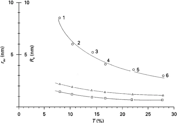
Figure 1 Plot of average pore radius (rav(nm)) against PA gel concentration (T (%)). Triangles, average pore radii calculated as

suggested by Ornstein and Davis (1962). Squares, average pore radii calculated as suggested by Raymond and Nakamichi (1962). Circles, maximum pore radii as marked by native proteins of known radius: 1, thyroglobulin; 2, ferritin; 3, catalase; 4, lactate dehydrogenase; 5, bovine serum albumin; 6, ovalbumin. Reproduced with permission from Rothe and Maurer (1986).

methods are employed when ultra-thin gels are to be used horizontally. Glass cassette cast PA gradient gels without any further support are used vertically.

Porosity of Polyacrylamide Gradient

Gels

In 1962 Ornstein and Davis were theRrst to suggest a formula to estimate roughly the average pore dia-meter of homogeneous PA gels:

pav(nm)"12.67;(%T)\1/2 [1]

where pav (nm) is the average pore diameter in nanometres and %Tis the total acrylamide concen-tration (g acrylamide#g Bis in 100 mL).

Based on the Ogston model which describes dex-tran gels as assembled from arbitrarily arranged gel

The largest pore diameter in a PA gel of a certain concentration is, however, much larger than the aver-age pore diameter (Figure 1). Moreover, the largest pore diameter deviates increasingly from the average pore diameter with decreasing gel concentration. The pores therefore are statistically distributed, but the standard deviations of the average pore radii and the distribution function (Gaussian or logarithmic distri-bution) are unknown.

Figure 2 Assembly of a glass cassette to cast a PA (gradient) gel slab. A, Slot former; B, front and D rear glass plate of cassette; C, left and right distance bar. 1, Exploded view of cassette; 2, side view; 3, front view. Procedure according to Pharmacia, Uppsala, Sweden. Reproduced with permission from Rothe (1991).

Analytical Separation of Native

Proteins in a Glass Cassette-Cast

Porosity Gradient

Gradient preparation is performed with acrylamide solutions of high and low concentrations, usually by using a two-chamber gradient mixer, although more sophisticated gradient formers have been developed. Linear PA gradients are usually prepared by the tech-nique which was_Rrst described by Martin and Ames in 1961 for the preparation of linear sucrose gradi-ents. Glass cassette-cast gels are mostly 82_;82 (140) mm or 125;250 mm and a thickness of 3.0, 1.0, 0.8, 0.5 or 0.1 mm.

Preparation of a Batch of Unattached Gradient Gels

Polyacrylamide gradient gels cast in glass cassettes may be prepared individually or simultaneously in batches (Figure 2). The latter method saves time and, although the gradients usually deviate slightly from each other, they are well suited to determine protein patterns, e.g. isozyme patterns as in population gen-etics. Any form of gradient (linear, concave, convex) may be prepared but linearly increasing gradients of total polymer concentration are most commonly used.

The device shown in Figure 3 can prepare six gradient gels simultaneously. In each gel the PA con-centration increases linearly from top to bottom from approximately 5 to 25%T. The gels are encased in glass cassettes of internal dimensions 172;82

;1.0 mm. Each cassette isRtted with a slot former and inserted in a gel-casting device. The linear PA gradient is prepared by using a two-chamber gradient mixer, a separate reservoir (for the catalyst solution), a proportioning pump, a 1 mL mixing chamber (and a reservoirRlled with sucrose and a pump to lift the gradient into the cassettes). The device shown in Figure 3 is used as follows: The inner chamber (1) and the connecting tube (3) to the outer chamber (2) of the gradient mixer are _Rlled with 57 mL of

Tminsolution. Then the tube (3) to chamber (2) of the mixer is closed. Afterwards 57 mL of theTmax solu-tion is pipetted into chamber (2) of the gradient mixer. Now 22.5L of N,N,N,N -tetra-methylethylenediamine (TEMED) is mixed with the

Tminand the Tmax solution, respectively. A separate reservoir (4) isRlled with 35 mL of gel buffer contain-ing 50 mg ammonium persulfate. The connection be-tween chamber (1) and (2) of the gradient mixer is opened, after which the stirrer (5) of the gradient mixer and the stirrer (6) of the mixing chamber (7) as well as the peristaltic pump (8) are switched on. Immediately after chamber (1) is empty, the pump (8) is switched off and a suf_Rcient amount of sucrose solution (50% (w_/v)) is pumped from the correspond-ing reservoir (9) with the help of a separate pump (10) underneath the gel cassettes (12) to lift the whole gradient into the cassettes, which are in the gel-cast-ing device (14).

TheTminandTmaxsolution contain acrylamide and Bis at the same ratio (acrylamide}Bis"24 : 1). The

Figure 3 (A) Device for preparing a batch of six PA porosity gradient gels. (B) Scheme for preparing a batch of six porosity gradient gels each encased in a glass cassette without further support. 1 and 2, chambers of the gradient mixer (1 with magnetic bar); 3, connecting tube between both chambers which can be closed by a stopcock (not shown); 4, reservoir to hold the catalyst solution (ammonium persulfate); 5 and 6, stirrers; 7, mixing chamber (modified 1 mL syringe); 8, two-channel pump; 9, reservoir to hold sucrose solution; 10, one-channel pump; 11, air trap; 12, gel cassettes with 13, inserted slot formers; 14, gel-casting apparatus (made of perspex) with 15 removable front plate. Reproduced with permission from Rothe (1994).

0.175 g Bis per 100 mL gel buffer while theTmax solu-tion contains 31.54 g acrylamide and 1.314 g Bis in 100 mL gel buffer. The Tmin and Tmax solutions are diluted upon gradient formation with catalyst tion by a factor of 1.255 (Figure 3) and the gel solu-tion is pumped to about 5 mm above the slot tem-plate. This results in a Rnal concentration range of approximately 5}25% T. (Mixing both catalysts into the Tmin and Tmax solution is also possible but carries the danger that the gel may solidify before being completely cast in the cassette). Prior to use all solutions are brought to room temper-ature and degassed. The ammonium persulfate solu-tion should be prepared freshly each time. 90 mmol L\1 _{Tris, 45 mmol L\}1 _{boric acid and} 2.5 mmol L\1_EDTA}Na

2, pH 8.4 is used as gel and electrode buffer. Further buffer systems are given in Table 1.

Vertical Electrophoresis

Table 1 Buffer systems used in porosity gradient gel electrophoresis to separate native proteins

Gel buffer Electrode buffer %Trange Authors

0.35 mol L\1_{Tris HCl, 0.06 mol L\}1_{, Tris, 3}20 KopperschlaKgeret al. (1969)}

pH 8.9 0.40 mol L\1_{glycine, pH 8.3}

0.09 mol L\1_{Tris, Same as gel buffer 4}26 Andersonet al. (1972)}

0.08 mol L\1_{boric acid, Lasky (1978)}

0.003 mol L\1_EDTA}Na 2,

pH 8.3

0.01 mol L\1_{Tris, Same as gel buffer 5}30 Slater (1969)}

0.08 mol L\1_{glycine, 5}15}

pH 8.3

0.04 mol L\1_{Veronal}Na, Same as gel buffer 5}30 Lambin and Fine (1979)}

0.04 mol L\1_Tris,

0.01 mol L\1_glycine,

0.04 mol L\1_{ethanolamine,}

0.001 mol L\1_EDTA}Na 2

pH 9.8

0.01 mol L\1_{Na}phosphate, Same as gel buffer 5}30 Lambin and Fine (1979)}

pH 7.2

References as given in Rothe and Maurer (1986). Reproduced with permission from Rothe and Maurer (1986).

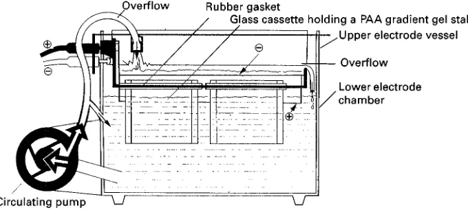
Figure 4 Vertical electrophoretic apparatus in which up to four glass cassette-cast porosity gradient gels can be inserted. Upper electrode vessel with 2 rubber gaskets to hold 2 to 4 glass cassettes, each containing a porosity gradient made of PA;#,!, electrodes. Modified from an instruction leaflet published by Pharmacia, Uppsala, Sweden.

PA gradient gel electrophoresis under nondenatur-ing conditions has proved to be advantageous com-pared to electrophoresis in homogeneous gels, e.g. in plant population genetics. Figure 5 gives an example.

Separation of Native Proteins in

an Ultra-Thin Support-Bound Porosity

Gradient

To prepare a thin gradient gel of the dimensions 120;250;0.5 mmRxed to a derivatized clear and Sexible polyester foil (e.g. manufactured by Gel

Bond, Marine Colloids, Rockland, MN, USA or Serva, Heidelberg, Germany), the gel-forming devices shown inFigure 6may be used. (When the cassettes are assembled the slot formers must not touch the opposite glass wall but leave a space of 0.1 mm in between). The following solutions may be used to form a gradient ranging from 3 to 30%T:

1. gel buffer: 90 mmol L\1_{Tris, 80 mmol L\}1_boric acid, 2.5 mmol L\1_{EDTA}Na2, pH 8.4;}

2. electrode buffer: 1 in 2 diluted gel buffer; 3. stock acrylamide solution (30%T: 28.8 g

Figure 5 Electrophoresis of plant diaphorase isoenzymes in a 4}20%T PA gradient gel of 0.8 mm thickness (length 175 mm, height 75 mm). (A) Zymogram of diaphorase enzymes (numbers indicate genotypes of the tetrameric enzyme at locus B. (B) Schematic representation of genotypes at locus DIA-A and DIA-B. Enzyme source: leaf buds of seven different trees of European beech (Fagus sylvatica L.). Conditions of electrophoresis: gel and electrode buffer: 45 mmol L_\1_{Tris, 40 mmol L\}1 _{boric acid, 1.25 mmol L\}1

EDTA}Na2; pH 8.4; running time 4 h; voltage gradient 40 V cm\1; temperature 53C.

Enzyme extraction: 1.5 mL Eppendorf tubes containing 150 mg of green bud leaves, 50 mg of quartz sand and 600L of extraction medium were cooled from underneath with ice water. A motor-driven grinding cone adapted in the shape of the tube (rotating at 700 rpm) was used to homogenize the material. The extraction medium contained in 100 mL: 1.21 g Tris, 1.43 g Na2HPO4, 60 mg

L-cysteine, 210 mg ascorbic acid, 14 g sucrose, 40 mg NADP, 15 g polyclar AT (PVPP) and 1 g polyethylene glycol, pH 7.5 (with H3PO4). The homogenate was centrifuged for 30 min at 43C and 10 000 g and the clear supernatant used as crude enzyme extract.

Samples of 8L were applied per lane. Diaphorase isozymes were visualized histochemically (60 mL 25 mmol L\1_{Tris-HCl, pH 8.5,}

containing 24 mg NADH, 1.5 mg 2,5 dichlorphenolindophenol-Na;2H2O (DCPIP) and 1.8 mL MTT (500 mg 100 mL\1aq. bidest.

water). Anode at bottom. A, Enzymes of gene locus DIA-A; B, locus DIA-B. In (A) not all genotypes indicated in (B) are shown.

4. dense acrylamide solution (30% T: to 6.5 mL stock solution is added, shortly before use, 20L TEMED (1 in 10 with H2O diluted solution) and 5L ammonium persulfate solution (40% w/v in distilled water));

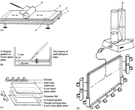
Figure 6 Preparation of an ultra-thin PA gradient gel fixed to a polyester foil. (A) Rolling the polyester foil (reactive side up, e.g. Gel Bond) on to one of the glass plates used to build the casting glass cassette: 1, levelling table; 2, glass plate; 3, hydrophilic side of polyester foil; 4, water layer; 5, rubber roller. (B) Trough template preparation. The bars are prepared from two layers of self-adhesive tape with a scalpel. (C) Assembling the glass cassette to cast the PA gradient. (D) Casting the porosity gradient: two-chamber mixer and glass cassette. Reproduced with permission from Rothe (1991).

solution (40% w_/v in distilled water) is added. The gradient is made of 6.5 mL of dense acrylamide solution and 6.5 mL of light acrylamide solution. After gradient formation, 2 mL of light acrylamide solution is overlaid; the slots must be situated in the middle of the 3%Trange.

Horizontal Electrophoresis

Before electrophoresis, the gel is taken out of the cassette. A few drops of kerosene are put on the cooling plate of the opened electrophoretic apparatus (Figure 7) and the gel,_Rrmly adhering to the polyes-ter foil, is placed on it, carefully avoiding the inclu-sion of air bubbles. Both ends of the gel are connected with the buffer vessels by paper wicks or a household sponge-like material. A 15}30 min

pre-electrophor-esis is performed at 1000 V (50 V cm\1_{). Then the} slots are Rlled with protein solution (or electrode buffer) and the power is turned on again at a voltage of 1000 V for approximately 2 h. Afterwards the gel, Rxed on the polyester foil, may be stained for proteins or (iso)enzymes (Figure 8).

Determination of the Course and

Concentration of a Porosity

Gradient Gel

Figure 7 Horizontal electrophoretic apparatus with cooling plate. 1, Cover lock; 2, gassing stud; 3, high voltage connection of the lid; 4, flexible tube to the cooling plate; 7, with a cooling device (not shown); 5, electrode bar (used in isoelectric focusing); 6, electrode ledge; 8, support for cooling plate. For PA gradient gel electrophoresis the electrode bars are replaced by two buffer vessels (not shown) under the cooling plate and connected to the electrode ledge. The gel is connected to the buffer reservoirs by (paper) wicks (not shown). Reproduced with permission from Rothe (1991).

Figure 8 Electrophoresis of plant (iso)enzymes on ultra-thin PA gradient gels fixed on a polyester film. Gel dimensions: 240;120;0.5 (mm); PA gradient from 4 to 28%T. Enzyme source: current-year (1989) needles of Norway spruce (Picea abies L., Karst.) sampled from a variety of clones (clone numbers indicated) of the multiple clone variety East Prussian Late Spruce (Hessische Forstliche Versuchsanstalt, Hann. MuKnden, Ger-many). Enzyme extraction: 2 g of fresh needles was homogen-ized in 10 mL of homogenizing medium (0.1 mol L\1_Na}

phos-phate, pH 7.5, containing 5% w_/v Polyclar AT and 0.5% w_/v Triton X-100. The crude extract was centrifuged for 30 min at 38 000 g and the supernatant concentrated by a factor of 4 using the ultrafiltration system Centrisart I (Sartorius, Go_Kttingen, Ger-many). Samples of 10L were applied per lane. Conditions of electrophoresis: 1000 V for 90 min at 43C; gel and electrode buffer: 45 mmol L\1_{Tris, 40 mmol L\}1_{boric acid, 1.25 mmol L\}1

EDTA}Na2, pH 8.4. Enzymes were stained histochemically.

An-ode at top. Reproduced with permission from Rothe (1991). intensity from top to bottom of the gel can be used to

measure the course of the gradient and its precise concentration in polyacrylamide. For a 1 mm thick gel 15 mgp-nitrophenol may be added to 100 mL of the dense acrylamide solution. After gelation the col-our intensity is quantiRed by densitometry at 405 nm. Whilst the course of the gradient can be seen directly on the densitogram, the %Trange of the gradient can be calculated with the formula:

T(%)"Ts;(E405!Ep);Mr;(c;d;)\1 [4]

whereTs(%) is PA concentration of stock solution,

E405is absorbance ofp-nitrophenol,Epis absorbance of empty cassette at 405 nm, c(g L\1_{) is} concentra-tion of p-nitrophenol in stock acrylamide solution (c"0.150),Mr(g L\1) is mol mass ofp-nitrophenol (Mr"139.1),d (mm) is thickness of gel (e.g. 0.5),

E [L (mol mm)\1_{]"molar extinction coefRcient of}

p-nitrophenol at 405 nm ("1728) andT(%), as in eqn [1].

Cross-Linkers Other than Bis and

Mixed Polyacrylamide Gels

acid or dilute aqueous solutions of bases to liberate proteins after the electrophoretic separation. Gradi-ent Sat gels (140;120;3 mm) with an increasing acrylamide concentration but a constant ratio of DHEBA have been used to separate protein mixtures from fruit with radio-labelled amino acids. Following electrophoresis, gel slices containing protein zones are placed in a glass scintillation counting vial Rtted with a TeSon-lined plastic cap, 1 mL of 0.025 mol L\1_{periodic acid is added and the vials are} sealed. After incubation for 48 h at 50₃C, 10 mL of Mix I scintillation_Suid is added, and the vials cooled overnight before counting. PA gels produced with DHEBA may be used with the common alkaline buf-fer systems except borate bufbuf-fers, which form nega-tively charged complexes with thecis-1, 2-diol struc-ture of the cross-linker DHEBA.

To improve the retardation of PA gradient gels for low molecular mass proteins, a mixture of acryl-amide, Bis and N,N,N-triallylcitric triamide has been suggested.

The use of N-substituted acrylamido derivatives, such as N-acryloyltris(hydroxymethyl)aminomethane (NAT) gives PA gels with larger pores, although the pores are still smaller than those of agarose. Gels of similar pore sizes can be made from allyl-activated agarose and acrylamide orN-substituted acrylamido derivatives. The mixed-bed gels of agarose} acrylam-ide have average pore sizes which are about 30% larger than those of a regular 3.3% Bis cross-linked gel with the same %T.

Size Estimation of Native Proteins and

Enzymes

The size of native proteins can be deduced from their migration behaviour in homogeneous or gradient gels. Both methods have the advantage that crude tissue or cell extracts can be used as the protein source, provided a speciRc staining method exists with which they can be located in the gel after elec-trophoresis. The method with homogeneous gels uses a number of gels of different PA concentration in the range of 4}35% T and estimates the relative elec-trophoretic mobility referred to Bromophenol blue (RFvalue) of a set of marker proteins and the sample protein(s). From these values the gel concentration is estimated at which the electrophoretic mobility is zero (or would become zero). This is achieved by plotting the logarithm of the %T concentration (logT) in which the mobility is measured against the respective RFvalue. In the underlying linear function (logT_"!k_;RF#logTlim), the value of Tlim rep-resents the exclusion limit, the %T concentration at which protein mobility stops. TheTlimvalues

cal-culated for a number of marker proteins can be corre-lated to their corresponding Stokes radii (RS) to ob-tain a calibration line. A linear function is obob-tained when RS is plotted against the reciprocal of

Tlim (RS"a;1/Tlim#b). Into this equation the ex-clusion limit of a sample protein is inserted and this then allows calculation of the corresponding Stokes radius.

Polyacrylamide gradient gel electrophoresis can also be used to estimate the molecular size of nondenatured proteins, provided it is performed in a time-dependent way. The following physicochemical properties of na-tive proteins (enzymes) are obtainable:

1. molecular mass (Mr);

2. hydrodynamic radius (Stokes radius (RS)); 3. frictional coefRcient (f/fo) (molecular eccentricity,

considering the molecular shape as a rotational ellipsoid and f/fo as the quotient of the ratio of the two half axes of the rotational ellip-soid, f"half axis of ellipsoid, fo"half axis of circle);

4. isomeric nature of multiple protein forms (size isomers or charge isomers);

5. free electrophoretic mobility (and nett negative charge (valenceZ, chargeQ)) at the pH value of the electrophoresis.

The mathematical procedures used to calculate these parameters are bound by several preconditions:

1. The PA gradient increases linearly (at a constant ratio of acrylamide to Bis). The gradient range however, can be chosen freely.

2. The electrophoretic pH value and the voltage gradient are chosen in a way that marker and sample proteins migrate sufRciently.

3. The same buffer system has been used as gel and electrode buffer, if net charges are to be obtained. 4. The sizes of the marker and sample proteinsRt the

pore range of the PA gradient.

5. Marker and sample proteins have migrated on the same gel slab.

6. Parts of the gel slab which have been cut into two or more parts and stained differently are re-equi-librated to the original gel length before protein migrations are measured.

7. Approximately 10 (or more) time-dependent mi-gration distances of marker and sample proteins are accurately measured.

Estimation of the Maximum Migration Distance and Recognition of Size Isomers

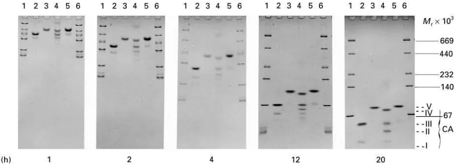
Figure 9 Time-dependent migration patterns of marker proteins and carbonic anhydrase (EC 4.2.1.1) (iso)enzymes from mam-malian erythrocytes. Lanes 1 and 6, marker proteins. Lanes 2}5; carbonic anhydrases from (2) bovine, (3) human, (4) rabbit and (5) canine. Mol mass of marker proteins: ovalbumin (45 000), bovine serum albumin (67 000), lactate dehydrogenase (140 000), catalase (232 000), ferritin (440 000) and thyroglobulin (669 000). Linear PA 4}30%T gradient (acrylamide}Bis"24 : 1), 300 V per 73 mm of gel length, 53C. Running times: 2, 8 and 16 h. Gel and electrode buffer: 90 mmol L\1_{Tris, 80 mmol L\}1_{boric acid, 1.25 mmol L\}1

EDTA}Na2}H2O, pH 8.4. Protein staining with Coomassie brilliant blue. Enzyme preparations from Sigma, Munich, Germany.

Reproduced with permission from Rothe (1991).

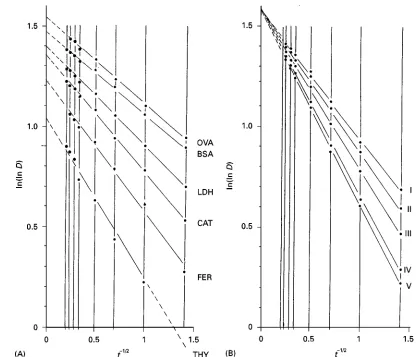
Migration of globular proteins comes to an end when the maximum pore size of a gel region equals their own size. The corresponding migration distance is called the maximum migration distance (Dmax (mm)). The maximum migration distance can be ob-tained from a number of time-dependent protein migrations (D (mm)) (Figures 9 and 10) which are directly measured on the gel after proteins have been visualized following electrophoretic separation (Table 2). To obtain the maximum migration dis-tance of a certain protein, the following mathematical approximation procedure can be applied: the migra-tion distances are double-logarithmized (ln(lnD)) and plotted versus the reciprocal of the square root of electrophoretic migration time, 1_/t1/2 _{(t (h)). This} results in a straight line (Figure 11) whereby the transformed migration values (ln(lnD)) and the transformed times of electrophoresis (t\1/2_{) are} inter-related by the equation:

ln(lnD)"!a;t\1/2_{#b [5]}

where a and b are the slope and the intercept of the corresponding straight line. The equation pre-dicts that at very high values of t, t\1/2 _reaches zero. This means that the maximum migration of a protein (Dmax(mm)) can be taken from the intercept of the straight line with the ordinate in a plot of ln(lnD) versus t\1/2 _{provided protein migrations} were larger than 2 mm and a suf_Rcient number of different migration distances are registered. Let-ting t approximate to inRnity means that eqn [5]

becomes:

ln(lnD)_"ln(lnDmax)"b [6]

and:

D"Dmax"exp(eb) [7]

A plot of ln(lnD) versus t\1/2 _{can also be used to} distinguish size isomers from charge isomers. Equally sized but differently charged forms of an enzyme or protein system are recognized by the fact that the straight line of each enzyme form intersects at the same point on the ln(lnD) axis as is for example the case with mammalian carbonic anhydrase (cf. Fig-ure 11) and mammalian lactate dehydrogenase. On the other hand, migration of charge isomers should result in lines of equal slope. Proteins differing in charge and size, however, give straight lines with both different slopes and intercepts.

Estimation of Stokes Radius and Molecular Mass

The maximum migration distance of globular pro-teins is related to the maximum gel pore radius at the respective gel concentration (cf.Figure 1). Therefore, the maximum migration distances (Dmax) of proteins can be correlated to their Stokes radius (RS). A linear relationship is obtained if the logarithm of the max-imum migration distance (lnDmax) of proteins is plot-ted versus the logarithm of their Stokes radius (lnRS):

Figure 10 (A) Plot of migration distances (D (mm)) of marker proteins and (B) of five different carbonic anhydrases versus times of electrophoresis (t (h)) in a linear PA gradient gel of 4}30%T. Conditions of electrophoresis are given in Figure 9. Migration distances and times of electrophoresis as listed in Table 2. OVA, Ovalbumin; BSA, bovine serum albumin; LDH, lactate dehydrogenase; CAT, catalase; FER, ferritin; TYR, thyroglobulin. Marker proteins and carbonic anhydrases were migrated on the same gradient gel. Purified enzyme preparations (Sigma, Munich, Germany) comprised carbonic anhydrases from bovine (I_}III), rabbit (III, IV), human (V) and canine (V) erythrocytes.

(Reproduced with permission from Chrambachet al. Advances in Electrophoresis Vol 4: pp 351I358.)

where lnDmaxequalsebof eqn [7], andmandb rep-resent the slope and intercept of the straight line (Figure 12).

It has been shown that a similar equation correlates the logarithm of the maximum migration distance (lnDmax) to the logarithm of the molecular mass (lnMr):

lnDmax"!z;lnMr#c [9]

where lnDmaxequalsebof eqn [7], andzand c rep-resent the slope and intercept of the straight line (Figure 12).

Knowing the maximum migration distance of any native globular protein, the calibration line can be used to calculate the molecular mass of the protein by inserting the calculated lnDmaxvalue and the values of the slope (z) and the intercept (c) of the calibration line into the equation lnDmax"!z;lnMr#c (Table 3) or inserting the lnDmaxvalue and the values of the slope (m) and the intercept (b) of the cali-bration line into the equation lnDmax"!m; lnRS#b(Table 4).

When using PA gradients of 4}30%Tand a buffer of pH 8.4 (45 mmol L\1 _{Tris, 40 mmol L\}1 _boric acid, 1.25 mmol L\1_{EDTA}Na2, pH 8.4) a number} of markers can be used, ranging from carbonic an-hydrase (Mr 30 000, RS 3.05) to thyroglobulin (Mr 669 000, RS 8.50; Table 5). -Galactosidase (Mr 116 000,RS4.23) and carbonic anhydratase (Sigma, St Louis, MO, USA) are run in the same lane and the other marker proteins are run in a separate one. The marker proteins bovine serum albumin, lactate de-hydrogenase, catalase, ferritin and thyroglobulin can be obtained as a freeze-dried mixture (Amersham Pharmacia Biotech, Freiburg, Germany) and dis-solved in a solution of pure ovalbumin (Boehringer, Mannheim, Germany). Separation times depend on the voltage gradient and may range from 0.5 to more than 20 h (Table 2).

Estimation of Frictional Coef\cient

The frictional coef_Rcient (f_/fo) relates the hydro-dynamic volume of a protein molecule to its molecu-lar mass. According to Siegel and Monty, the Stokes radius (RS) of a protein is related to its molecular mass (Mr) by the following equation:

RS(m)"f/fo;(3;;Mr)1/3;(4;;NA)\1/3 [10]

whereRS(m) is the Stokes radius,f/fois the frictional coefRcient (equivalent to the quotient of the half axes of a rotational ellipsoid), (m3_g\1_{) is the partial} speciRc volume (the reciprocal of the average density of a protein, ("0.75;10\6_{), N}

A (mol\1) is Avogadro’s number (NA"6.022;1023), and Mr (Da_"g mol\1_{) is the molecular mass of a protein.} By substituting the actual values one obtains:

RS(m)"f/fo;66.1;10\12;M1r/3 [11]

Figure 11 Plot of transformed migration distances (ln(lnD)) against transformed migration times (t_\1/2_{) of (A) marker proteins and}

(B) five carbonic anhydrase variants. Migration distances and times of electrophoresis as listed in Table 2. Abbreviations as in Figure 10. The common point of intersection of the various straight lines marked I}V on the ln(lnD) axis indicates that the investigated enzymes are size isomers. Reproduced with permission from Rothe (1991).

by settingf/fo"1 in eqn [11] to give eqn [12]:

RS(m)"66.1;10\12;M1r/3 [12]

This means that RSandRmare interrelated through the frictional coefRcient:

RS"f/fo;Rm [13]

The frictional coefRcient can be obtained from the experimentally obtained Mr and RS values and eqn [13].

Extremely high frictional ratios are to be expected for molecules with rod-like or Rbrous structures, which are characterized by a high axial ratio such as Rbrinogen or myosin or by bulky and voluminous globular molecules with normal axial ratios. Exam-ples of the latter are the spider-like immunoglobulin M, the shell-like apoferritin or the branched -macro-globulin. Usually, native proteins and enzymes do not belong to these groups of proteins.

In eqn [11] the frictional coefRcient of native pro-teins is assumed to be constant. However, when analysing the molecular mass (Mr) and Stokes radius (RS) of more than 60 native proteins it became apparent that the frictional coefRcient increases with increasing protein size (see Further Reading). A more precise equation relatingRSandMris the following:

RS(m)"M0.0225r ;55.1;10\12;M0.0142r ;M1r/3 [14]

According to this expression the frictional coefRcient of globular proteins equals f/fo"M0.0225r and in-creases with molecular masses of 103_{to 9;10}6_from

f/fo"1.17 tof/fo"1.43 while the factor 66;10\12 of the expression of Siegel and Monty (RS(nm)"f/fo;66.1;10\12;M1r/3) increases from 61_;10\12_{to 67;10\}12_.

Table 2 Time-dependent migration distances of marker proteins and carbonic anhydrase (iso)enzymes from erythrocytes of four mammalian species in a porosity gradient gel from 4 to 30%T

Protein Time t (h) of electrophoresis (1_/(t given in brackets)

0.5 1 2 4 8 12 16 20

(1.41421) (1.00000) (0.70711) (0.50000) (0.35355) (0.28868) (0.25000) (0.22361)

Ovalbumin D (mm) 13.05 20.25 31.5 44.0 54.0 61.0 67.5

Bovine serum albuminD (mm) 11.7 17.8 26.5 36.3 43.5 47.5 50.5 53.2

L-lactate D (mm) 7.5 11.9 17.5 24.5 30.2 33.3 35.5 37.5 dehydrogenase

Catalase D (mm) 5.5 8.8 13.2 18.8 23.5 26.6 28.5 30.0

Ferritin D (mm) 3.7 6.5 9.0 12.0 14.3 16.6 17.9 18.9

Thyroglobulin D (mm) 1.9 3.5 4.7 6.5 8.0 10.0 10.8 11.6

Bovine I D (mm) 7.3 12.5 21.5 35.5 48.2 56.0 62.5

Bovine II D (mm) 6.3 11.0 19.0 32.5 45.0 52.3 58.8 68.0

Bovine, rabbit III D (mm) 5.0 8.8 15.5 27.5 40.1 47.5 52.0 58.0

Rabbit IV D (mm) 3.8 6.7 11.8 21.5 33.6 41.0 45.7 50.2

Canine, Human V D (mm) 3.5 6.3 11.2 20.0 32.5 39.8 44.5 48.5

D (mm), Time-dependent migration distances of marker proteins and carbonic anhydrase (EC 4.2.1.1) variants. Gel length (D (mm)) and gel concentration (T (%)) are interrelated by the equationT_"D_#where"0.3528$0.0054 and"4.1116$0.2344; the correlation coefficient isr_"0.9985. Reproduced with permission from Rothe (1991).

Figure 12 Calibration lines to calculate the molecular mass (M) and Stokes radius (RS) of five carbonic anhydrase isoenzymes. The

logarithm of the maximum migration distance (lnDmax) correlates linearly to the logarithm of the mol mass (lnMr) and the logarithm of

the Stokes radius (lnRS), respectively. CA, Carbonic anhydrase (average lnDmaxof isozymes I}V); OVA, ovalbumin; BSA; bovine

serum albumin; LDH, lactate dehydrogenase; CAT, catalase; FER, ferritin; THY, thyroglobulin. The calculated mol masses and Stokes radii are listed in Tables 3 and 4.

500_}1000 kDaf_/fo"1.43. From these data and the Stokes radius of a globular protein its molecular mass can be estimated:

Mr"(1/(f/fo))3;3463;R3S [15]

withMr,f/foandRSas in eqn [10].

This can be exempliRed by mammalian liver alco-hol dehydrogenase (EC 1.1.1.1), which has a molecu-lar mass of 80 kDa and a Stokes radius of 3.5 nm; the

average frictional coef_Rcient of globular proteins in that range isf_/fo"1.23. By inserting these values into eqn [15] one obtains: Mr(Da)"(1/1.23)3;3463; 3.53_{"79 791.}

Determination of Migration Velocities

Bovine II 10.4904 35 968 4.8686

Bovine/rabbit III 38 000 10.5373 37 695 4.8387

Rabbit IV 10.5775 39 241 4.8131

Canine/human V 29 700 10.5462 38 032 4.8330

Arithmetic mean 10.5346 37 594 4.8404

a_{Literature values.}

b_{The molecular mass of bovine carbonic anhydrase as estimated by sequence analysis was reported to be 28 980 while that of the}

enzyme from mouse was found to be 29 068.

c_{The molecular sizes calculated are compared with the literature data and the percentage deviation indicated.}

Reproduced with permission from Rothe (1991).

Table 4 Calculated Stokes radius of marker proteins and mammalian carbonic anhydrase (iso)enzymes and calculation of percent-age of deviation of calculated values from the literature

Protein Stokes radius lnRS Calculated Stokes radius (RS) lnDmax

(RS(nm))a

lnRS RS Percentage

(nm) deviationb

Ovalbumin 3.05 !19.6081 !19.5992 3.08 #0.9 4.6563

Bovine serum albumin 3.55 !19.4563 !19.4285 3.65 #2.8 4.3537

L-Lactate dehydrogenase 4.20 !19.2881 !19.2590 4.32 #2.9 4.0532

Catalase 5.25 !19.0650 !19.1634 4.76 !9.3 3.8836

Ferritin 6.10 !18.9150 !18.8987 6.20 #1.6 3.4144

Thyroglobulin 8.50 !18.5832 !18.5668 8.64 #1.7 2.8259

Carbonic anhydrase

Bovine I !19.7070 2.76 4.8476

Bovine II !19.7189 2.73 4.8686

Bovine_/rabbit III _!19.7020 2.78 4.8387

Rabbit IV _!19.6876 2.82 4.8131

Canine_/human V _!19.6988 2.78 4.8330

Arithmetic mean !19.7030 2.77 4.8404

a_{Literature values.}

b_{The molecular sizes calculated are compared with the literature data and the percentage deviation indicated.}

Reproduced with permission from Rothe (1991).

intervals during electrophoresis, and the correspond-ing time difference:

v(mm s\1_)"(D

1!D0);(t1!t0)\1

v(mm s\1_)"(D

2!D1);(t2!t1)\1

v(mm s\1_)"(D

3!D2);(t3!t2)\1

v(mm s\1_)"(D

Z!DZ_\1);(tZ!tZ_\1)\1

Eqn [16] summarizes this procedure:

v(mm s\1_)"(D

n!Dm);(tn!tm)\1"dD;dt\1 [16]

Table 5 Marker proteins that can be used to estimate the native molecular size of proteins

Marker protein Mr RS

Carbonic anhydrase 30 000 2.43

Ovalbumin 45 000 3.05

Bovine serum albumin 67 000 3.55

-Galactosidase 116 000 4.23

Lactate dehydrogenase 140 000 4.20

Catalase 232 000 5.25

Ferritin 440 000 6.10

Thyroglobulin 669 000 8.50

Mr (Da), Molecular mass; RS (nm), Stokes’ radius of proteins.

These markers can be taken when using PA gradients of 4}30%

T and a buffer of pH 8.4 (45 mmol L\1_{Tris, 40 mmol L\}1_boric

acid, 1.25 mmol L\1_EDTA}Na

2, pH 8.4).

Correlating Migration Velocities and Migration Distances

The migration velocities may be plotted against the corresponding migration distances at the end of each time interval to correlate migration velocities and migration distances (Figure 13). The function by whichvandDare interrelated is best described by the following exponential equation:

v(mm s\1_)"(D

max!D)B [17]

where , Dmax and are constants, D (mm) is the independent variable and v(mm s\1_{) the dependent} variable. Dmax represents the maximum migration distance which a protein can cover, i.e. the migration distance at which the migration velocity becomes zero. If this point is reached thenDmax"D and:

v(mm s\1_{)"(D!D)B"0 [18]}

Eqn [17] can be used to relate the apparent migration velocity (v) of a protein to the PA concentration (T

(%)) that corresponds to the migration distance travelled during a given period of electrophoresis. When using a linear gel gradient, the PA concen-tration and the gel length are interrelated by eqn [19]:

D"\1_{(T!) [19]}

whilst Tmax (%), the stacking gel concentration, is related to the maximum distanceDmax(mm) by eqn [20]:

Dmax"\1(Tmax!) [20]

Substituting eqns [19] and [20] into eqn [17] yields the formula:

v(mm s\1_)"[((T

max!);\1)!((T!);\1)]B [21]

which can be arranged to:

v(mm s\1_)";\B;(T

max!T)B [22]

and:

v(mm s\1_)"h;(T

max!T)B [23]

whereh";\B.

This derivation shows that, indeed, the apparent migration velocity of a protein (v) is related by the same function to the distance (D) as to the PA concen-tration (T) it has reached in a linear pore gradient, although the constants ( and Dmax, respectively,

h and Tmax) are different. The exponent in both equations, however, is the same.

Eqn [23] predicts that zero protein mobility (v"0) results if the apparent gel concentration (T (%)) is equal to the stacking gel concentration (Tmax(%)), i.e. ifT"Tmax. The apparent free electrophoretic mobil-ity of a protein unhindered by the PA matrix ( (mm s\1_{)), can be calculated by simply extrapolating} its apparent mobility to zeroT(%):

(mm s\1_)"h;(T

max!0)B [24]

thus:

(mm s\1_)"h;TB

max [25]

This expression may be used to divide eqn [23] to yield eqns [26] and [27]:

v;\1_"(h;(T

max!T)B);(h;TBmax)\1 [26]

which can be rewritten as:

v"[1!(T;T\_max)]1 _{B [27]}

The value of the quotient (Tmax!T);T\max1 ranges from one (T"0) to zero (T"Tmax) and thus the value of v extends from the apparent free electro-phoretic mobility () to zero.

Figure 13 (A) Estimation of the migration velocity of a protein (OVA, ovalbumin) in a linear PA gradient gel.Tn, migration distance at

a longer time of electrophoresis (tn);Tm, migration distance at a shorter time of electrophoresis (tm). (B) Plot of the resulting migration

velocities (v (mm s_\1_{) versus the corresponding gel concentrations (T (%)) at the end of each time interval.}

values between zero and one and increases exponenti-ally with increasing gel concentrations.

In order to solve eqn [23] (v(mm s\1_)"h; (Tmax!T)B), the following sequence of calculations is recommended:

1. determination of the maximum migration distance of the protein under investigation from a plot of ln (lnD) vs.t\1/2 _{(eqn [5])}

2. computation of the maximum gel concentration (Tmax) by use of eqn [20] (Dmax"\1(Tmax!));

3. calculation of the gel concentration equivalent to the migration distances with eqn [19] (D" \1_{(T!)), (the values of the constants and}

may be obtained from a gel scan at 405 nm if

p-nitrophenol has been mixed into the more con-centrated of the two solutions used to prepare the gradient gel);

4. then the values of (Tmax!T) are calculated 5. _Rnally the constantsh and in eqn [23] are

Table 6 Free electrophoretic mobility (U ) and net negative charge (valence, Z ; charge, Q) of several marker proteins and carbonic anhydrase (iso)enzymes from mammalia at pH 8.4

Protein U (m2_{(V s)\}1_;10\9₎ Negative charge

I_"0.529_;103a

I_"0.1_;103b _{Z Q (C molecule\}1_);10\19

(mol m_\3₎

(mol m\3₎

Ovalbumin 3.45 5.99 13.06 20.92

Bovine serum albumin 4.40 7.85 22.42 35.92

Lactate dehydrogenase 3.27 6.00 22.63 35.25

Catalase 2.60 4.94 21.43 34.33

Ferritin 3.28 6.38 43.81 70.18

Thyroglobulin 2.78 5.62 68.46 109.67

CA I 1.58 2.69 4.93 7.90

CA II 1.17 1.99 3.58 5.74

CA III 1.05 1.79 3.32 5.32

CA IV 0.851 1.46 2.75 4.41

CA V 0.734 1.25 2.31 3.70

a_{Ionic strength of electrophoretic buffer system.}

b_{Free electrophoretic mobility at ionic strength 0.1;10}3_(m2_{(V s)\}1_).

CA, Carbonic anhydrase (iso)enzymes from mammalian erythrocytes: (bovine, I, II), bovine, rabbit (III), rabbit (IV) and canine, human (V). Conditions of electrophoresis: linear polyacrylamide gradient from 4 to 27%T (acrylamide}Bis"24 : 1); gel length 73 mm; buffer system 90 mmol L\1_{Tris; 80 mmol L\}1_{boric acid; 1.25 mmol L\}1_EDTA}Na

2, pH 8.4 (I"529 (mol m\3); field strength: 41 V cm\1;

43C.

Reproduced with permission from Rothe (1991).

i.e. taking the logarithmized version of eqn [23]:

lnv";ln(Tmax!T)#lnh [28]

Calculation of the Free Electrophoretic Mobility

The free electrophoretic mobility (U(m2_V\1_s\1_{)) of} a protein results from its apparent free electrophotetic mobility unhindered by the gel matrix ((m s\1_{)) and} the electric_Reld strengthE(V m\1_{) acting on it:}

U";E\1_{(m s\}1_{(V m\}1_)\1_"m2_V\1_s\1_{) [29]}

The apparent free electrophoretic mobility can be obtained by applying eqn [25] ((mm s\1_)"

h;Tmax). The free electrophoretic mobilities ofB various marker proteins and Rve different mam-malian carbonic anhydrases calculated by these pro-cedures are listed in Table 6.

Computation of the Nett Charge

Estimation of the number of unit charges (Z) in a nondenatured protein requires prior knowledge of its Stokes radius (RS) and its apparent free electro-phoretic mobility () or its free electrophoretic mobil-ity (U). In addition to this, the ionic strength (I) and viscosity ( ) of the buffer system used to estimate

Zand RSmust be known. Time-dependent gradient gel electrophoresis can be used to determine the Stokes radius of a protein and its free electrophoretic mobility.

At a Rrst approximation, the free electrophoretic mobility, unhindered by a gel matrix (U

(m2_V\1_s\1_{)), can be described by eqn [30]:}

U"(Z;);(6;; ;RS)\1

(C(Pa s m)\1_"m2_{(V s\}1_{) [30]}

whereZis the number of unit charges (1);is the unit charge (protonic charge)_"1.602_;10\19 _(C);

"3.14₂; is the dynamic viscosity of the medium (Pa s);RSis the Stokes radius (m) and the following coherences 1 C"1 A s, 1 Pa"1 N m\2_{, 1 V A"} 1 W and 1 W s"1 N m.

Figure 14 Graphical representation of Henry’s functionX1(RS). Depending on the value ofRSthree different equations must be

used to compute the values ofX1. IfRS'24 (case 1), the first of the three equations given is used. The second equation (case 2)

comes into use if 54RS424 while the third equation (case 3) is applied ifRS)5. In the latter case, Table 6 provides a number of

values. Reproduced with permission from Rothe (1991). The function X1(;RS) is complicated but always gives values between 1.0 and 1.5, as shown in Figure 14. According to Henry, three different equa-tions must be used to compute the values of the functionX1. If;RS'24 then theRrst of the three equations indicated in Figure 14 must be used. When

;RS)5 the last of the three equations inFigure 14 is applied. In the range between the two border values 5 and 24, a linear equation is taken, which is also

creases permanently in solutions with increasing salt concentrations. The value of kappa can be obtained from the equation:

"[(2NA;2)

;(D0;D;k;T)\1_]1/2_;I1/2_(m\1_{) [33]}

whereNA"6.025;1023(mol\1);is the unit charge (protonic charge)"1.602;10\19_(C);D

Table 7 Values of Henry’s function (X1(;RS)) if;RS(5 (cf. Figure 14)a

;RS log10(;RS) X1according to

Overbeek’s modification of Henry’s equation

;RS log10(;RS) X1according to

Overbeek’s modification of Henry’s equation

0.01 !2 1.0000062 1.95 0.2900346 1.0632127

0.05 !1.30103 1.0001452 2.00 0.30103 1.0651048

0.10 _!1 1.0005451 2.05 0.3117539 1.0669887

0.15 _!0.8239087 1.0011577 2.10 0.3222193 1.0688642

0.20 _!0.69897 1.001951 2.15 0.3324385 1.0707308

0.25 !0.60206 1.0028994 2.20 0.3424227 1.0725882

0.30 !0.5228787 1.003982 2.25 0.3521825 1.0744361

0.35 !0.455932 1.005181 2.30 0.3617278 1.0762744

0.40 !0.39794 1.0064817 2.35 0.3710679 1.0781027

0.45 !0.3467875 1.0078712 2.40 0.3802112 1.0799208

0.50 !0.30103 1.0093387 2.45 0.3891661 1.0817286

0.55 !0.2596373 1.0108744 2.50 0.39794 1.0835259

0.60 !0.2218487 1.0124701 2.55 0.4065402 1.0853126

0.65 !0.1870866 1.0141185 2.60 0.4149733 1.0870886

0.70 !0.154902 1.0158129 2.65 0.4232459 1.0888537

0.75 !0.1249387 1.0175476 2.70 0.4313638 1.0906078

0.80 !0.09691 1.0193175 2.75 0.4393327 1.0923509

0.85 !0.0705811 1.0211181 2.80 0.447158 1.094083

0.90 _!0.0457575 1.0229452 2.85 0.4548449 1.0958039

0.95 _!0.0222764 1.0247952 2.90 0.462398 1.0975136

1.00 0.0 1.0266648 2.95 0.469822 1.0992121

1.05 0.0211893 1.028551 3.00 0.4771213 1.1008994

1.10 0.0413927 1.0304511 3.05 0.4842998 1.1025754

1.15 0.0606978 1.0323626 3.10 0.4913617 1.1042402

1.20 0.0791812 1.0342836 3.15 0.4983106 1.1058938

1.25 0.09691 1.0362118 3.20 0.50515 1.1075361

1.30 0.1139434 1.0381455 3.25 0.5118834 1.1091672

1.35 0.1303338 1.0400832 3.30 0.5185139 1.1107871

1.40 0.146128 1.0420233 3.35 0.5250448 1.1123958

1.45 0.161368 1.0439644 3.40 0.5314789 1.1139934

1.50 0.1760913 1.0459054 3.45 0.5378191 1.11558

1.55 0.1903317 1.0478451 3.50 0.544068 1.1171554

1.60 0.20412 1.0497825 3.55 0.5502284 1.1187199

1.65 0.2174839 1.0517167 3.60 0.5563025 1.1202734

1.70 0.2304489 1.0536469 3.65 0.5622929 1.1218159

1.75 0.243038 1.0555723 3.70 0.5682017 1.1233477

1.80 0.2552725 1.0574921 3.75 0.5740313 1.1248686

1.85 0.2671717 1.0594059 3.80 0.5797836 1.1263788

1.90 0.2787536 1.0613129 3.85 0.5854607 1.1278783

3.90 0.5910646 1.1293672 4.45 0.64836 1.1450647

3.95 0.5965971 1.1308456 4.50 0.6532125 1.1464318

4.00 0.60206 1.1323134 4.55 0.6580114 1.1477892

4.05 0.607455 1.1337709 4.60 0.6627578 1.1491371

4.10 0.6127839 1.135218 4.65 0.667453 1.1504754

4.15 0.6180481 1.1366549 4.70 0.6720979 1.1518043

4.20 0.6232493 1.1380816 4.75 0.6766936 1.1531238

4.25 0.6283889 1.1394981 4.80 0.6812412 1.1544341

4.30 0.6334685 1.1409047 4.85 0.6857417 1.1557352

4.35 0.6384893 1.1423012 4.90 0.6901961 1.1570272

4.40 0.6434527 1.1436879 4.95 0.6946052 1.1583101

5.00 0.69897 1.159584

a_{Values were calculated using eqn [3] of Figure 14 (cf. Overbeek JTG (1950)Advances in Colloid Science, 3: 97}135). Tolerance of}

values: 10_\6_{, calculation of integral: 7 digits. Data from Rothe (1991).}

the dielectric constant of vacuum_"8.8542_;10\12 (C V\1_m\1_"C2_N\1_m\2_{); D is the} temperature-dependent dielectric constant of water (without dimension, cf. Table 8), k is Boltzmann’s

"[(2_;6.025_;1023_;(1.602;10\19₎2_);(8.8542 ;10\12_;1.3805;10\23_)\1_]1/2_{(K m (mol)\}1₎1/2 ;(I(D T)\1₎1/2_{(mol m\}3_K\1₎1/2 _[34] thus:

"1.590608013;1010_{(K m mol\}1₎1/2 ;(I(D T)\1₎1/2_{(mol m\}3_K\1₎1/2 _[35]

At a temperature of 53C (278 K), the dielectric constant of water is 85.90 (cf. Table 8). Inserting both values into eqn [35] yields eqn [36]:

"1.02930525;108_{(m mol\}1₎1/2

;(I(mol m\3₎1/2 _[36]

The ionic strengthI(mol m\3_{) is calculated using} the formula:

I"1/2ciZ2i(mol m\3) [37]

whereci(mol m\3) represents the concentrations of the ionic species of the buffer times their squared charges (Zi).

Taking , for example, a 90 mmol L\1_{Tris, 80 mmol} L\1_{boric acid, 1.25 mmol L\}1 _EDTA-Na

2buffer of pH 8.0, the ionic strength of this buffer is:

I_"1_/2ciZ2i (mol dm\3) [38]

thus:

I"1/2[(0.09;12_)#(3;0.08;12₎

#(0.08;(!3)2_{)#(2;0.00125;1}2₎

#(0.00125_;(_!2)2_{)] [39]}

which becomes:

I"0.52875 (mol dm\3_{) [40]}

Taking ferritin as an example, with a Stokes radius of 6.20_;10\9 _{(m), then;R}

S"14.67. The log of

;RSequals 1.167 and using this value one obtains from the equation in case 2 shown in Figure 14, a value of 1.293 for the function X1 (;RS). Thus, inserting these values into eqn [31], it follows that:

F"(X1(;RS));(1#(;RS))\1

"1.293;(1#14.67)\1_{"0.08251 [44]}

To calculate the number of nett charges in ferritin, eqn [32] must be solved forZ:

Z"((U;6;; ;RS);\1_);((1#(;RS))

;(X1(;RS))\1_{) [45]}

From gradient gel electrophoresis results, the free electrophoretic mobility of ferritin was calculated as

U"3.28;10\9_(m2_V\1_s\1_{). Substituting this value,} that of factorF and the value for the temperature-dependent dynamic viscosity ( (N s m\2_{)) of water} as taken from Table 9 into eqn [45], the number of unit charges that ferritin acquires under the electrophoretic conditions indicated above can be computed as:

Z_"(3.28_;10\9_{;6;;1.519;10\}3

;6.20;10\9_);(1.602;10\19_)\1 ;((1;0.08251)\1_{) [46]}

which works out to:

Z"44.05 [47]

Table 9 Dynamic viscosity ( (N s m\2_{)) of water depending on}

the temperature (t (3C))

t (₃C) (N s m_\2_{) 10\}3 _{t (3C) (N s m\}2_{) 10\}3

0 1.787 16 1.109

1 1.728 17 1.081

2 1.671 18 1.053

3 1.618 19 1.027

4 1.567 20 1.002

5 1.519 21 0.9779

6 1.472 22 0.9548

7 1.428 23 0.9325

8 1.386 24 0.9111

9 1.346 25 0.8904

10 1.307 26 0.8705

11 1.271 27 0.8513

12 1.235 28 0.8327

13 1.202 29 0.8148

14 1.169 30 0.7975

15 1.139

Reproduced with permission from West (1976}1977).

Table 10 Free electrophoretic mobility of ferritin in buffered solution

Experimental conditions Free mobility

U (m2_V\1_s\1_);10\9

Reference

Moving boundary method !6.1 Mazuret al. (1950)

I"0.1 (mol L\1_{), 0 (3C), pH 8.6}

Agarose gel electrophoresis !10.5 Goshet al. (1974)

I"0.05 (mol L\1_{),#20 (3C), pH 6.8}

Disc electrophoresis Rodbardet al. (1971)

C_"2%; 0 (3C), pH 8.88

I_"0.0034 (mol L\1_{) !10.97}

I_"0.10 (mol L\1_{) !5.67}

PA gradient gel electrophoresis Rothe (1991)

5_}30T (%), acrylamide_}Bis_"24 : 1;_#4 (₃C), pH 8.4a

I_"0.529 (mol L_\1_{) !3.28}

I"0.10 (mol L\1_{) !6.38}

a_{Electrophoretic conditions; 90 mmol L\}1_{Tris, 80 mmol L\}1_{boric acid, 1.25 mmol L\}1_EDTA}Na

2, pH 8.4; separation distance 73 mm,

voltage gradient 41.1 (V cm\1₎

References are given in Rothe (1991).

Evaluation of the Free Electrophoretic Mobility at an Ionic Strength of 0.1 mol L+1

For reasons of comparability, the free electrophoretic mobility obtained for a given set of experimental conditions may be corrected to an effective mobility at an ionic strength of 0.1 mol L\1_{. This can be} achieved by substituting the relevant values into Abramson’s equation:

U0.1"(U0.1(0.1;RS#2.4));(0.1;RS#2.4)\1 [48]

whereU0.1andU0.1(m2V\1s\1) represent the free electrophoretic mobilities at an ionic strength of 0.1 (mol m\3_{) and'0.1 (mol m\}3_{) respectively;}

0.1 and0.1represent the reciprocal of the effective thick-ness of the ionic cloud at ionic strength of 0.1 (mol m\3_{) and'0.1 (mol m\}3_{) respectively and}

RS(m) is the Stokes radius of the protein. For the experimental conditions given earlier:

0.1"1.02930525;108(m mol\1)1/2

;(0.1;103₎1/2_{(mol m\}3₎1/2 _[49]

thus:

"1.02930525;109_(m\1_{) [50]}

Taking ferritin as an example, for which U

(m2_V\1_s\1_)"3.28;10\9 _{(at I"0.529;10}3 (mol m\3_{), if}

0.1"2.366842604;109 and RS" 6.20;10\9_{(m) are determined and substituted into eqn} [48], it follows that:

U0.1"((3.28;10\9);(2.366842604;109;6.20 ;10\9_{#2.4));(1.02930525;10}9

;6.20;10\9_#2.4)\1 _[51]

thus:

U0.1"6.377;10\9(m2V\1s\1) [52]

v";[1!(T;T_max)]\1 _{B(m s\}1_{) [27]}

wherevis the migration velocity (m s\1_{),T(%) is the} PA concentration which the migrating protein of mo-bilityvhas reached andTmax(%) represents the exclu-sion limit of the migrating protein.

SinceU_";E\1_(m2_V\1_s\1_{), it follows that:}

v;E\1_{"U;[1!(T;T\max)]}1 _{B(m V\}1_s\1_{) [53]}

Uis deRned by eqn [32] as equivalent to:

U"(Z;);(6;; ;RS)\1_;(X1(;RS))

;(1#(;RS))\1_(m2_{(V s)\}1₎

with the deRnitions given above.

Using all this information, a complete description of the electrophoretic mobility of proteins migrating in a linear PA gradient gel can then be given by the equation:

v;E\1_{"(Z;);(6;; ;RS)\}1_;(X1(;RS))

;(1#(;RS))\1_{;[1!(T;T\max)]}1 _B(m2_{(V s)\}1₎ [54]

with the deRnitions as given above.

Sodium Dodecyl sulfate Porosity

Gradient Gel Electrophoresis

Polyacrylamide gradient gels also offer greater possi-bilities for the electrophoretic separation of proteins in the presence of SDS. Porosity gradient gels have a much higher resolving capacity, for example the two chains of haemoglobin of Mr"15 126 and 15 866 Da, respectively, can be clearly separated in a 3_}30% T gradient gel. An 8% T continuous PA}SDS gel does not exhibit this resolving capacity. In SDS porosity gradient gel electrophoresis the

by proteins after a certain time of electrophoresis. The validity of the corresponding relationship logMr"!a;logT#b has been conRrmed with some 40 proteins between 14 and 950 kDa. In PA gradient gels in the presence of SDS the molar mass of both unreduced and 2-mercaptoethanol-reduced proteins as well as the molar mass of glycoproteins can be determined with the same accuracy ($5%, Table 12). Ribonuclease and lysozyme binding normal amounts of SDS migrate anomalously in ho-mogeneous SDS gels but not in SDS PA gradient gels. Papain and pepsin, which also bind only traces of SDS, migrate regularly in SDS PA gradient gels.

The migration distance of proteins in linear SDS PA gradient gels and their respective mol mass can also be correlated by the equation:

logMr"!a;(D#b [55]

where D (mm) is the migration distance. This rela-tionship can be applied to SDS-complexed and re-duced and to SDS-complexed nonrere-duced proteins, to glycoproteins and to carbohydrate-free proteins (Figure 15). The relationship is not affected by the buffer system, the concentration of the cross-linker within 1_}8% C or the concentration range of the gradient within 3}30%Tat the commonly used gel length of 8}15 cm. The value of the constantsaandb, on the other hand, are changed when the experi-mental parameters are altered. If SDS electrophoresis is performed in a linear gradient gel of approximately 6}27% T, the relationship logMr"

Table 11 Gel and buffer systems used in SDS PA gradient gel electrophoresis to separate denatured proteins

PA range (%T ) (acrylamide_}Bis)

Gel shape (dimensions (mm))

Buffer systems

Gel buffer Electrode buffer

Current or voltage per gel Running time (h) Correlation (Mrrange

(kDa))

Notes Authors

3}30 (30 : 0.8)

Column (150_;6)

0.1 mol L\1

Na_}phosphate,

0.1 mol L\1

Na_}phosphate,

4 mA 24 *

(12_}125)

a Exposito and

Obijeski 0.1%SDS,

5_}15%(v_/v)

0.1%SDS, pH 7.0

(1976)

glycerol, pH 7.0

3}30 (9.62 : 0.38)

Slab gel (length: 80)

10.75 g Tris, 5.04 g boric acid 0.93 g

EDTA_}Na2,

pH 7.2

0.01 mol L\1

Na-phosphate, 1%SDS, 1% 2-mercaptoethanol, pH 7.2

40 V 16 logMrvs.

logT (13}950)

b Lambinet al. (1976), Lambin (1978)

1.5}40 (12.57 : 1)

Microcolumn i.d. 0.43, length 15

0.1 mol L\1

Na}phosphate, pH 7.2,

29 g glycine plus Tris to pH 8.4, 1 g SDS,

60 V 2 logMrvs.

RF

(13}300)

c RuKchelet al. (1974)

0.1%SDS or 0.35 mol L\1

Tris-sulfate, 0.1%

SDS, pH 8.5, or 0.05 mol L_\1

Tris_}glycine,

H2O to 1000 mL

0.1%SDS, pH 8.4, or 0.065 mol L\1

Tris}borate, 0.1%

SDS, pH 9.3

1.5_}40 (12.57 : 1)

Microcolumn (i.d. 0.43, length 15)

4 g Tris and H2SO4to pH 8.4,

H2O to 10 mL

29 g glycine plus Tris to pH 8.4, 1 g SDS, H2O to

1000 mL

60 V 0.33 logMrvs.

RF(13}300)

c Ru_Kchelet al. (1974)

3}30 (28 : 1)

Slab gel (width 80, length 80, thickness 1)

0.04 mol L\1_Tris,

0.02 mol L\1

Na}acetate, 0.02 mol L\1

Na}EDTA, pH 7.4, 0.2%SDS

Same as gel buffer

150 V 0.5}8 logMrvs.

(D (13_}950)

d Rothe (1982)

a_{Gels were stored at room temperature before use in a solution which contained 0.1 mol L\}1_{Na}phosphate, 0.01%SDS, 15%}

glycerol, 2 mmol L\1 _EDTA}Na

2and 0.01%NaN3. Samples were dissolved at 1003C for 3 min in 0.01 phosphate buffer, pH 7,

containing 2.5%SDS, 5%2-mercaptoethanol, 10%glycerol and 0.005%Bromophenol blue. On each column 20}100g protein was loaded.

b_{T(%) g acrylamide plus g Bis per 100 mL solvent. Protein samples (0.5 mg mL\}1_{) were incubated in 0.01 mol L\}1_{phosphate buffer,}

containing 1%SDS, pH 7.2 for 3 min in a 1003C bath; for cleavage of disulfide bridges 1%2-mercaptoethanol was added. The

%T concentration reached by each protein after electrophoresis was determined and log T plotted versus log mol mass.

c_{Resolution was found to be better in discontinuous than in continuous buffer systems. Samples (1 mg protein mL\}1_{) were treated for}

2 min at 1003C with 1%SDS and 1%2-mercaptoethanol in 0.035 mol L\1_{Tris}sulfate, pH 8.6, 0.35 mol L\}1_{Tris}sulfate, pH 8.6 or}

0.1 mol L\1_{phosphate. Complete removal of SDS from proteins can be achieved with SDS-free electrode buffers. The activity of}

-galactosidase denatured with SDS and separated on an SDS-free PA gradient gel could be restored to 10%.

d_{(D, square root of migration distance (D (mm)). Re-evaluation of the data from Lambin (1978), Lasky (1978) and Poduslo and}

Rodbard (1980) confirmed the validity of the logMr!(D relationship, found when evaluating time-dependent SDS-porosity gradient

gel electrophoresis using marker proteins in the range of 10}330 kDa.

References as given in Rothe and Maurer (1986). Reproduced with permission from Rothe and Maurer (1986).

true when in an alkaline buffer system the upper electrode buffer contains no SDS.

In SDS electrophoresis with linear PA gradients ranging from 3 to 30%T, polypeptides in the range