1 Abstract—The lot sizing policy is pivotal to batch
manufacturing, especially in uncertain production planning environments. Although progress has been made in this field for some operational local objectives, the optimised results are often rendered unrealistic because few studies have considered the overall business goal and the economic environment where businesses operate. This research aims to examine a stochastic lot sizing production planning optimisation model for make-to-order (MTO) manufacturing with a focus on the overall business goal—the maximisation of shareholder wealth. In addition to the wealth-based optimisation objective, the effect of the economic environment is also incorporated into this model. Numerical experiments validate the significance of considering such economic and financial constraints and objectives, especially for firms with relatively high setup costs or being sensitive to lead times. The proposed production planning model can pretty well assist the management in gaining insight into potential challenges and opportunities pertinent to the shareholder wealth enhancement.
Index Terms—CFROI, lot sizing, shareholder wealth,
stochastic processes, make to order
I. INTRODUCTION
UNCTUAL provision of quality products at the lowest prices possible has become the utmost competitive edge being pursued by virtually all businesses. Firms endeavour to speed up their manufacturing and delivery of goods or provision of services to customers. It was, however, estimated that only less than 15% of manufacturing time is spent on actual job processing, whereas over 85% is wasted in work-in-process (WIP) and queuing delays [1]. This warrants an imminent need, and indeed leaves huge room, for shortening manufacturing times, just as suggested by a series of manufacturing philosophies, like just-in-time (JIT), time-based competition, and concurrent engineering.
In spite of the widespread applications of work flow time optimisations in real-world operations management [2, 3], the optimised results are often unrealistic and difficult to realize in a manufacturing firm because its economic factors and financial position have not been considered. Many researchers seek to solve this problem by choosing to take account of certain economic objectives instead of these operational ones. Most of them are targeted mainly at optimising some accounting cost or profits. [4], for example, developed a cost minimisation model with several relevant costs taken into account. Ref.[5] chose to maximise
Manuscript received 15 April, 2014.
X. J. Wang is with The Department of Industrial and Manufacturing Systems Engineering, The University of Hong Kong, Hong Kong (e-mail:
S. H. Choi is with The Department of Industrial and Manufacturing Systems Engineering, The University of Hong Kong, Hong Kong (phone: 852-2859-7054; fax: 852-2858-6535; e-mail: [email protected]).
accounting profits in a multi-product capacity-constrained lot sizing environment. Either minimisation of costs or maximisation of profits, in general, may not necessarily be able to reflect the full interest of equity holders, especially in some adverse economic situations, such as unexpected inflations and recessions in a business cycle. In fact, it is the shareholder wealth maximisation that have currently become the top priority of most manufacturing enterprises [6-8].
Therefore, it can be seen that most current production optimisation models either overlook a firm’s economic conditions and financial position, or optimise some local objective functions without considering the overall business goal of maximising its shareholders’ long-term sustainable interests. Moreover, some key macroeconomic factors, such as impacts of inflations and business cycle on optimisation, have not been taken into account.
This paper addresses these problems by setting up a queuing network for the concerned stochastic MTO production planning problem with the lot sizing policy. We propose an approach for maximising the long-term full interests of equity holders—the shareholder wealth. This approach is characterised in the following aspects.
A. Uncertain MTO Production Planning
We focus mainly on single-item stochastic MTO manufacturing because of its widespread application and acceptance in both the academia and industry. Ref.[9], for instance, established an M/M/1 queuing model with the lot sizing policy taken into account, and then validated that the lot sizing policy was a crucial determinant of the queuing delay for closed job shops. Ref.[10] formulated two queuing problems for the design of new systems. Not only was the lot sizing policy involved in these two models, but the capacity planning issue was also examined with care.
However, most of these existing studies all the while assume that the interarrival of orders follows an independent Poisson process and that the processing procedure is exponentially distributed. This is, to a significant extent, not true and sometimes even misleading for a great myriad of real manufacturing systems. Ref.[11] argued that these factitious assumptions were extremely restrictive and unrealistic., while ref.[12] suggested an Erlang process, instead of the Poisson process, in the case of a small number of independent demand sources.
As such, we formulate an uncertain production planning scenario as a stochastic lot sizing queuing network, and characterize all random variables involved by their own statistical merits without any unrealistic assumptions on them,
Wealth-Based Production Planning
With Uncertain Lot Sizing
X. J. Wang and S. H. Choi
P
IAENG International Journal of Applied Mathematics, 44:2, IJAM_44_2_07
so as to improve the generality as well as exactness of the proposed manufacturing optimisation approach.
B. Wealth-Oriented Optimisation Perspective
We have previously mentioned maximisation of the shareholder wealth to sustain a steady cash flow has become the top priority of most businesses [6, 8, 13-16]. Indeed, shareholder wealth maximisation has recently been entrenched as the overall principle of corporate governance on a global scale [17]. The most recent depression in the global economy has further highlighted the economic benefits of shareholder wealth maximisation.
However, most current operations optimisation objectives tend to focus mainly on short-term local optimisation, such as time minimisation, accounting cost minimisation, and accounting profit maximisation. They may not necessarily be beneficial to the overall business goal of maximising the shareholder wealth, because some key determinants, such as macroeconomic factors and cash flow management, are often overlooked.
We therefore address this problem by optimising the long-term sustainable interests of shareholders, well-known as the shareholder wealth, represented by the financial metric—Cash Flow Return on Investment (CFROI), due to its superior characteristics to other peer measures, such as Net Present Value (NPV), Return on Investment (ROI), and Economic Value Added (EVA).
NPV is one of the key financial ratios for valuation of capital budgeting projects. It is widely used to evaluate the priorities of projects across businesses. NPV is mostly based on book values, emphasizing more on accounting profits than on cash flows, even by excluding the cost of capital in its discount rate [18]. These shortcomings, to a great extent, limit its uses for measuring the shareholder wealth.
ROI was developed by DuPont Power Company in early 1900s to help manage vertically integrated enterprises with the intent to evaluate a firm’s performance by comparing its operating income to its invested capital. Ref.[19] stated that the primary limitation of ROI was that it could readily bring about the principal-agent problem. To put it simply, management tends to make decisions based on their own interests instead of on the best interests of their shareholders.
In contrast, EVA takes into account the total cost of capitals, and it is not constrained by Generally Accepted Accounting Principles (GAAP) [13]. Ref. [20] mentioned four application limitations of EVA, including size differences, financial orientation, short-term orientation, and results orientation. Ref.[21] argued that inflation could distort EVA and it could not be used under the inflationary condition to evaluate the shareholder wealth; an adjusted EVA was suggested for inflationary circumstances. Some researchers even found little relationship between EVA and the shareholder wealth [20, 22].
Inadequacies of these financial measures in gauging shareholder wealth sparks renewed interest to explore the real drivers of shareholder wealth in order to better incentivize corporate performance and deploy scarce resources more effectively. CFROI is bought to the fore in this context [23], which is defined as the sustainable cash flow a firm generates in a given year as a percentage of the outlay invested in its assets [24].
Instead of being a measure of economic profit, CFROI calculates the Internal Rate of Return (IRR) in terms of real purchasing power of capital, so as to provide a consistent basis for evaluation of a firm’s performance, regardless of its size [25].
More importantly, CFROI eliminates the adverse distorting effects of both inflationary and deflationary conditions on a firm’s performance. Thus, CFROI makes corporate executives think more like shareholders, for it concentrates their attentions on the actual wealth creation of a firm.
Compared with these traditional accounting measures for shareholder wealth, CFROI concerns more about the actual cash flows and would be less likely fooled by the accounting manipulation. The difference between CFROI and the capital cost of a firm reflects its potential ability to create shareholder wealth. Put it simply, the more positive the spread, the higher the potential.
Considering the advantages of CFROI over these commonly used wealth-based financial measures, we choose it as the financial performance gauge to measure the shareholder wealth.
C. Commodity Pricing Based on Economic Theory
Another critical issue is how to price the finished products. Ref. [26] stated that an appropriate price premium was allowed for a relatively short delivery time. More and more industry practices suggest that customers are willing to pay a price premium for relatively shorter delivery times than the industrial average [27-29]; and conversely for products with longer delivery times, customers are inclined to pay less or would simply go for substitutes.
Thus, it can be seen that there exists a close connection between commodity pricing and manufacturing times. In addition to these academic grounds, in our research, macroeconomic theory is also used to mathematically formulate the specific impacts of manufacturing times on prices of finished products.
To summarize, this paper focuses on lot sizing optimisation for stochastic MTO manufacturing, with an aim to maximise the long-term sustainable interests of shareholders, measured by CFROI. The uncertain manufacturing environment is formulated as a stochastic single-item lot sizing queuing network without any impractical assumptions on the relevant random variables.
IAENG International Journal of Applied Mathematics, 44:2, IJAM_44_2_07
II. MODEL FORMULATION A. Production Problem Description
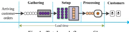
[image:3.595.57.281.236.292.2]Fig. 1 shows the work flow of the proposed uncertain MTO manufacturing environment. It illustrates one type of product being processed at a single machine station. Individual customer orders arrive at the gathering stage one by one, where once Q units of orders gather together, these batches of orders leave this stage and go into the setup stage for further work. Afterwards, these partially completed orders are moved to the processing stage to undergo further processing service on an individual basis to be converted into finished goods for immediate delivery to customers, without having to wait until the whole batch is completed.
Fig. 1. Total work flow profile
We use the term “stochastic” or “uncertain” to denote that the interarrival time of individual orders, the setup time, and the processing time are all random variables, that is, they cannot be predicted with certainty. As stated in the previous section, in order to improve the generality and exactness of the proposed model, we make no theoretical assumptions on all random variables involved. Instead, each random event is characterized by its own statistic merits, composed of its expected value (or rate) and standard deviation. This treatment can help overcome the adverse impingements of impractical assumptions on optimisation solutions.
All stages involved in the afore-mentioned manufacturing environment are assumed to be mutually independent. In the event of competition for capacitated resources, orders are served in accordance with the first-come-first-served queuing principle. Without loss of generality, we further assume that each individual order contains only one product item, and that the manufacturer is a price taker in either the perfect or the monopolistic competition environment.
The proposed model incorporates some real industrial practices. In manufacturing of specialised bicycles, for example, orders for bicycles arrive on an individual basis and are gathered by the sales department, and then some operations, such as electroplating, are conducted on a batch basis. Subsequently, a setup procedure is triggered contingent on the type of bicycle to be produced. Finally, components are assembled into finished bicycles one by one for delivery to customers. Another typical example is in the heat treatment industry, where steel alloy components arrive individually at furnaces for heat treatment. As soon as a given number of steel alloy components are batched, they are loaded as a whole for heat treatment. Subsequently, they are sandblasted on an individual basis before delivery.
B. Manufacturing Formulation
As stated previously, lead time optimisation has been one
of the critical mainstreams in operation management. Based on Fig. 1, in our research, lead time is defined as the time that elapses after an order arrives and before being delivered, as follows:
( ) ( qc) ( c) ( qs) ( s) ( qp) ( p)
E W E W E W E W E W E W E W (1) with all involved parameters defined in Table I.
According to the pioneering research works [30, 31], we have
( c) ( 1) (2 )
E W Q (2)
2 2 2
2 2
( ) , ,
2 1
bb ba bs
qs bb ba bs ba bb
c c
E W g c c
(3)
with a traffic intensity bb ( Q) (Q) and,
2
2
2 2
2
2
2 2 2
2 1 1
exp , 1
3 ( )
1 1
exp , 1
(1 )( 10 )
bb ba
ba bb ba bs
bb ba
ba bb ba bs
c
c
c c
g
c
c
c c
(4)
In the gathering stage, orders enter for being gathered in batches without queuing. Once placed, they can immediately go into this stage without any delay, thus,
( qc) 0
E W (5)
In addition, based on the probability theory, we can readily figure out:
( s) ( )
E W E T (6)
1 ( p) ( i)
E W E X
(7)
Given i (1 i Q), representing the relative position of an order in a given batch, the expected time spent in waiting for processing service by it is:
1 2 1
( qp| ) ( ... i | ) ( 1)
E W i E X X X i i (8)
Thus, the expected queuing time for processing all customer orders should be:
|
1
1 1 1 1 1
( ) ( ( )) ( ) ( 1)
2
Q qp qp i
i
i i Q
E W E E W E E i
Q
(9)Hence, Eq. (1) can be rewritten as follows:
2 2 2
2 2
1 1 1
( ) , ,
2 2 1 2
bb ba bs
bb ba bs ba bb
c c
Q Q
E W g c c
(10)
C. Commodity Pricing
As mentioned previously, scholars have suggested a negative relationship between commodity prices and lead times. Here we further illustrate this point from the perspective of the macroeconomic theory.
As illustrated in Fig. 2, the supply and the demand firstly balance at point A, where the manufacturer produces a quantity Q1 of products and sells them at the priceP1. The
decreasing lead time produces an increased market demand for the products, and therefore the demand curve shifts upward from D1 to D2. Then, a new balance between supply and demand sets up at point B. If there is no constraint on capacity, the manufacturer would choose to produce Q2 and
IAENG International Journal of Applied Mathematics, 44:2, IJAM_44_2_07
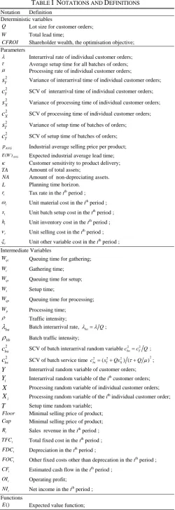
TABLE I NOTATIONS AND DEFINITIONS Notation Definition
Deterministic variables
Q Lot size for customer orders; W Total lead time;
CFROI Shareholder wealth, the optimisation objective; Parameters
Interarrival rate of individual customer orders; Average setup time for all batches of orders; Processing rate of individual customer orders;
2
Y
s Variance of interarrival time of individual customer orders;
2
Y
c SCV of interarrival time of individual customer orders;
2
X
s Variance of processing time of individual customer orders;
2
X
c SCV of processing time of individual customer orders;
2
T
s Variance of setup time of batches of orders;
2
T
c SCV of setup time of batches of orders;
AVG
p Industrial average selling price per product;
( )AVG
E W Expected industrial average lead time; Customer sensitivity to product delivery;
TA Amount of total assets;
NA Amount of non-depreciating assets.
L Planning time horizon.
t
r Tax rate in the tth period ;
t
Unit material cost in the tth period ;
t
s Unit batch setup cost in the tth period ;
t
h Unit inventory cost in the tth period ;
t
Unit selling cost in the tth period ;
t
Unit other variable cost in the tth period ; Intermediate Variables
qc
W Queuing time for gathering;
c
W Gathering time;
qs
W Queuing time for setup;
s
W Setup time;
qp
W Queuing time for processing;
p
W Processing time; Traffic intensity;
ba
Batch interarrival rate, baQ;
bb
Batch traffic intensity;
2
ba
c SCV of batch interarrival random variable 2 2
ba Y
c c Q;
2
bs
c SCV of batch service time 2 2 2 2
( ) ( )
bs T X
c s Qs Q ;
Y Interarrival random variable of customer orders;
i
Y Interarrival random variable of the ith customer orders;
X Processing random variable of individual customer orders;
i
X Processing random variable of the ith individual customer order;
T Setup time random variable; Floor Minimal selling price of product; Cap Minimal selling price of product;
t
R Sales revenue in the tth period ;
t
TFC Total fixed cost in the tth period ;
t
FDC Depreciation in the tth period ;
t
FOC Other fixed costs other than deprecation in the tth period ;
t
CF Estimated cash flow in the tth period ;
t
OI Operating profit;
t
NI Net income in the tth period ;
Functions ()
E Expected value function;
sells them at the sales prices of P2 to take all potential profits.
Subject to the capacity constraint, however, it has no extra capability to produce more products thanQ1.Consequently, it
[image:4.595.46.297.53.782.2]can only make use of this competitive advantage by asking for a price, as high as possible. Eventually, the real new balance builds at pointC, rather thanB. Thus, a decrease in lead time directly gives rise to a corresponding linear increase in sales price, and vice versa.
[image:4.595.346.509.173.300.2]Fig. 2 Supply-demand curve analysis for commodity pricing
Fig. 3 Supply-demand curve analysis for longer lead times Conversely, when the lead time becomes longer, for example, due to the machine aging or inefficient management, the manufacturer has to cut down its sales price in order to sell out all of its products to alleviate the adverse impingements arising from lengthening in lead times, as illustrated by the point E in Fig. 3. That is, an increase in lead time causes a linear decrease in sales price.
Based on the above supply-demand curve analysis and suggestions from pioneering studies [26, 27, 29], we derive a negatively linear relationship between sales prices and the expected lead time:
( ) ( )AVG AVG
p E W E W p Floor p Cap (11)
The parameter indicates the level of customer sensitivity to the delivery, and hence the lead time spread, of a product. A large means that customers are knowledgeable of the market information and have a strong desire to acquire the product soon. It is difficult to determine
theoretically for a firm because of various complicated factors. Nevertheless, it can be heuristically set between the range of 0 and 100.
IAENG International Journal of Applied Mathematics, 44:2, IJAM_44_2_07
[image:4.595.348.511.341.477.2]D. Shareholder Wealth Derivation
Firstly, the operating income can be estimated as the revenue minus the total cost of goods sold (COGS), as in
1 1 1 1 1
( )
t t t t t
DA
OI p FOC s E W h
Y L Y Y Q Y
(12)
where p1
Y represents sales revenue, and DA
L denotes the
depreciation expense when using the straight-line depreciation method; vt1
Y , 1 1
t
s
Y Q, and 1 ( ) t
E W h
Y respectively
mean the total purchasing cost, setup cost, and inventory cost. Thus,
1 1 1 1 1 1
( )
t t t t t t t t
TVC s E W h v OI r
Y Y Q Y Y Y
(13)
Finally, the period cash flow can be estimated as the net income plus noncash expenses [32], as in:
t t t t
DA
CF R TVC TFC
L
(14)
Subsequently, we have to relate these parameters for maximising the shareholder wealth in terms of CFROI. As stated previously, CFROI is a real, cross-sectional internal IRR calculated at a time point from aggregate data for a firm. It is one of economic performance metrics, focusing on the real rate of return earned on the entire assets. The basic valuation of CFROI is based on DCF. So the conception of IRR and DCF can be applied to calculate the CFROI [32], as follows:
1(1 ) (1 )
L j
j L
j
CF NA
TA
CFROI CFROI
(15)with the following constraint conditions
1 100% Q
F p C
(16)
III. NUMERICAL EXPERIMENTS
Three numerical experiments are performed to validate our proposed model. The first one compares the shareholder wealth maximisation model to the traditional operation optimisation. The second one explores the impacts of the unrealistic statistical distributions on shareholder wealth. In the last one, we test the hedging capability of our model to provide insights into how possible and at what level these risks affect the long-term sustainable interests of investors, especially equity holders.
A. Comparison of Optimisation Objectives
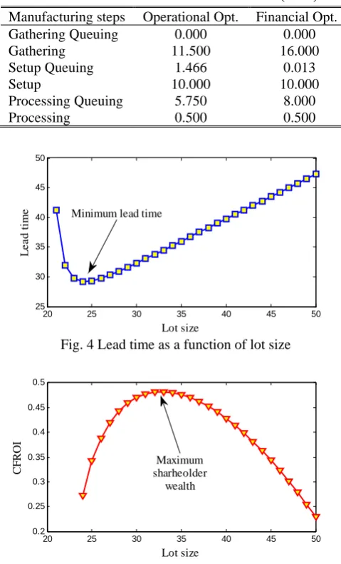
In order to better examine the difference between operational and financial optimisations, we firstly determine the optimal lot size that can minimise the total lead time, with expected times of each manufacturing step shown in Table II. Based on Eq.(10), the trend of the expected total lead time in relation to the lot size is illustrated in Fig. 4. The optimal lot size of 24 gives a minimum total lead time of 29.216 minutes with a traffic intensity of 91.67%.
TABLE II EXPECTED TIMES FOR EACH STEP (MINS)
Manufacturing steps Operational Opt. Financial Opt.
Gathering Queuing 0.000 0.000
Gathering 11.500 16.000
Setup Queuing 1.466 0.013
Setup 10.000 10.000
Processing Queuing 5.750 8.000
Processing 0.500 0.500
20 25 30 35 40 45 50
25 30 35 40 45 50
Lot size
L
ead t
im
e Minimum lead time
Fig. 4 Lead time as a function of lot size
20 25 30 35 40 45 50
0.2 0.25 0.3 0.35 0.4 0.45 0.5
Lot size
CF
ROI Maximum
sharheolder wealth
Fig. 5 Shareholder wealth as a function of lot size Then, we need to optimise our model to maximise the shareholder wealth. The resulting lot size is 33 with a CFROI value of 48.18% and a total lead time of 34.513. Fig. 5 shows the effect of various lot sizes on the CFROI metric as the lot size increases, while Table II provides more details on the expected times for each manufacturing procedure and corresponding queuing delay.
It can be seen that the expected collecting time increases by about 39.13%, from 11.500 minutes to 16.000 minutes, while the expected queuing time for the processing service jumps from 5.750 minutes to 8.000 minutes. Conversely, the expected queuing time for the setup service drops drastically by 99.12%, from 1.466 minutes to 0.013 minutes. To a great extent, the decrease of time spent in the setup service offsets the time increase in the gathering service and processing delay. In comparison with the lead time optimisation, the total lead time increases only slightly under the financial optimisation when the fixed lot size changes from 24 to 33.
B. Shareholder Wealth under Theoretical Assumptions
Here we consider a theoretical case to validate the extensibility of our proposed model. Several theoretical assumptions will be made. Interarrival of orders follows a
IAENG International Journal of Applied Mathematics, 44:2, IJAM_44_2_07
[image:5.595.303.543.60.456.2]Poisson process, while the processing time is exponentially distributed. We also assume that the setup time is completely deterministic, such that 2
ba
c Q and 2 2
bs
c Q Q .
Hence, Eq.(10) can be reorganized by substituting these new expressions for the older ones, as follows:
1 1 1
( ) ( )
2 qs 2
Q Q
E W E W
(17)
where,
2 2
2
2 2
( )
( )
2 ( )
2 ( ) ( ) ( )
exp
3 ( )
qs
Q Q
E W
Q Q Q
Q Q Q Q
Q Q Q
(18)
20 25 30 35 40 45 50
25 30 35 40 45 50
Lot size
Le
a
d
t
im
[image:6.595.51.289.95.369.2]e Minimum lead time
Fig. 6 Lead time as a function of lot size under theoretical assumptions
20 25 30 35 40 45 50
0.2 0.25 0.3 0.35 0.4 0.45 0.5
Lot size
CF
R
O
I
Maximum shareholder
[image:6.595.306.549.202.287.2]wealth
Fig. 7 CFROI as a function of lot size under the theoretical assumptions
Next, we need to recalculate the optimal lot sizes under the theoretical case. Fig. 6 shows the relation between the lot size and the lead time under the above assumptions. The minimum total lead time of 29.938 corresponds to the lot size of 25 with a traffic intensity of 90.00%. The time consumptions for each manufacturing step are given in Table III. Here the shareholder value optimisation leads to an optimal lot size of 33 with a maximum CFROI value of 47.93%. Fig. 7 illustrates the effects of various lot sizes on the shareholder wealth, while Table III shows the time consumptions for each service.
It can be seen that the time consumed on gathering increases from 12.000 to 16.500 minutes, approximately an increase of 37.50%. In the processing stage, more 2.250 minutes are spent in the processing service. Queuing time for setup service drops from 1.438 to 0.041 minutes. Similarly, mutual offset of these manufacturing times only lead to a
slight increase of the total lead time, from 29.938 up to 34.559, under the theoretical case when the optimal lot size changes from 25 to 33.
It is worth noting that the shareholder wealth decreases from 48.18% without statistical assumptions on random variables to 47.93% under the theoretical assumptions. This further demonstrates that incorrect distributions assumptions are always unrealistic and misleading.
TABLE IIIEXPECTED TIMES FOR EACH MANUFACTURING STEP UNDER THE THEORETICAL ASSUMPTIONS (MINS) Manufacturing steps Operational Opt. Financial Opt. Gathering Queuing 0.000 0.000
Gathering 12.000 16.500
Setup Queuing 1.438 0.041
Setup 10.000 10.000
Processing Queuing 6.000 8.250
Processing 0.500 0.500
C. Sensitivity Analysis
Finally, we take a closer look at how sensitive the shareholder wealth is to two key parameters and st .
We firstly examine the effects of customer sensitivity levels to lead time,, on the shareholder wealth. Table IV lists the optimal CFROI values and corresponding lead times as deceases from 100 to 0. The lower its value, the more indifferent the customers are to the changes in lot sizes and lead times. Fig. 8 shows the curves of the lead time and the CFROI metric for a various range ofvalues. The figure illustrates that different values have no effects on the curve shape of the lead time, but it distorts the curve shape of the shareholder wealth.
Table IV and Fig. 8 have two important implications. The first is that the optimisation results under both the operational and financial cases are much closer when the value is large enough. Second, the proposed model has almost the same optimisation result regardless of the value when it is small enough.
The second implication can be directly reflected in (11). When the value is small enough, E W( )E W( )AVG is
nearly zero and can be ignored. In other words, the selling price approximately equals pAVG . Thus, in this case, the changes of almost have no effect on the shareholder wealth, as illustrated in Table IV and Fig. 8.
TABLE IVEFFECTS OF CUSTOMER SENSITIVITY TO LEAD TIME ON SHAREHOLDER WEALTH
Lot Size CFROI Lead Time (mins)
100 25 360.46% 29.938
10 28 73.60% 31.148
1 32 49.91% 33.835
0.1 33 48.11% 34.559
0 33 47.91% 34.559
IAENG International Journal of Applied Mathematics, 44:2, IJAM_44_2_07
[image:6.595.59.284.391.531.2] [image:6.595.308.544.695.769.2]20 30 40 50 -50
-40 -30 -20
Lot Size
N
e
g
a
tiv
e
L
e
a
d
Ti
m
e
20 30 40 50
0 5
Lot Size (k=100)
CF
RO
I
20 30 40 50
1 2
Lot Size (k=10)
CF
RO
I
20 30 40 50
1 1.5 2
Lot Size (k=1)
CF
RO
I
20 30 40 50
1 1.5
Lot Size (k=0.1)
CF
RO
I
20 30 40 50
1 1.5
Lot Size (k=0)
CF
RO
[image:7.595.54.275.57.237.2]I
Fig. 8 Lead time and shareholder wealth against lot sizes under various customer sensitivities
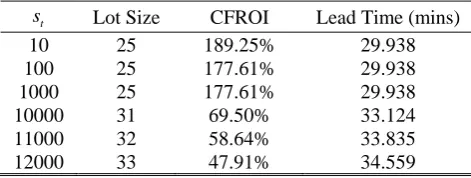
Another concern is how the setup cost can affect the shareholder wealth. Table V lists the optimal fixed lot sizes, the corresponding CFROI values and lead times for a various series of setup costs. This table shows that when setup costs are low enough, the financial optimisation results in the similar optimal lot sizes to the operational model. For example, when St10, the optimal fixed lot size in the first
numerical experiment is 24, while the resulting optimal lot size is 25 under the financial optimisation. However, as soon as the setup cost increases to a certain degree, its impact on the shareholder wealth becomes more substantial.
TABLE VEFFECTS OF SETUP COST ON SHAREHOLDER WEALTH
t
s Lot Size CFROI Lead Time (mins)
10 25 189.25% 29.938
100 25 177.61% 29.938
1000 25 177.61% 29.938
10000 31 69.50% 33.124
11000 32 58.64% 33.835
12000 33 47.91% 34.559
IV. CONCLUSION
This paper attempts to address the infeasibility issues in traditional manufacturing optimisation based on operational objectives. It proposes a stochastic lot-sizing optimisation model for make-to-order manufacturing to maximise a financial objective. The proposed model incorporates financial and economic parameters relevant for a firm’s business goal of maximising the shareholder wealth, measured by CFROI. It assumes individual arrivals and departures and general distribution of random variables. This treatment enables the proposed model to deal with relatively more realistic demand patterns, and enhances its generality and extensibility.
Numerical experiments show that when the setup costs are low and the customer sensitivity to lead time is high, there is no significant difference between operational optimisation
and financial optimisation. However, if the setup costs are high or the customer sensitivity to lead time is low, the optimal lot size for operational optimisation is generally much smaller than for maximisation of the shareholder wealth. This validates that traditional operational optimisation is not necessarily in line with the overall business goal of a firm, and thus highlights the importance of considering financial and economic parameters for optimising manufacturing decisions.
A limitation of the proposed model is that it focuses only on a single-item, single-machine stochastic lot-sizing scenario. It would therefore be worthwhile to extend it for dealing with relatively more complicated manufacturing environments. Moreover, further research work would be needed to examine the relationship between the lead time spread and the selling prices.
REFERENCES
[1] Karmarka, U.S., Kekre, S., Kekre, S. and Freeman, S., Lot-sizing and Lead-time Performance in a Manufacturing Cell. INTERFACE, 1985.
15(2): pp. 1-9.
[2] Buzacott, J.A. and R.Q.Zhang, Inventory management with asset-based fianncing. Managment Science, 2004. 50(9): pp. 1274-1292.
[3] Lambrecht, M.R., Chen, S. and Vandaele, N.J., A lot sizing model with queueing delays: The issue of safety time. European Journal of Operational Research, 1996. 89(2): pp. 269-276.
[4] Bertrand, J.W.M., Multiproduct Optimal Batch Sizes with In-Process Inventories and Multi Work Centers. IIE Transactions, 1985. 17(2): pp. 157-163.
[5] Choi, S. and Enns, S.T., Multi-product capacity-constrained lot sizing with economic objectives. International Journal of Production Economics, 2004. 91(1): pp. 47-62.
[6] Madden, B.J., CFROI Valuation: A Total System Approach to Valuing the Firm. 2002, Oxford: Butterworth Heinemann.
[7] Erasmus, P.D. and Lambrechts, I.J., EVA and CFROI: A comparative analysis. Management Dynamics, 2006. 15(1): pp. 14-26.
[8] Young, S.D. and O'Byrne, S.F., EVA and Value-Based Managment: A Practical Guide to Implementation. 2001, USA: McGraw-Hill. [9] Karmarkar, Lot sizes, manufacturing lead times and Utilization, in
Graduate School of Management, Working Paper No.QM8314, University of Rochester, Rochester, New York1983.
[10] Dobson, G., Karmarkar, U.S. and Rummel, J.L., Batching to Minimize Flow Times on One Machine. Management Science, 1987. 33(6): pp. 784-799.
[11] Govil, M.K. and Fu, M.C., Queueing theory in manufacturing: A survey Journal of Manufacturing Systems, 1999. 18(3): pp. 214-240. [12] Tielemans, P.F.J. and Kuik, R., An exploration of models that minimize
leadtime through batching of arrived orders. European Journal of Operational Research, 1996. 95(2): pp. 374-389.
[13] Erasmus, P.D. and Lambrechts, I.J., EVA and CFROI: A comparative analysis. Ma Dynam, 2006. 15(1): pp. 14-26.
[14] Wang, X.J. and Choi, S.H. Lot Sizing Optimisation for Stochastic Make-to-order Manufacturing, Lecture Notes in Engineering and Computer Science: Proceedings of The International MultiConference of Engineers and Computer Scientists 2014, IMECS 2014, 12-14 March, 2014, Hong Kong, pp. 938-943.
[15] Wang, X.J. and Choi, S.H. Stochastic multi-item lot sizing for the shareholder wealth maximisation, Lecture Notes in Engineering and Computer Science: The World Congress on Engineering 2013, WCE 2013, 3-5 July, 2013, London, UK, pp. 420-425.
[16] Wang, X.J. and Choi, S.H., Optimisation of Stochastic Multi-item Manufacturing for Shareholder Wealth Maximisation. Engineering Letters, 2013. 21(3): pp. 127-136.
[17] Lazonick, W. and O'Sullivan, M., Maximizing shareholder value: a new ideology for corporate governance. Economy and Society, 2000.
29(1): pp. 13-35.
[18] Johnson, T. and Kaplan, R., Relevance lost: The rise and fall of management accounting. 1987, Boston: Harward Business School Press.
IAENG International Journal of Applied Mathematics, 44:2, IJAM_44_2_07
[image:7.595.50.286.462.551.2][19] Morse, W., Davis, J. and Hartgraves, A., Management accounting: A strategic approach. 1996, Cincinnati: Southwestern Publishing. [20] Kramer, J.K. and Peters, J.R., An interindustry analysis of Economic
Value Added as a proxy for Market Value Added. Journal of Applied Finance, 2001. 11(1): pp. 41-49.
[21] De Villiers, J.U., The distortions in Economic Value Added (EVA) caused by inflation. Journal of Economics and Business, 1997. 49: pp. 285-300.
[22] Farsio, F., Degel, J. and Degner, J., Economic Value Added (EVA) and Stock Returns. The Financier, 2000. 7(1-4): pp. 115-118.
[23] Madden, B.J., CFROI Valuation: A Total System Approach to Valuing the Firm. Vol. 5-6. 2002, Oxford: Butterworth Heinemann.
[24] Martin, J.D. and Petty, J.W., Value Based Management: The Corporate Response to teh Shareholder Revolution. 2000, New York: Oxford University Press.
[25] Obrycki, D.J. and Resendes, R., Economic Margin: The Link Between EVA and CFROI. 2000, New York: John Wiley and Sons.
[26] So, K.C. and Song, J.S., Price, delivery time guarantees and capacity selection. European Journal of Operational Research, 1998. 111(1): pp. 28-49.
[27] Weng, Z.K., Manufacturing lead times, system utilization rates and lead-time-related demand. European Journal of Operational Research 1996. 89(2): pp. 223-444.
[28] Kenyon, G.N., A profit-based lot-sizing model for the n-job,m-machine job shop Incorporating quality, capacity, and cycle time, 1997, Texas Tech University: Texas.
[29] George, K., Canel, C. and Neureuther, B.D., The impact of lot-sizing on net profits and cycle times in the n-job, m-machine job shop with both discrete and batch processing. International Journal of Computer Integrated Manufacturing, 2005. 97(3): pp. 263-278.
[30] Lambrecht, M.R. and Vandaele, N.J., A general approximation for the single product lot sizing model with queueing delays. European Journal of Operational Research, 1996. 95(1): pp. 73-88.
[31] Whitt, W., The Queueing Network Analyzer. The Bell System Technical Journal, 1983. 62(9): pp. 2779-2815.
[32] Bodie, Z., Merton, R.C. and Cleeton, D.L., Financial Economics. 2 ed2008, USA: Pearson Prentice Hall.