Abstract—Multistage stochastic programs are effective for solving long-term planning problems under uncertainty. Such programs are usually based on scenario generation model about future environment developments. In the present paper, the scenario model is developed for the case when enough data paths can be generated, but due to solvability of stochastic program the scenario tree has to be constructed. The proposed strategy is to generate multistage scenario tree from the set of individual scenarios by bundling scenarios based on cluster analysis. The K-means clustering approach is modified to capture the interstage dependencies. Such generation of scenario tree can be useful in cases when it is difficult to construct the adequate scenario tree from the stochastic differential equations or time-series models, and the sampled paths can be obtained by sampling or resampling techniques. While generating the initial fan of individual scenarios, the copula is employed for modeling the dependence between stochastic variables in a multivariate structure. It allows to model nonlinear dependencies between non-elliptically distributed stochastic variables. While investigating the copula effect on the scenario tree structure, we will try to answer the question: does the copula features are captured in the approximate representation of uncertainty in the form of scenario tree. The proposed scenario tree generation method is implemented on sampled data of discount bond yields. The Gaussian copula and Student’s t-copula are employed while generating the set of individual scenarios in the multivariate structure.
Index Terms—Copula, K-means clustering, Multistage scenario tree construction, Stochastic programming.
I. INTRODUCTION
The concept of scenarios is usually employed for the modeling of randomness in stochastic programming models [1], [2], in which data evolve over time and decisions have to be made independently upon knowing the actual paths that will occur. Such data are usually subject to uncertainty or some kind of risk. For instance, the random variables are the return values of each asset on an investment in portfolio management problems, and the investment decisions must be implemented before the asset performance can be observed. Each scenario can be viewed as one realization of an underlying multivariate stochastic data process. The modeling of randomness
Manuscript received October 03, 2007.
K. Sutiene is with the Business Informatics Department, Kaunas University of Technology, Studentu 56-301, Kaunas LT-51424, Lithuania (corresponding author to provide phone: 370-681-52842; fax: 370-37-451654; e-mail: [email protected]).
H. Pranevicius is with the Business Informatics Department, Kaunas University of Technology, Studentu 56-301, Kaunas LT-51424, Lithuania (e-mail: [email protected]).
employees the set of available past data with the aim of building submodels for each individual stochastic parameter. These submodels are used to generate a set of scenarios that encapsulate the consistent depictions of pathways to possible futures based on assumptions about economic and technological developments. Thus, the factors driving risky events are approximated by a discrete set of scenarios, or sequence of events. This process is known as scenario generation. Scenarios can be generated using various methods, based on different principles: conditional sampling, sampling from given marginals and correlations, moment matching, path based methods, optimal discretization, as in [3]–[7]. Stochastic programming (optimization) has been applied in the following areas: 1) Manufacturing production capacity planning; 2) Electrical generation capacity planning; 3) Asset liability management; 4) Portfolio selection; 5) Traffic management; 6) Machine scheduling. In these applications decisions must often be taken in the face of the unknown.
A good approximation may involve a very large number of scenarios with probabilities. A better accuracy of uncertainties is described when scenarios are constructed via a simulated data path structure, also known as a scenario fan. But the number of scenarios is limited by the available computing power, together with a complexity of the decision model. To deal with this difficulty, we can reduce the dimension of the initial scenario set by constructing the multistage scenario tree out of it. The decision on the number of stages, on the size of time periods and on the branching scheme is very important for a good representation of the uncertainty in the form of scenario tree, which is input into the multistage stochastic program. The detailed description of both scenario fan and scenario tree will be given in Section III.
In the present paper, we concentrate on the generation of scenario trees when the underlying stochastic parameters have been determined and the data paths of their realizations can be generated. The scenario tree can be constructed out of sampled paths by employing some classifying method, such as clustering analysis. While bundling the scenarios to the clusters, the interstage dependencies have to be captured. An approach similar to our work is introduced in the article [8], but without a detailed clustering algorithm. Due to this, the K-means clustering method is modified to treat properly the interstage dependencies and is implemented while constructing the scenario tree from simulated data paths.
Such generation of scenario tree can be useful in cases when it is difficult to construct the adequate scenario tree from the stochastic differential equations or time-series models, and the sampled paths can be obtained by sampling or simulation
Copula Effect on Scenario Tree
K. Sutiene and H. Pranevicius
techniques. The proposed scenario tree construction algorithm allows incorporating a copula-based dependence measure [9], [10] to describe the dependence between stochastic variables in a multivariate structure. Due to assumptions of using the Pearson’s correlation coefficient, the usefulness of such correlation is restricted. The main advantage of employing copulas is that they allow to model the nonlinear dependencies between non-elliptically distributed stochastic variables. The copula function has been introduced in finance by Embrechts, McNeil, and Straumann [9]. To our knowledge, the copulas still are not very popular in generating the scenario trees. According to this, we propose to approximate the multivariate stochastic process by a scenario fan with multivariate structure using copulas. Then, the scenario tree is constructed out from the sampled paths using the modified K-means clustering algorithm. Numerical experience is reported for constructing multivariate scenario trees of discount bond yields, employing two separate – Gaussian and Student’s t – copulas.
The rest of the paper is organized as follows. The scenario generation model is introduced in Section II. The mathematical model consists of two main components: models for the univariate marginal distributions of uncertain factors and a model of the dependence structure employed in the notion of copulas. Gaussian copula and Student’s t-copula are considered. The simulation algorithm of modeling the copula based dependent data is given. Section III discusses how the copula function can be incorporated while generating scenarios. Section IV describes how the simulated data paths can be transformed to the scenario tree using cluster analysis. The K-means clustering algorithm is modified to bundle the time-dependent data. Section V demonstrates the numerical example of scenario tree generation based on discount bond yields data. Finally, some concluding remarks are given.
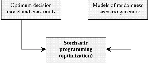
II. SCENARIO GENERATION COMPUTATIONAL PROCEDURE Stochastic programming (optimization) combines model of optimum resource allocation and models of randomness, thereby it creates a decision making framework (see Fig. 1) [11]. Whereas deterministic optimization problems are formulated with known parameters, real world problems almost invariably include parameters which are unknown at the time a decision should be taken. That’s why the deterministic
Optimum decision model and constraints
Models of randomness – scenario generator
Stochastic programming (optimization)
Fig. 1. Stochastic programming paradigm
approach is expanded.
In stochastic programs the first element is the objective function which together with the constraints describes the core of the problem that has to be solved and varies with each individual application. The second element is the scenario generator, and it is used to describe the uncontrollable (risk) factors affecting the relevant system, such as, inflation rate, interest rate, GPD – factors that are not under control of the decision makers. The uncertain elements are modeled as random variables to which the probability theory can be applied. A concept of scenarios is used to represent of how the future might unfold. Some kind of probabilistic model or simulation can be used to generate a batch of scenarios. The models of randomness with their finite and discrete realizations are called scenario generators. The outcome of such system is uncertain even when the values of all the decision variables are fixed. Scenarios can also be used in descriptive models, where a set of mathematical operations are defined that can predict how a mathematical system will behave, e.g. Markov models.
The main feature of stochastic programming is its multistage formulation. Despite rich involvement of the future, everything is aimed to make a well hedged decision in the present. The attitude is adopted that a decision will be properly made in the present only taking into account, at least some to extent, the opportunities for modification or correction at later times. Decisions at later times can respond to the information that has become available since the initial decision. Thus, during the time the decisions alternate with observations: initial decision
→ observation → recourse decision → observation → … →
recourse decision. This sequence doesn’t go on indefinitely, but the number of stages can be large enough. Decisions that are taken have no effect on the probability structure. Thus, we have a multistage problem. The number of stages is used in modeling the uncertainty; we will formalize this later in terms of the multistage scenario tree.
In the paper [11], the general scenario generation procedure for multistage stochastic programs is given. We append this procedure with additional step (Step 2), paying the important attention to the dependence modeling among risk factors. The following steps (some or all) have to be performed while generating scenarios:
1) Collecting historical data of stochastic parameters, assumptions of a model, estimation/calibration of parameters for a chosen model.
2) Choosing the appropriate model to describe the dependence structure among stochastic parameters.
3) Generation of scenarios according to the chosen model or discretization of the distributions using approximation of statistical properties.
We will consider all these steps in deeper manner.
A. Modeling Paradigm
[image:2.612.53.295.599.705.2]variables among the uncontrollable inputs. In paper [12], the author proposes four types of problems, concerning the level of the available information:
1) Full knowledge of underlying probability distribution ; 2) Known parametric family ;
3) Sample information ; 4) Low information level.
These four groups are not strictly distinguishable. Different information levels can be applied to the distinct parameters of the model. The most popular modeling paradigms are [11]:
• Econometric Models and Time Series (ARMA, GARCH, VAR models) ;
• Geometric Brownian Motion (Diffusion Processes) ;
• Artificial Intelligence (Neural Networks) ;
• Statistical Approaches (Statistical approximation, Forecasting, Moment Fitting) ;
• Sampling.
It is very important that the sample we use to represent the stochastic parameters in the form of scenarios would be consistent with empirical data. Therefore, one has to specify the stochastic processes for risk parameters, and estimate the parameters of such models using empirical data.
B. Dependence structure modeling
In this paper we concentrate on generation of scenarios representing the realizations of multivariate stochastic process whose components are correlated. We define such scenarios as intercorrelated scenarios, meaning that they correlate through the components of multivariate structure. Historically measuring and modeling of dependence has centered on correlation. The modeling of dependent variables is performed employing the Pearson’s correlation matrix to describe the multivariate structure. Many applications show that relationships among stochastic variables may be very complex, and linear dependence can’t reflect these relationships adequately. The reason is that the Pearson’s correlation
-4 -3 -2 -1 0 1 2 3 4
-4 -3 -2 -1 0 1 2 3
4 1000 Simulated Dependent Values
X1~Normal(0,1)
X
2~
N
orm
al
(0,
1)
(a) Dependence between X1 and X2 with ρ=0.7
-4 -3 -2 -1 0 1 2 3 4 -4
-3 -2 -1 0 1 2 3
4 1000 Simulated Dependent Values
X1~Normal(0,1)
X
2~
N
or
m
al
(0,
1)
[image:3.612.338.542.62.255.2](b) Dependence between X1 and X2 with ρ=0.7
Fig. 2. Different dependence structures
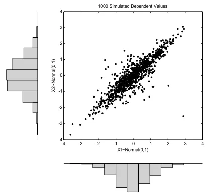
coefficient does not capture any non-linear dependencies, and it is usually used assuming the elliptical shape of normal distribution in applications. We include Fig. 2 as motivation for the ideas of this paper. It shows 1000 random variates from two distributions with identical standard Gaussian marginal distributions: case (a) and case (b) depict bivariate structure of
1
X and X2 with linear correlation coefficient ρ=0.7 . However, the dependence structure between X1 and X2 is qualitatively quite different. It relates that in case (b) extreme values have a tendency to occur together. This example shows that the dependence between random variables cannot be distinguished on the grounds of correlation alone. Additionally, in real applications it is rare for distributions to follow the strict spherical assumptions with a constant dependence across the distribution implied by correlation.
To overcome the limitations of correlation, the practitioners can draw on copula functions. It is very powerful technique, which allows to represent joint distribution by splitting the marginal behavior, embedded in the marginal distributions, from the dependence, captured by the copula itself. This superiority of using copulas releases the modeling, estimation and simulation of dependent random variables. Let define the copula itself.
A function C is the d-dimensional copula if it fulfills the following properties [13]:
1) The domain of C is
[ ]
0,1d; 2) C is grounded and d-increasing ;3) The margins Ck of C satisfy Ck
( )
u =u, k=1,2,K,dfor all u in
[ ]
0,1 .Let consider d random variables Y1,Y2,K,Yd with
multivariate distribution F and univariate margins
( ) ( )
y F y Fd( )
ydF1 1, 2 2,K, . Sklar’s theorem, which is the
foundation for copulas, states that any joint distribution can be written in a copula form.
Sklar’s Theorem (1959). Given a joint distribution function
(
y y yd)
F 1, 2,K, for random variables Y1,Y2,K,Yd with
marginals
(
F1,F2,K,Fd)
, F can be written as a function of its marginals:(
y y yd)
C(
F( ) ( )
y F y Fd( )
yd)
F 1, 2,K, = 1 1, 2 2 ,K, ,
where copula C
(
u1,u2,K,ud)
is a joint distribution withuniform marginals. Moreover, if each Fi is continuous, C is
unique.
The dependence structure can be represented by a proper copula function. Moreover, the following corollary is attained from Sklar’s theorem.
Corollary. Let F be an d - dimensional distribution function with continuous margins F1
( ) ( )
y1,F2 y2 ,K,Fd( )
yd ,and copula C. Then, for any u=
(
u1,u2,K,ud)
in[ ]
d
1 ,
0 :
(
u u ud)
F(
F( )
u F( )
u Fd( )
ud)
C 1
2 1 2 1 1 1 2
1, , , , , ,
− −
−
= K
K
where −1
i
F is the generalized inverse of Fi.
A good many copulas are available, with differing characteristics that lead to the different relationships among variables generated. Note that copulas differ not so much in the degree of association they provide, but rather in which part of the distributions the association is strongest: the behavior of copulas in the right and left tails can be used to distinguish among joint distributions that produce the same overall correlation.
In this paper, we will consider two copulas: Gaussian copula and Student’s t-copula. These copulas do not have a simple closed form, but are implied by well known multivariate distribution functions: multivariate Gaussian and multivariate Student’s t distributions respectively. The difference between these two copulas is that the Student’s t-dependence structure supports joint extreme movements regardless of the marginal behavior of stochastic variable compared with the Gaussian copula. A complete copula-based joint distribution can be constructed using assessed rank-order correlations and marginal distributions. Examples of rank-order correlations are Spearman’s rho and Kendall’s tau correlations, which are used to describe the dependence relations of a monotonic nature: it indicates the tendency of two random variables to increase/decrease concomitantly (positive dependence) or contrariwise (negative dependence).
The Gaussian or normal d-copula is given by
( )
dCor(
( )
( )
( )
d)
GaCor u u u u
C 1
2 1 1
1 , − , , −
− Φ Φ
Φ Φ
= K ,
where Φ denotes the standard univariate normal distribution function and d
Cor
Φ denotes the standard multivariate normal
distribution function with matrix Cor of linear correlation coefficients. The main property of such dependence structure is that Gaussian copula does not have neither upper nor lower tail dependence.
Simulation procedure for Gaussian copula is performed as follows:
(a) convert Kendall’s tau corijτ to the linear correlation
coefficient corij using formula corij =sin
(
πcorijτ /2)
(therelationship between the linear correlation coefficient corij
and Spearman’s rho S ij
cor is 2sin
(
S/6)
ijij cor
cor = π ) and
construct the lower triangular matrix Α=
[ ]
aij that holdsA A Cor= ′ ;
(b) generate independent standard normal variables εi ,
d
i=1, and form a column vector ε ;
(c) construct a joint probability density function, taking the matrix product ε~=Aε ;
(d) set u~i =Φ
( )
ε~i ;(e) set x~i
( )
u~i1
−
Φ
= .
At the result, x~ , i i=1,d are dependent variables based on
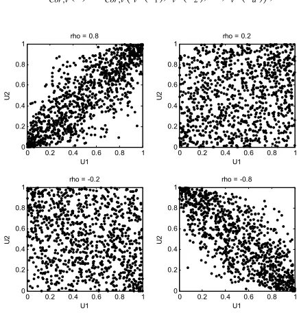
Gaussian copula. Fig. 3 shows four scatter plots of 1000 random values from a bivariate Gaussian copula for various levels of correlation coefficient to illustrate the range of different dependence structures. Thus, the family of Gaussian copulas is parameterized by the linear correlation matrix.
The Student’s t-dependence structure introduces an additional parameter compared with the Gaussian copula, namely the degrees of freedom. Student’s t-copula can be written as
( ) ( )
( )
(
v v v d)
d v Cor t
v
Cor u t t u t u t u
C 1
2 1 1 1 ,
, ( ) , , ,
~ = − − −
K ,
0 0.2 0.4 0.6 0.8 1 0
0.2 0.4 0.6 0.8
1 rho = 0.8
U1
U2
0 0.2 0.4 0.6 0.8 1 0
0.2 0.4 0.6 0.8
1 rho = 0.2
U1
U2
0 0.2 0.4 0.6 0.8 1 0
0.2 0.4 0.6 0.8 1
rho = -0.2
U1
U2
0 0.2 0.4 0.6 0.8 1 0
0.2 0.4 0.6 0.8 1
rho = -0.8
U1
[image:4.612.326.544.473.701.2]U2
where Cor, are the parameters of t-copula, v d v Cor
t , denotes the joint distribution function of the d -variate Student’s t-distribution with v degrees of freedom, −1
v
t is the inverse of univariate Student’s t-distribution with v degrees of freedom. Student’s t-copula has the additional parameter v comparing with Gaussian copula. Increasing the value of v decreases the tendency to discover extreme co-movements.
Simulation procedure for Student’s t-copula is performed as follows:
(a) convert Kendall’s tau corijτ to the linear correlation
coefficient corij using formula corij =sin
(
πcorijτ /2)
(therelationship between the linear correlation coefficient corij
and Spearman’s rho S ij
cor is 2sin
(
S/6)
ij
ij cor
cor = π ) and
construct the lower triangular matrix Α=
[ ]
aij that holdsA A Cor= ′ ;
(b) generate independent standard normal variables εi ,
d
i=1, and form a column vector ε ;
(c) construct a joint probability density function, taking the matrix product ε~= Aε ;
(d) generate a random variate ~ 2
v
χ
γ ;
(e) calculate ε~~= vε~ γ ; (f) u~~i=tv
( )
ε~~i ;(g) x~~i=Φ−1
( )
u~~i .At the result, ~~xi are dependent variables based on Student’s
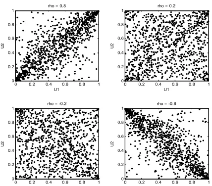
t-copula. Fig. 4 shows four scatter plots of 1000 random values from a bivariate Student’s t-copula, with degrees of freedom equal 2, for various levels of correlation coefficient to illustrate the range of different dependence structures. These plots demonstrate that t2-copula differs from Gaussian copula (see Fig. 3), even when their components have the same correlation.
0 0.2 0.4 0.6 0.8 1
0 0.2 0.4 0.6 0.8
1 rho = 0.8
U1
U2
0 0.2 0.4 0.6 0.8 1
0 0.2 0.4 0.6 0.8
1 rho = 0.2
U1
U2
0 0.2 0.4 0.6 0.8 1
0 0.2 0.4 0.6 0.8
1 rho = -0.2
U1
U2
0 0.2 0.4 0.6 0.8 1
0 0.2 0.4 0.6 0.8
1 rho = -0.8
U1
U2
Fig. 4. Student’s t dependence structures with degrees of freedom equal 2, but different correlation coefficients
0 10
20 30
40 -1
0
1 0
0.2 0.4 0.6 0.8 1
Correlation coefficient Student's t-copula tail effect
[image:5.612.342.561.51.220.2]Degrees of freedom
Fig. 5. Tail dependence for t2-copula
The main difference between the considered copula functions is in measuring the dependence between the occurrences of extreme values. Bivariate tail dependence coefficient measures the strength of dependence in the upper and lower quadrant tail of a bivariate distribution. The upper tail dependence coefficient is as follows [10]:
(
)
(
( )
α( )
α)
λ
α
1 1 1 1 2 2 1 2
1, lim
− −
→ > >
= PY F Y F
Y Y
U .
Analogously, the lower tail dependence coefficient is
(
)
(
( )
α( )
α)
λ
α
1 1 1 1 2 2 0 2
1, lim
− −
→ ≤ ≤
= PY F Y F
Y Y
L .
The upper (lower) coefficient quantifies the probability to observe a large (small) Y2 , when Y1 is large (small). If
(
0,1]
, L∈ U λ
λ , then two random variables Y1 and Y2 are said to be asymptotically dependent in tails. And if λU =0,λL=0, then variables are said to be asymptotically independent in tails. Furthermore, given the radial symmetry property of elliptical distributions, the lower and upper tail dependence coefficients coincide. In the work [10], it was shown that tail dependence coefficient is equal to zero, confirming the asymptotic independence in tails of the Gaussian copula. Student’s t-copula tail effect from both degrees of freedom and correlation coefficient is depicted in Fig. 5. One can see that the stronger the linear correlation coefficient and the lower the degrees of freedom, the stronger is tail dependence.
Calibrating the copula parameters to the real data is the active research area in the current statistics literature [10, 14, 15, 16]. Most popular approaches used in estimation of copula are Exact Maximum Likelihood method (EML), Inference Functions for Margins method (IFM), Canonical Maximum Likelihood method (CML) and others. In this work, we won’t go into the details of parameterizing the copula.
During the discretization process of d-dimensional distribution function F, one can strengthen the dependence in different parts of distribution through the choice of copula.
[image:5.612.64.278.521.709.2]Indeed, the assumption of normality for the margins can be removed and
(
F1,F2,K,Fd)
may be fat-tailed distributions(e.g. Student, Weibull, Pareto), and dependence may be characterized by a Normal or other chosen copula. That is, the dependence structure between stochastic variables can be modeled independently of marginal distributions.
C. Generation of Scenarios
The four main scenario generation approaches are [3]: 1) Sampling. Sampling approaches are Monte Carlo
(Random) Sampling, Importance Sampling, Bootstrap Sampling, and Conditional Sampling. For each sampling method, the main principle is to take a sample from a probability distribution function so that for a given value we have an associated probability, which gives the scenario value and its branch probability.
2) Statistical Approaches. The main principal is to determine the value of particular statistical properties of given data. The most popular is statistical moment or property matching approach, whereby we do not assume knowledge of a random variable’s probability distribution function. Instead we describe the distribution by its statistical moments or other properties, e.g. mean, variance, percentile.
3) Simulation. It is an approach for scenario generation, where some underlying mathematical process is simulated: random numbers are incorporated into the random component of an equation and the result is recorded. Scenario generation by simulation results the set of simulated data paths with equal probability. To reduce the number of paths sometimes paths are bounded by some method. Stochastic Process Simulation, Error Correction Model, Vector Autoregressive model are most popular simulations used for stochastic programming.
4) Other methods. It can be methods from other fields, such as Artificial Neural Networks, Clustering, or it can be combination of some scenario generation methods.
None method of scenario generation is approved as optimal but the goal should be the adequate representation of uncertainty.
To remember the idea of this paper, we aim to incorporate a copula in generation of scenarios. In the paper [17], the moment matching method was used to generate copula based correlated scenarios. In our paper, we will use the combination of some methods allowing us to employ copula functions for modeling dependent stochastic variables: the simulation and clustering approaches are combined to construct the scenario tree. In the next section the stochastic programming notation is given to make the description of scenario generation more formal.
III. STOCHASTIC PROGRAMMING NOTATION
In multistage stochastic programs the underlying multivariate stochastic data process has to be discrete in time. Mathematically, we have a time index t=
{
0,K,T}
and a timehorizon consisting of T stages. The stochastic process
{ }
T t t =1= ξ
ξ is defined on some filtered probability space
(
Ω,S,F,P)
. The sample space Ω is defined asT Ω × Ω × Ω =
Ω: 1 2 K , where d
t ⊂R
Ω . Note that the sample spaces are taken as finite dimensional. In this case, we consider
d-dimensional spaces, but in other applications it is possible to vary the dimensionality. For instance, these data may correspond to the observed return of d financial assets at different time moments t. The σ -algebra S is the set of events with assigned probabilities by measure P, and
{ }
Ft Tt=1 is a filtration on S. The decisions are of two types: the initial decision x0 taken at initial time moment and the recourse decisions xt , t>0 taken at T recourse stages. Thus, thedecision at stage t is the random variable : nt;
t
x Ω→R
decisions are set as finite dimensional, but of possibly varying dimensionality. In the stochastic programming model the observations and decisions are given as a sequence
(
x) (
x) (
T xT)
x0, ξ1, 1, ξ2, 2 ,K,ξ , , where
{ }
T t t
x
x= =0 is a decision process, measurable function of ξ . The constraints on a decision at each stage involve past observations and decisions. It means that decision xt at t is measurable with respect to
F
Ft⊆ . Thus, following [8] the decision process is said to be nonanticipative. It means that the decision xt =xt
(
xt−1,ξt−1)
taken at any t>1 does not directly depend on future realizations of stochastic parameters or on future decisions. At the time when initial decision must be chosen, nothing about the random elements in our process has been pinpointed. But in making a recourse decision we have the revealed current information until this moment and the residual uncertainty till the end of time horizon. More information on multistage stochastic programs can be found in literature [1], [2], [18]. We continue on with stochastic notation of scenario generator.The d-dimensional probability distribution function of
(
)
′= d
t t
t ξ ξ
ξ 1, ,
K at point y=
(
y1,K,yd)
′ is denoted by f( )
y ,the d-dimensional cumulative distribution function is denoted by F
( )
y . The joint distribution F provides a complete information concerning the behavior of ξ . The marginal probability distribution function and cumulative distribution function of each element it
ξ at point yi , i=1,K,d is
denoted by fi
( )
yi and Fi( )
yi , respectively. The primary aimof scenario generator is to represent the distribution f in a reasonable way. In stochastic programming the underlying probability distribution f is replaced by a discrete distribution
P carried by a finite number of atoms
(
s)
T s s ξ ξξ = 1,K, ,
(
)
′= sd
t s t s
t ξ ,1, ,ξ ,
ξ K , s=1,K,S with probabilities
( )
s s Pp = ξ ,
0 ≥
s
p and 1
1 =
∑
=S
s ps . The atoms s
t=1 t=2
t=0 t=T
[image:7.612.82.268.62.181.2]1 stage 2 stage
Fig. 6. Scenario fan
distribution P are called as scenarios. Naturally, the historical data in conjunction with an assumed background model are used to generate the scenarios, applying suitable estimation, simulation and sampling procedures.
While approximating the multivariate stochastic distribution F employing copulas, the set of d-dimensional intercorrelated scenarios
(
s)
T s s ξ ξ
ξ = 1,K, ,
(
)
′
= sd
t s t s
t ξ ,1, ,ξ ,
ξ K , s=1,K,S is
generated. Assuming that all scenarios coincide at t=0, the initial root node is formed, and thus the simulated data paths are called as a scenario fan (see Fig. 6). The structure of simulated data paths can be divided into two stages. The first stage is usually represented by a single root node, and the values of random parameters during the first stage are known with certainty. Moving to the second stage, the structure branches into individual scenarios at time t=1, as shown in the Fig. 6. If such scenario fan is used as input into the multistage stochastic program, the model is of 2-stage problem, as all σ -fields Ft,
T
t=1,K, coincide. The 2-stage multiperiod stochastic program has the following properties, as in [8]:
1) Decisions at all time instances t=0,1,K,T are made at once and no further information is expected.
2) Except for the first stage no nonanticipativity constraints appear.
Depending on the considered problem, such properties can be regarded as disadvantages. Our aim is to create a multistage scenario tree which can be used for multistage models. Multistage formulation is characterized by its robustness, stability of solutions: similar subscenarios result in similar
t=1 t=2
t=0 t=T
1 stage 2 stage M stage
t=T-1
Fig. 7. Multistage scenario tree
decisions. The multistage tree reflects the interstage dependency and decreases the number of nodes while comparing to the scenario fan. The structure of multistage tree (see Fig. 7) at t=0 is also described by a sole root node and by branching into a finite number of scenarios as it was in previous case. The stages are connected with possibility to take additional decisions based on newly revealed information. Such information can be obtained periodically (every day, week, month) or based on some events (expiration of investment portfolio). The distinction between stages, which correspond to the decision moments, and time periods is essential, because in practical application it is important that the number of time periods would be greater than the corresponding nodes. The arcs linking nodes represent various realizations of random variables. The number of branches from each node can vary depending on problem specific requirements, and not definitely constant through the tree. One of the strategies is to use an extensive branching at the beginning of time horizon and a relatively poor branching at the last levels of tree. Each path through the tree from its root to one of its leaves corresponds to one scenario, i.e. to a particular sequence of realizations of random coefficients.
The algorithm of transforming the scenario fan to the multistage scenario tree of prescribed structure is described in the next section.
IV. K-MEANS CLUSTERING: FAN TO TREE
While constructing the multistage scenario tree from the scenario fan, the fan of individual scenarios is modified by bundling scenarios based on the cluster analysis.
The idea of bundling scenarios to the clusters is depicted in the Fig. 8.
0 1 2 3 4 5 6 7 8 9 10 11 12 Time
Va
lu
e
0 1 2 3 4 5 6 7 8 9 10 11 12 Time
Va
lu
e
(a)Initial scenario fan (b) 1st level clustering
0 1 2 3 4 5 6 7 8 9 10 11 12 Time
Va
lu
e
0 1 2 3 4 5 6 7 8 9 10 11 12 Time
Va
lu
e
[image:7.612.69.561.472.727.2](c) 2ndlevel clustering (d) 3rd level clustering
Fig. 8. Illustration of 4-stage tree construction
It is assumed that a set of individual scenarios for the entire time horizon (12 time moments) is already generated (see Fig. 8a). The scenario fan of 100 scenarios is schematically illustrated. At time t=0 all these scenarios (which are the same) form the root node of the tree. The strategy is to construct the scenario tree with two branches for each decision moment. If two branches are desired from the current scenario tree node, then two clusters have to be formed. Let assume that we have three decision dates, i.e. we are planning to make decisions at 2, 5 and 8 time moments. With this initial setting, we are ready to construct the multistage scenario tree. Thus, at the 2 time moment two clusters are formed by the first iteration of some clustering algorithm. The result is displayed in Fig. 8b. The center of each cluster is computed, which represents the one-level nodes at time t=2. Next, at previous step formed clusters are divided into two subclusters. It results that at time
5
=
t we have four clusters representing two-level nodes, since the centers are calculated (see Fig. 8c). Such strategy of bundling scenarios to the clusters continues for all defined decision moments. Fig. 8d depicts the third level of some clustering algorithm, since two more subclusters are formed at time t=8. The constructed scenario tree has 4 stages and 8 scenarios.
The computed nodes (cluster centers) are denoted by black points in the generated scenario tree (see Fig. 9). Joining the black points by line, we get the graphical representation of scenario tree. Such strategy of bundling scenarios to the clusters can continue till the end of time horizon is reached.
The discussed technique allows to produce the tree with such characteristics:
1) The projection of random variable nearer the time horizon is less critical than those for the near future, because number of scenarios grows smaller down the tree and the centers that represent the scenario cluster are calculated from a smaller sample size.
2) It allows to model extreme events because at every stage the simulated scenarios in all of the clusters are not discarded, and at the next stage all simulated scenarios in all of the clusters are used to calculate the
0 1 2 3 4 5 6 7 8 9 10 11 12
Time
Va
lu
[image:8.612.67.280.546.717.2]e
Fig. 9. Graphical representation of 4-stage scenario tree
centre of cluster.
In the following, we discuss how the approach from cluster analysis is applied to group similar scenarios. The scenario fan usually consists of large number of scenarios, that’s why the hierarchical methods can fail. We don’t also require the method that in finding the clusters would be optimal by some measures. In the literature, the clustering methods usually are used for stable data; thus we have to make some modifications in order to cluster the time dependent data, such as scenarios. One of the main factors to delineate the structure of scenario tree is the branching scheme. Let assume that K branches are desired from each scenario tree node: the tree is homogeneous. It means that K clusters will need to be formed. Thus, the
K-means clustering algorithm [19] is chosen to construct the scenario tree from the set of simulated paths (scenario fan). Clustering consists in partitioning of a data set into subsets, so that the data in each cluster share the common attribute. This similarity is often defined by some distance measure. After a discussion of the kind of requirements we are using, we describe the modified K-means clustering algorithm.
Given a fan of individual scenarios ξs =
(
ξ1s,K,ξTs)
, Ss=1,K, and the number K of desired clusters C~1, ,C~K
K ,
it is needed to find the cluster centers ξk, k 1, ,K
K
= such
that the sum of the 2-norm distance squared between each scenario ξs and its nearest cluster center ξk is minimized:
. min 1 ~
2
2→
−
∑ ∑
= ∈
K
k C
k s
k s
ξ
ξ ξ
While clustering the scenarios, the main ideas are:
• In current stage M new subclusters have to be formed from clusters formed in previous stage
(
M−1)
. That’s why it is called multi-level clustering.• Centroids should be calculated only at stage indexed time moments, but distance measure should evaluate all scenario.
• Other constraints that are used to realize various requirements for new formed clusters can be added.
• The probabilities of each node should be evaluated. According to the ideas given above, the modified K-means clustering algorithm is given as follows. At the beginning, the decision moments are set, corresponding to the stage index
(
, T)
t∈1K, . Then iterate:
Step 1: Setting initial centers. Let ξk , k 1, ,K K
= be the cluster centers. Some method can be used to choose initial cluster centroid positions, sometimes known as “seeds. It might be chosen to be the first K scenarios, since the scenarios are independently generated; or K scenarios by random.
Step 2: Cluster assignment. For each scenario ξs, assign ξs
2-norm, which is modified to exploit the whole sequence of simulated data path:
(
,)
.2 1
∑
= −= T
i
k i s i k
s
dξ ξ ξ ξ
If scenarios are all in the same physical units, then the Euclidean distance metric is sufficient to successfully group similar data. It is possible to apply other distance metrics, such as Manhattan distance, Maximum norm, Mahalanobis distance, to group similar scenarios, only some modifications have to be done to employ the whole simulated data sequence.
Step 3: Cluster update. Compute ξk as the mean of all
scenarios assigned to the cluster C~k:
{ }
s s Ckk ~
∈
= ξ ξ
ξ E .
This formula can be replaced by other estimate, such as median, mode or else.
Step 4: Repeat. Go to Step 2 until convergence, i.e. no scenario moves the group.
Step 5: Calculation of probabilities. Probability of ξk is
equal the sum of probabilities of the individual scenarios ξs,
belonging to the relevant cluster C~k.
Step 6: Modification. Modify
(
s)
T s s ξ ξξ = 1,K, by replacing
s t
ξ with ξk if s k t C
~ ∈
ξ .
Step 7: Repeat. Go to Step 1 if next stage index exists. The clustering procedure starts over using each of clusters formed in current iteration.
This algorithm produces a separation of scenarios into groups. The given algorithm lets to treat properly the interstage dependencies, exploiting the whole sequence of simulated scenario path. At the end, the scenario tree is constructed, consisting of nodes ξk with their probabilities and the
branching scheme.
V. COMPUTATIONAL EXPERIMENT
The scenario tree generation approach is applied to construct scenario trees out of sampled scenarios provided by Hibbert, Mowbray and Turnbull (HMT) stochastic asset model [20]. The following are some general properties incorporated in the scenario generator:
1) Mean-reversion. It is assumed that a long-term stationary equilibrium level exists to which the asset return process will tend over time.
2) Autoregression. The time series do fluctuate around a certain equilibrium level and at each step the process reacts
Real interest rate Inflation rate
Yield on nominal discount bonds Term structure of real
interest rate
Inflation expectations of investors
[image:9.612.343.541.51.127.2]correlated
Fig. 10. A cascade structure of HMT model
from a previous deviation with one time lag. The dependence over time (intertemporal dependence) is considered.
3) Volatility. In this paper, variances will be considered constant over time.
4) Correlation. Noises are correlated. The general model is multivariate mean reverting model of financial returns. HMT model is composed of a number of component parts that are driven by a set of stochastic drivers. Thus, the dependencies among various risk factors (contemporaneous) are modeled. The alternative method – copula based dependence measure – is chosen to model the relationships among stochastic parameters.
On the technical level, the Monte-Carlo simulation is selected to generate very large number of plausible scenarios because of its flexibility and intuitive presentation.
We use this model to generate the sample, which consists of a finite number of scenarios, representing realizations of discount (zero-coupon) bond yields. A cascading structure is a characteristic of HMT model: real interest and inflation rates are simulated, which then, depending on the relationship structure assumed, influence the realization of discount bond yields (see Fig. 10).
In HMT model presented here, the economic relationship between inflation, inflation expectations, real interest rates and nominal interest rates is explicitly considered. The model produces the term structure that has closed-form solutions for bond prices so that the entire term structure for any future projection date can be quickly generated: the analytical expressions are available for discount bond prices.
In HMT model, the main stochastic drivers – inflation rate and real interest rate – are described by two factors Ornstein-Uhlenbeck process in continuous time:
( )
(
( ) ( )
)
( )
( )
(
( )
)
( )
+ −
=
+ −
=
, , 2 2 2
2 2
1 1 1
2 1 1
t dZ dt
t r t
dr
t dZ dt t r t r t
dr
r r r
r
r r r
σ µ
α
σ α
where the short-term rate (denoted by r1) reverts to a long-term rate (denoted by r2) that is itself stochastic. The long-term rate reverts to an average mean reversion level µr . The
autoregressive parameters αr1 , αr2 are mean reversion speeds. The second term on the right-hand side represents the uncertainty in the process: the standard deviations σr1 and
2
r
σ denote the volatility, dZr1
( )
t – the shock to the realshort-term rate process which is distributed normally, dZr2
( )
t – the shock to the real long-term rate process which is distributed normally. This model allows the possibility of negative real rates. The pricing equation, which is used in generating the price Pr of discount bond at time t that paysone unit in real terms (protected from inflation) at time T, is given by
( )
tT[
A(
T t)
B(
T t) ( )
r t B(
T t) ( )
r t]
Pr , =exp − − 1 − 1 − 2 − 2 , (1) where A
( )
s , B1( )
s , B2( )
s are functions of the parameters for real interest rate movements. Their expressions can be found in paper [20]. Of course, once we have obtained prices for real discount bonds, it is then possible to calculate the continuously compounded yield at time t for maturity T( )
t T(
P( )
t T) (
T t)
Rr , =−log r , − . (2)
The implementation exercise was solved in such way: using short time intervals, the discrete process approximates the continuous process. In financial applications the long-term modeling is required and the use of intervals, such as monthly, is enough appropriate. The model presented here includes a standard Brownian motion, which in the discrete form is represented by ε1t, ε2t. So we get:
(
)
(
)
+ ∆ − = ∆ + ∆ − = ∆ . , 2 2 2 2 2 1 1 1 2 1 1 t r t r к t t r t t к t t r r t r r r ε σ µ α ε σ αWe rearrange the last equation to show that this process is an autoregressive process:
(
)
(
)
+ ∆ − = − + ∆ − = − + + ; , 2 2 2 2 2 1 2 1 1 1 2 1 1 1 1 t r t r к t t t r t t к t t t r r r t r r r r ε σ µ α ε σ α(
)
(
)
+ ∆ − + = + ∆ − + = + + ; , 2 2 2 2 2 2 1 2 1 1 1 1 2 1 1 1 1 t r t к r к t t t r t к t к t t t r r r t r r r r ε σ α µ α ε σ α α and(
)
(
)
+ ∆ − + ∆ = + ∆ − + ∆ = + + . 1 , 1 2 2 2 2 2 1 2 1 1 1 1 2 1 1 1 t r t к r к t t r t к t к t r t t r r t t r r ε σ α µ α ε σ α α (3)Equation (3) shows that the short rate r1t+1 is a weighted
average between the current level r1t and the long rate r2t. The
long rate r2t+1 is itself a weighted average of the long-term
mean µr and its current value r2t. Equation (3) can be used in
order to estimate the parameters of the model. In this paper, we don’t deal with estimation procedure, and the parameters will
be used with reference to HMT work [20].
In simulation, after the discretization procedure we get the discrete samples, taken from these stochastic equations and representing plausible scenarios for uncertain variables over the planning period. Simulation procedure of two factor Ornstein-Uhlenbeck process is given below:
(a) generate εi ~N
( )
0,1, multiply it by ∆t ;(b) simulate long-term real interest rate using second equation of (3) formula ;
(c) simulate short-term interest rate using first equation of (3) formula ;
(d) determine maturity time T for discount bonds ;
(e) use analytical expressions (1) for the real spot rate and real forward rate at any term T ;
(f) calculate discount bond return at time t for maturity T using (2) formula.
Exactly the same model structure is used to model the behavior of the short-term inflation rate (denoted by q1) as it was used for real short-term interest rate r1 , but with parameters for inflation process. A term structure for inflation expectations Pq
( )
t,T can be inferred from the current instantaneous inflation rate q1 and q2, using pricing equation (1). Combining a term structure of real interest rate and inflation expectations it is possible to derive a term structure for nominal interest rates: Pnom( )
t,T =Pr(t,T)Pq( )
t,T .As it was discussed, in scenario generator the financial variables have to be projected in such way as to reflect the appropriate interdependencies between them. It is reasonable to consider the case when interest rates and inflation rates move together: short-term real interest rate correlates with short-term inflation rate, and long-term real interest rate correlates with long-term inflation rate. Interdependencies among these variables are identified through Wiener processes dZi(t),
4 , 1 =
i . The cumulative distribution function of Wiener process is
( )
Φ = − =∫
∞ − t y t s t t y F yZt 2 exp 2
1 ;
2
π ,
or dZi
( )
t ~N(
0,dt)
, i=1,4. Thus, to model the dependence between stochastic drivers, we construct the joint distribution F by linking these marginal distributions through the copula function. We get(
)
Φ Φ Φ Φ = t y t y t y t y C y y y yFt 1, 2, 3, 4 1 , 2 , 3 4 ,
At this moment, let assume that a matrix Corτ =
[ ]
corijτ , 11≤ ≤
− τ
ij
cor , i,j=1,4 of Kendall’s tau correlations has already been assessed, which denotes rank-order correlations between two random variables. In HMT model, Kendall’s tau correlation coefficient is set equal to 0.25 between short-term real interest rate and short-term inflation rate, and it is set equal to 0.25 between long-term real interest rate and long-term inflation rate.
HMT model is used to simulate 1, 3, 5, 7, 10 year coupon bond yields over a horizon of 20 years with time increments of one month. The initial parameters are set with the reference to the Hibbert’s et al. work. The conditions about the environment are assumed as follows: inflation level is 2.5%, long-term inflation level is 2.83%, current 3-month T-bill norm is 5% and current 10-year T-bond yield 5.58%. The lower bounds on the levels of inflation and of real interest rates are placed to ensure that negative rates don’t appear. At the output of this scenario generator the data consisted of a finite number of scenarios (S=1000), representing the realizations of discount bond yields. In Fig. 11 the dependence structures between simulated values of real interest rate and inflation rate are displayed in the time moment t=20 years.
-0.02 0 0.02 0.04 0.06 0.08 0.1 0.12 0.14
-0.02 0 0.02 0.04 0.06 0.08 0.1 0.12 0.14
Real Interest Rate
In
fla
tio
n R
ate
(a) Gaussian dependence structure
-0.02 0 0.02 0.04 0.06 0.08 0.1 0.12 0.14
-0.02 0 0.02 0.04 0.06 0.08 0.1 0.12 0.14
Real Interest Rate
In
fla
tio
n R
ate
[image:11.612.311.569.53.102.2](b) Student’s t2 dependence structure
Fig. 11. Dependence structures between simulated values
Table I. Dimension of scenario fan
Nodes Time periods Scenarios
Scenario fan of
discount bond yields 240000 240 1000
In Fig. 11a) the dependence structure is determined by the correlation matrix Cor for Gaussian copula, in Fig. 11b) the dependence is conditioned by the correlation matrix Cor and by degrees of freedom υ=2 for Student’s t-copula. The lower tail dependence is limited by the lower bounds on the levels of inflation and real interest rates. The upper tail dependence differs with respect to the employed copula.
Each scenario fan of 1, 3, 5, 7, 10 year coupon bond yields generated by scenario generator is described by its dimension. The dimension of the particular scenario fan is given in Table I. The scenario fan is illustrated using the “funnel of doubt” plot (see Fig. 12), resulting from uncertainty in the future values. In the following analysis, 1-year and 10-year discount bond returns are considered. The “funnel of doubts” graph displays the 1st, 5th, 25th, 50th, 75th, 95th, 99th percentile values and the mean sample value (light dashed line). The spread around its median expands as the time increases, carrying a certain risk of uncertainty that increases with time, but tends to stabilize at the end of time horizon, which is the effect of mean reversion value. The assumption of avoiding negative values of nominal interest rate determines that the expected value of discount bond yields drifts up over time. VaR (Value-at-Risk) type conclusion is that in 100
(
1−p)
% of the cases the yield is higher or equal to VaRp value (vertical axis), where 0< p<1 is a percentile value. The spread of 10-year discount bond1Y Coupon bond yields
Years
10Y Coupon bond yields
Years (a) Gaussian dependence structure
1Y Coupon bond yields
Years
10Y Coupon bond yields
[image:11.612.74.276.347.506.2]Years (b) Student’s t2 dependence structure
[image:11.612.76.558.367.728.2]yields is less than the spread of 1-year discount bond yields, because of the effect of mean reversion. Some of statistical characteristics, mean value, dispersion, 1st and 99th percentiles of 1-year and 10-year discount bond returns are calculated for the evaluation of generated scenarios (see Table II – Table III). The simulated scenario fan is aimed to transform to the scenario trees with different number of stages and with different branching factor, employing the clustering algorithm discussed in Section IV. The number of stages depends on the number of decision moments. The branching scheme of the scenario tree influences the number of clusters. For instance, we choose the number of scenarios equal to K=2 and K=3
which is generated per scenario tree node. Two types of scenario trees are generated for the analysis: 3-stage scenario tree with decisions at t=10,20 and 5-stage scenario tree with decisions at t=5,10,15,20. Table IV shows the dimension of scenario trees for the cases K =2 and K=3. It shows that the dimension of scenario fan is notably reduced while transforming the scenario fan to the scenario tree.
[image:12.612.312.569.55.115.2]In the following analysis, we aim to investigate how dependence structure affects the values of target variables and the structure of scenario tree. The mean value, dispersion, 1st and 99th percentiles of 1-year and 10-year discount bond returns are calculated for the evaluation of generated scenario trees (see Table V – Table VIII).
Table II. Characteristics of scenario fan
Decision moments, in Years Gaussian
dependence t=5 t=10 t=15 t=20
Mean 6.13 7.26 8.17 8.76
Dispersion 0.06 0.10 0.14 0.16 1stPercentile 0.78 0.87 0.95 0.91 Scenario
fan of 1Y coupon bond return,
% 99thPercentile 11.84 15.65 18.35 19.25
Mean 6.82 7.72 8.50 8.91
Dispersion 0.05 0.09 0.11 0.12 1stPercentile 2.49 2.59 2.38 2.71 Scenario
fan of 10Y coupon bond return,
% 99thPercentile 12.69 15.18 17.43 18.31
Table III. Characteristics of scenario fan
Decision moments, in Years Student’s
t2 dependence t=5 t=10 t=15 t=20
Mean 6.14 7.15 8.01 8.65
Dispersion 0.05 0.10 0.13 0.16 1stPercentile 1.08 1.19 1.25 1.23 Scenario
fan of 1Y coupon
bond
return, % 99thPercentile 11.27 14.64 17.50 19.10
Mean 6.84 7.70 8.32 8.76
Dispersion 0.05 0.08 0.10 0.13 1stPercentile 2.42 2.51 2.63 2.34 Scenario
fan of 10Y coupon
bond
return, % 99thPercentile 12.11 14.91 16.66 17.81
Table IV. Dimension of scenario trees
K=2 K=3
Nodes Scenarios Nodes Scenarios
3-stage tree 7 4 13 9
[image:12.612.312.566.144.413.2]5-stage tree 31 16 121 81
Table V. Characteristics of scenario trees when K =2
Decision moments, in Years Gaussian
dependence t=5 t=10 t=15 t=20
Mean – 7.27 – 8.77
Dispersion – 0.05 – 0.09 1st Percentile – 5.55 – 4.85 3-stage tree 99th Percentile – 10.05 – 14.72
Mean 6.16 7.27 8.18 8.77
Dispersion 0.01 0.06 0.11 0.12 1st Percentile 5.39 4.15 3.93 3.95
1Y coupon bond
return, %
5-stage tree 99th Percentile 7.39 12.08 15.29 17.81
Mean – 7.74 – 8.93
Dispersion – 0.04 – 0.07 1st Percentile – 6.09 – 5.57 3-stage tree 99th Percentile – 10.25 – 13.63
Mean 6.84 7.74 8.49 8.93
Dispersion 0.01 0.05 0.08 0.09 1st Percentile 5.99 5.20 4.93 4.66
10Y coupon bond ret
urn, %
5-stage tree 99th Percentile 8.13 12.37 14.56 17.28
Table VI. Characteristics of scenario trees when K=3
Decision moments, in Years Gaussian
dependence t=5 t=10 t=15 t=20
Mean – 7.27 – 8.77
Dispersion – 0.06 – 0.11 1stPercentile – 4.78 – 4.46 3-stage tree 99thPercentile – 11.54 – 16.33
Mean 6.16 7.27 8.18 8.77
Dispersion 0.01 0.08 0.13 0.14 1stPercentile 5.04 3.28 1.97 2.52
1Y coupon bond
return, %
5-stage tree 99th Percentile 8.19 13.74 18.70 18.97
Mean – 7.74 – 8.93
Dispersion – 0.05 – 0.08 1stPercentile – 5.46 – 5.40 3-stage tree 99thPercentile – 11.95 – 15.72
Mean 6.84 7.74 8.49 8.93
Dispersion 0.01 0.06 0.09 0.10 1stPercentile 5.74 4.36 3.35 3.55
10Y coupon bond
return, %
[image:12.612.51.569.382.738.2]Table VII. Characteristics of scenario trees when K=2
Decision moments, in Years Student’s
t2-dependence t=5 t=10 t=15 t=20
Mean – 7.16 – 8.66
Dispersion – 0.04 – 0.09 1stPercentile – 5.49 – 5.16 3-stage tree 99th Percentile – 9.60 – 15.33
Mean 6.15 7.16 8.02 8.66 Dispersion 0.01 0.06 0.10 0.12 1stPercentile 5.44 3.89 3.34 3.23
1Y coupon bond
return,
%
5-stage tree 99th Percentile 7.19 12.11 14.75 17.34
Mean – 7.72 – 8.76
Dispersion – 0.04 – 0.07 1stPercentile – 6.17 – 6.03 3-stage tree 99thPercentile – 10.02 – 14.10 Mean 6.87 7.72 8.32 8.76 Dispersion 0.01 0.05 0.08 0.09 1stPercentile 6.08 4.76 4.25 4.65
10Y coupon bond
return,
%
[image:13.612.47.298.378.667.2]5-stage tree 99th Percentile 8.04 12.35 15.71 15.00
Table VIII. Characteristics of scenario trees when K=3
Decision moments, in Years Student’s
t2-dependence t=5 t=10 t=15 t=20
Mean – 7.16 – 8.66
Dispersion – 0.06 – 0.11 1stPercentile – 4.56 – 4.53 3-stage tree 99thPercentile – 11.17 – 16.93 Mean 6.15 7.16 8.02 8.66 Dispersion 0.01 0.07 0.11 0.14 1stPercentile 5.03 3.17 2.29 2.49
1Y coupon bond
return
, %
5-stage tree 99th Percentile 7.81 13.66 15.66 17.90
Mean – 7.72 – 8.76
Dispersion – 0.05 – 0.09 1stPercentile – 5.39 – 5.06 3-stage tree 99thPercentile – 11.40 – 15.46 Mean 6.87 7.72 8.32 8.76 Dispersion 0.01 0.06 0.09 0.11 1stPercentile 5.65 4.16 3.41 2.98
10Y coupon bond ret
urn, %
5-stage tree 99th Percentile 8.63 13.62 15.18 16.12
The remarks on obtained results are as follows. It turns out that for a larger branching factor K, the data of discount bond returns become more diverse, the interval between the 1st and the 99th percentiles becomes wider, but the mean value remains the same. The same effect is observed when more decision
dates are defined. It holds for both Gaussian copula and Student’s t2-copula correlated data. The initial fan of individual scenarios and the constructed scenario trees show that the data obtained under Student’s t2-dependence have smaller mean value, representing the smaller bond returns than data obtained under Gaussian dependence. These inferences can be approved from the graphical representation of constructed scenario trees (see Fig. 13 – Fig. 16).
0 10 20
0 % 4 % 8 % 12 % 16 %
20 % 1Y Coupon bond yields when K=2
Years
0 10 20
0 % 4 % 8 % 12 % 16 %
20 % 1Y Coupon bond yields when K=2
Years 0 10 20
0 % 4 % 8 % 12 % 16 %
20 % 1Y Coupon bond yields when K=3
Years
0 10 20
0 % 4 % 8 % 12 % 16 % 20 %
Years
(a) Gaussian dependence structure
0 10 20
0 % 4 % 8 % 12 % 16 %
20 % 1Y Coupon bond yields when K=2
Years
0 10 20
0 % 4 % 8 % 12 % 16 %
20 % 1Y Coupon bond yields when K=2
Years 0 10 20
0 % 4 % 8 % 12 % 16 %
20 % 1Y Coupon bond yields when K=3
Years
0 10 20
0 % 4 % 8 % 12 % 16 % 20 %
Years
(b) Student’s t2 dependence structure
Fig. 13. 3-stage scenario trees of 1Y Coupon bond yields with decisions at t={10,20} years
0 10 20
0 % 4 % 8 % 12 % 16 % 20 %
Years
0 10 20
0 % 4 % 8 % 12 % 16 % 20 %
Years
10Y Coupon bond yields when K=2
0 10 20
0 % 4 % 8 % 12 % 16 %
20 % 10Y Coupon bond yields when K=3
Years
(a) Gaussian dependence structure
0 10 20
0 % 4 % 8 % 12 % 16 %
20 % 10Y Coupon bond yields when K=2
Years
0 10 20
0 % 4 % 8 % 12 % 16 %
20 % 10Y Coupon bond yields when K=2
Years 0 10 20
0 % 4 % 8 % 12 % 16 %
20 % 10Y Coupon bond yields when K=3
Years
0 10 20
0 % 4 % 8 % 12 % 16 %
20 % 10Y Coupon bond yields when K=3
Years
(b) Student’s t2 dependence structure
Fig. 14. 3-stage scenario trees of 10Y Coupon bond yields with decisions at t={10,20} years
0 5 10 15 20 0 % 4 % 8 % 12 % 16 % 20 %
24 % 1Y Coupon bond yields when K=2
Years
0 5 10 15 20
0 % 4 % 8 % 12 % 16 % 20 %
24 % 1Y Coupon bond yields when K=2
Years
0 5 10 15 20
0 % 4 % 8 % 12 % 16 % 20 %
24 % 1Y Coupon bond yields when K=2
Years
0 5 10 15 20
0 % 4 % 8 % 12 % 16 % 20 %
24 % 1Y Coupon bond yields when K=2
Years 0 5 10 15 20
0 % 4 % 8 % 12 % 16 % 20 %
24 % 1Y Coupon bond yields when K=3
Years
0 5 10 15 20
0 % 4 % 8 % 12 % 16 % 20 %
24 % 1Y Coupon bond yields when K=3
Years
0 5 10 15 20
0 % 4 % 8 % 12 % 16 % 20 %
24 % 1Y Coupon bond yields when K=3
Years
0 5 10 15 20
0 % 4 % 8 % 12 % 16 % 20 %
24 % 1Y Coupon bond yields when K=3
Years
(a) Gaussian dependence structure
0 5 10 15 20
0 % 4 % 8 % 12 % 16 % 20 %
24 % 1Y Coupon bond yields when K=2
Years
0 5 10 15 20
0 % 4 % 8 % 12 % 16 % 20 %
24 % 1Y Coupon bond yields when K=2
Years
0 5 10 15 20
0 % 4 % 8 % 12 % 16 % 20 %
24 % 1Y Coupon bond yields when K=2
Years
0 5 10 15 20
0 % 4 % 8 % 12 % 16 % 20 %
24 % 1Y Coupon bond yields when K=2
Years 0 5 10 15 20
0 % 4 % 8 % 12 % 16 % 20 %
24 % 1Y Coupon bond yields when K=3
Years
0 5 10 15 20
0 % 4 % 8 % 12 % 16 % 20 %
24 % 1Y Coupon bond yields when K=3
Years
0 5 10 15 20
0 % 4 % 8 % 12 % 16 % 20 %
24 % 1Y Coupon bond yields when K=3
Years
0 5 10 15 20
0 % 4 % 8 % 12 % 16 % 20 %
24 % 1Y Coupon bond yields when K=3
Years
[image:14.612.52.298.47.314.2](b) Student’s t2 dependence structure
Fig. 15. 5-stage scenario trees of 1Y Coupon bond yields with decisions at t={5,10,15,20} years
0 5 10 15 20
0 % 4 % 8 % 12 % 16 % 20 %
24 % 10Y Coupon bond yields when K=2
Years
0 5 10 15 20
0 % 4 % 8 % 12 % 16 % 20 %
24 % 10Y Coupon bond yields when K=2
Years
0 5 10 15 20
0 % 4 % 8 % 12 % 16 % 20 %
24 % 10Y Coupon bond yields when K=2
Years
0 5 10 15 20
0 % 4 % 8 % 12 % 16 % 20 %
24 % 10Y Coupon bond yields when K=2
Years 0 5 10 15 20
0 % 4 % 8 % 12 % 16 % 20 %
24 % 10Y Coupon bond yields when K=3
Years
0 5 10 15 20
0 % 4 % 8 % 12 % 16 % 20 %
24 % 10Y Coupon bond yields when K=3
Years
0 5 10 15 20
0 % 4 % 8 % 12 % 16 % 20 %
24 % 10Y Coupon bond yields when K=3
Years
0 5 10 15 20
0 % 4 % 8 % 12 % 16 % 20 %
24 % 10Y Coupon bond yields when K=3
Years
(a) Gaussian dependence structure
0 5 10 15 20
0 % 4 % 8 % 12 % 16 % 20 %
24 % 10Y Coupon bond yields when K=2
Years
0 5 10 15 20
0 % 4 % 8 % 12 % 16 % 20 %
24 % 10Y Coupon bond yields when K=2
Years
0 5 10 15 20
0 % 4 % 8 % 12 % 16 % 20 %
24 % 10Y Coupon bond yields when K=2
Years
0 5 10 15 20
0 % 4 % 8 % 12 % 16 % 20 %
24 % 10Y Coupon bond yields when K=2
Years 0 5 10 15 20
0 % 4 % 8 % 12 % 16 % 20 %
24 % 10Y Coupon bond yields when K=3
Years
0 5 10 15 20
0 % 4 % 8 % 12 % 16 % 20 %
24 % 10Y Coupon bond yields when K=3
Years
0 5 10 15 20
0 % 4 % 8 % 12 % 16 % 20 %
24 % 10Y Coupon bond yields when K=3
Years
0 5 10 15 20
0 % 4 % 8 % 12 % 16 % 20 %
24 % 10Y Coupon bond yields when K=3
Years
(b) Student’s t2 dependence structure
Fig. 16. 5-stage scenario trees of 10Y Coupon bond yields with decisions at t={5,10,15,20} years
Scenario tree with a higher branching factor lets to model more extreme scenarios. Using of Student’s t2-copula as dependence measure between real interest rate and inflation rate has effect to obtain lesser values of discount bond yields comparing with the case when the Gaussian copula is used.
In the