An Adjusted Recursive Operator Allocation
Optimization Algorithm for Line Balancing Control
Abstract—This paper aims to solve the operator allocation optimization problem for line balancing control under two unsatisfied conditions. An approach is proposed for combination condition adjustment. An adjusted recursive operator allocation optimization algorithm is developed for generating the optimal solution under these two conditions adjusted.
Index Terms—Operator allocation, Optimization, Recursive algorithm, Assembly line balancing, and Operator efficiency
I. INTRODUCTION
In the apparel industry, the planning and line-balancing decisions are heavily relied on the production experts. However, industrial experience shows that it is difficult for them to achieve a perfectly balanced line so that each operation can keep the same production rate [1]. It is because experts make decisions on the basis of their experience. The decisions are thus not scientific or optimal [2]. The complexity of combinatorial optimization caused by operator's multiple skills and variant efficiency on different operations make the matter even worse for optimal production control [3].
The development of an operator allocation optimization algorithm in apparel manufacture based on operator efficiency prediction is therefore significant in achieving the optimal solution to support the expert's decision making on line-balancing control [4]. An operator efficiency prediction (OEP) approach has been proposed with the data collected by UPS system [5]. A recursive operator allocation optimization algorithm has been developed for the situation that the combination condition is satisfied [6].
This paper is dedicated to solve the operator allocation optimization problem for two other situations where combination condition is not satisfied. The adjustment of combination condition is presented and the adjusted operator allocation optimization algorithm is further developed.
This paper is organized as follows: following the introduction, section 2 demonstrates the flow of the adjusted recursive operator allocation optimization, and explains two combination conditions that need to be adjusted. Section 3
presents the approach of adjustment. Section 4 introduces briefly about the adjusted operator allocation optimization algorithm, which includes recursive combination algorithm, recursive operator allocation algorithm and optimization, under these two situations. Section 5 conducts an experiment and reports the results. A conclusion is made in Section 6.
1 This work was fully supported by a grant from the Research Grant Council
of the Hong Kong Special Administrative Region, China. (Project No. Polyu 5288/03E)
B.L Song, W.K. Wong, J. Fan, and S.F. Chan. are with the Institute of Textiles and Clothing, the Hong Kong Polytechnic University, Hong Kong. (corresponding author: B.L. Song; phone: 852-27666453; fax: 852-27731432; e-mail: [email protected]).
II. PROBLEM OF ADJUSTED OPERATOR ALLOCATION OPTIMIZATION
A. Nomenclature
The nomenclature used in this paper is summarized as follows. = the set of all operators,
opr
S
opt
S
= the set of all operations,
opr s N
= the total number of all operators,
opt s N
= the total number of all operations,
nopr s N
= the total number of operators that are really needed, ]
[i
SAM = the standard allowed minutes to finish a fixed quantity
garments in the thoperation (e.g. 100 pieces), i
SAM
T
= the total SAM of all operations, ]
[i Sopr
= the set of all operators available for operation i,
] [i Nsopr
=the number of operators available for operation i,
] [i Ssopr
= the set of single-skilled operators available for operation i ,
] [i NSsopr
= the number of single skilled operators available for operation i,
] [i Smopr
= the set of multiple-skilled operators available for operation i,
] [i
NSmopr =the number of multiple-skilled operators available
for operation i,
] [i Snopr
= the set of operators really needed for operation i in a new production order,
] [i NSnopr
= the number of operators really needed on operation i,
] [i Snmopr
= the set of multiple-skilled operators really needed for operation i,
] [i N
nmopr S
= the number of multiple-skilled operators really needed for operation i,
B.L. Song,W.K. Wong, J. Fan, and S.F. Chan1
______________________________________________________________________________________
] , [i j Eopr
= the operator’s efficiency on the operation, and
th
j ith
] , [i j Esopr
= the single skilled operator’s efficiency on the operation.
th
j
th
i
B. Assumptions and Problem Description
Constraints of the operator allocation for a single model stochastic (SMS) assembly line to be studied are described as follows: A set of operators will be allocated to do a new job on a hybrid Unit Production System (UPS), where the operation process sequence is serial, while in a particular operation operators operate in parallel order. Each operator will only work on one machine at a time. There is no precedence order among operators working on a same operation. Operation processing time is stochastic. Each operator has his/her own skill matrix. An operator who is able to do more than one operation is called a multiple-skilled operator, while an operator who is able to do only one operation is called a single-skilled operator. An operator’s efficiency varies on different operations.
To formulate the problem, the set of all operators is expressed as the set of single-skilled operators plus the set of multiple-skilled operators. The numbers of elements in these sets have the same relationship as (1).
] [i Sopr
=Ssopr[i] set plus Smopr[i] , (1)
] [i Nsopr
=NSsopr[i]+ (2)
] [i N
mopr S
The theoretic optimal needed operator number for each operation ( ) can be derived by considering both the Standard Allowed Minutes (SAM) of each operation, and the total number of available operators ( ). As single skilled operators have limited allocation flexibility, they are granted the priority to be allocated to the operations they can do first in order to reduce combinatorial complexity.
] [i NSnopr
opr s
N
A feasible operator allocation can only be achieved when the combinatorial condition in (3) is satisfied, that is, on any operation, the number of operators really needed should be larger than that of single skilled operators, andsmaller than that of total available operators.
] [i Nsopr
>= NSnopr[i] >= NSsopr[i] (3) However, during production, two other situations may occur, where operators really needed are less than single skilled operators as in (4), or more than total available operators as in (5). In those cases, conditions should be adjusted to meet (3).
] [i NSnopr
< NSsopr[i], (4)
] [i N
opr s
< NSnopr[i] (5)
Condition adjustment will be conducted under four assumptions: 1. No more operators will be available for this order. 2. To guarantee production capacity, keep as more operators as possible. 3. If some operators have to be removed,
operator efficiency on a particular operation is the criteria to choose whom to leave. The removed operator will be considered to serve other lines. 4. To keep the assembly line optimally balanced is the primary objective in this paper.
In conclusion, the problem in this paper is to discuss how to adjust conditions in (4) and (5) to objective condition in (3) and how to achieve an optimal operator allocation under these two adjusted conditions.
C. Flow of Adjusted Recursive Operator Allocation Optimization
Assigning the appropriate operators to the appropriate operations can achieve a balanced assembly line with the highest production line efficiency and lowest operator efficiency waste [6]. The number of operators allocated to each operation is determined by the theoretic optimal needed operator number for each operation. As each single skilled operator can only be allocated to one particular operation he can do, problem complexity is mainly caused by operators with multiple skill matrix. A recursive optimization algorithm is developed to achieve the optimal allocation if combination is possible. The flow of recursive operator allocation optimization is demonstrated in Fig 1.
The combination condition must be met for each operation before generating a feasible operator allocation. On any operation i, if the number of single skilled operators available is more than really needed, some single skilled operators will be removed to make the condition in (6) satisfied; otherwise if the number of total operators available on operation i is less than really needed, needed operators will be adjusted till condition in (7) is satisfied. This condition inspection will be conducted in a loop, until the condition for all the operations are satisfied. This condition inspection and adjustment loop is presented by Fig.2.
[ ]
Snopr
N i >= S [ ]i
sopr
N (6)
[ ]
opr
S i
N >= NSnopr[ ]i (7)
III.
ADJUSTMENT OF CONDITIONSThere are more than one adjustment solutions. This section will demonstrate how to make an optimal adjustment for two conditions respectively with the consideration of both the objectives of (6) and (7) and previous assumptions.
A. Adjustment for condition of NSnopr[i]
<
NSsopr[i]If condition (4) occurs on the operation, some single skilled operators will be removed from total available operators. We need to determine the optimal solution of whom and how many of them are going to be removed.
th
i
Let represent the number of single skilled operators to be removed. is the ratio of SAM of the operation over total SAM of all operations.
X
R ith
Fig.1. Flow chart of recursive operator allocation solution
Fig.2. Flow chart of condition adjustment
The number of single skilled operators left for the operation changes to (9)
th
i
X i N i N
sopr S sopr
S []= []− (9)
The number of total operators left changed to (10)
X i N i N
opr s opr
s []= []− (10)
The theoretic needed operators for the operation is calculated by (11)
th
i
] [i NSnopr
= N i X R) (11)
sopr
S [] )*
( −
To meet the objective of (6), we should let
R X i N
sopr
S [] )*
( − >=N i X (12)
sopr
S []−
Then we will have: R
R i N i N
X Ssopr Sopr − − >=
1
* ] [ ] [
(13)
As we assume to keep as many operators as possible, that is, to maximize (9), correspondingly we should minimize . The optimal value of integer of is therefore set as (14)
X X
) 1
* ] [ ] [ (
R R i N i N Trunc
X Ssopr Sopr − −
= (14)
According to assumption 3, operator efficiency on a particular operation is the criteria to determine whom to be chosen. The efficiency on each operation of all operators in single skilled operator set ( ) will be sorted in an increasing order. The operator with the lowest efficiency has the highest possibility to be removed. Thus the first X operators in will be taken out from operating this order. The total number of operators is reduced. So the theoretic needed operators for the other operations should be recalculated accordingly.
] [i Ssopr
] [i Ssopr
B. Adjustment for condition of Nsopr[i] < NSnopr[i]
Under condition (5), total available operators on the operation are less than operators really needed. As there are no more operators who can be added for the allocation as assumption 1, we have to reduce the number of needed operators till objective of (7) can be met, that is
th
i
] [i NSnopr
<=Nsopr[i] (15)
However, we should also abide by the assumption 2 to keep as many operators as possible, which is to maximize . Hence the optimal solution is to set = (16)
] [i NSnopr
] [i
NSnopr Nsopr[i]
The number of needed operators for each operation should follow a fixed proportion [6]. Since one of them changes, all the others should be recalculated in proportion. The total number of operators available keeps unchanged, while the number of total needed operators becomes less. That who are selected and who are removed is not determined by the adjustment condition but by the operator allocation optimization algorithm. There may be more than one solution to be generated. The optimal one will be taken as the final solution.
opr s
N
IV. ALGORITHMS OF ADJUSTED RECURSIVE OPERATOR ALLOCATION OPTIMIZATION
A. Recursive Operator Allocation Optimization Algorithm
All feasible allocations of needed multiple-skilled operators will be generated by employing the concept of recursion [6]. Given the number of operations (simplified as n),
represents a particular operator allocation for the operation. denotes a particular operator allocation from the first operation to the operation. denotes a set of operator allocations of A. is the element in set . N(S) is
opt s
N
i
A ith
n i
A→
th
i SA
i s a,
th
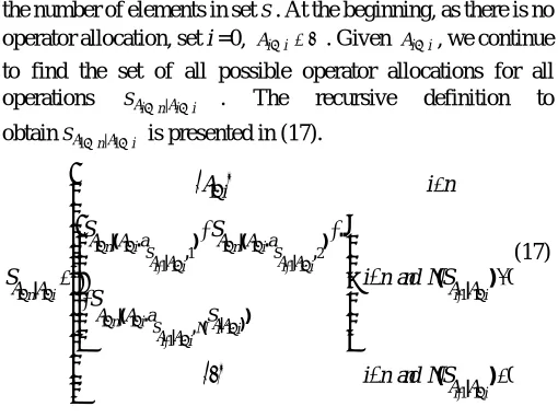
the number of elements in set . At the beginning, as there is no operator allocation, set i =0, . Given , we continue to find the set of all possible operator allocations for all operations . The recursive definition to obtain is presented in (17).
S Φ =
→i i
A Ai→i
i i A n i A
S →| →
i A n A
S1→|1→
{ }
{ }
1 1 1 1 1 2
1 1 1 1
1 1 1 1
1 1 1
1 1 1 1 1 0 0 , , | | | ) , ( | |( . ) |( . ) | | |( . ) | .. ( ) ( )
n iS n iS
A Ai i A Ai i
n i i i
n iSA A N iAAi
i i
i i
i
A A a A A a
A A A A
A A a S
A A
A i n
S S
S i n and NS
S
i n and NS
→ → → → + → + → → → + → → → → + → + → → ⎧ = ⎪ ⎪⎧ + +⎫ ⎪⎪ ⎪ ⎪⎪⎪ ⎪
=⎨⎨ ⎬ < >
+
⎪⎪ ⎪
⎪⎪ ⎪
⎩ ⎭
⎪
⎪ Φ < =
⎪⎩
(17)
B. RecursiveCombinatorialAlgorithm
A general algorithm for obtaining the set of all combinations of any m elements from a set
S
is proposed as follows. It is used in the above operator allocation algorithm to generate the set of all possible combinations of needed multiple-skilled operators for a specific operation.Given . represents the subset of
including the elements from to continuously, that is: , is the union operation of the element with . is the set of all combinations of any m elements from the set S. If given , can be obtained by (18).
} ,..., ,
{as,1as,2 as,N(s)
S= Si→N(S)
S as,j as,N(S)
} ,..., ,
{as,i as,i+1 as,N(s) as,i.as,j
i s
a, as,j CSSm
) (S N i
S→ CSSmi→N(S)
{ } ( )
{
1}
( )1 1 1 2 1 1
1 1 1 1
1 1 1 1 1 2
2 2
0 i n
s i s i s N s i n
s iCSm s iCSm s i m m CS N CS Si N s Si N s Si N s Si N s m
Si N s s i CSm s i CSm s i Si N s Si N s
N S m or m
a a a N S m
a a a a a a
CS a a a a a
φ → + → − − − ⎛⎜ − ⎞⎟ +→ +→ +→ ⎜⎝ +→ ⎟⎠ + − + − + → + → + → < = = = , , , ( ) , , , , , , ( ) ( ) ( ) ( ) , , , ( ) , , ( ) ( ) ... , , ..., , , , ..., ( )
1 1 1
2 2
1 1 1
m m
CSS N CSS i N s i N s
i n
s N s mCSm SN s m N s
a
N S m
a a ⎛ ⎞ − ⎜ − ⎟ ⎜ ⎟ + → ⎝ + → ⎠ → − − − +→ ⎧ ⎪ ⎪ ⎪ ⎪ ⎪ ⎪ ⎪⎧ ⎫ ⎪ ⎪⎪ ⎪⎪ ⎪ ⎪⎪ ⎪ ⎨⎪ ⎪ ⎪⎪
⎪⎪⎪⎪⎨ ⎬ >
⎪⎪ ⎪ ⎪⎪ ⎪⎪ ⎪⎪ ⎪⎪ ⎪⎪ ⎪ ⎪⎪⎩ ⎪ ⎩ , ( ) ( ) , ( ) , ( ) ( ) , ..., ..., ..., opr s N ⎪ ⎪⎪ ⎪ ⎪ ⎪ ⎪ ⎭ (18) C. Optimization
Three optimal indices, namely, efficiency of bottleneck operation (Eff of bottleneck), standard deviation of operation efficiency (Std of opreff), and total operation efficiency waste (total opreff waste), are proposed to evaluate the goodness of a specific operator allocation so as to find the optimal solution.
V. EXPERIMENT AND RESULTS
A. Case of Adjustment for Condition of NSnopr[i] < NSsopr[i]
The following experiment will demonstrate with case 1 the
approach of how to adjust the condition of < . The result of running the adjusted operator allocation optimization algorithm is also reported.
] [i N
nopr
S NSsopr[i]
In this case, before adjustment, the set of all operators is {Opr1, Opr2, Opr3, Opr4, Opr5, Opr6, Opr7, Opr8}, the set of all operations is {Opt1, Opt2, Opt3}, total number of operators is 8 and total number of operations is 3. Skill matrix of each operator ( , , ), and predicted efficiency of operator j on operation i ( ) are shown on left side of table 1 respectively. Based on that SAM= {1.20, 1.60, 1.80} and total operator number is 8, the number set of operators needed for each operation is calculated as {3, 1, 4}. The number of total available operators for each operation is {3,4,4} and the number of single skilled operators for each operation is {1,2,2}.
opr S opt S opt s N ] [i
Sopr Ssopr[i] Smopr[i]
] , [i j Eopr
] [i NSnopr
] [i Nsopr
[image:4.612.46.301.52.243.2] [image:4.612.314.572.302.728.2]] [i NSsopr
Table 1: Condition adjustment for operator allocation in case 1 Before adjustment After adjustment
i j
Opt1 Opt2 Opt3 Opt1 Opt2 Opt3
opr
S
Opr1, Opr2, Opr3, Opr4, Opr5, Opr6, Opr7, Opr8
Opr1, Opr2, Opr3, Opr4, Opr6, Opr7, Opr8
opr s
N 8 7
nopr s N 8 7 ] [i Sopr Opr4, Opr1, Opr7 Opr5, Opr8, Opr1, Opr2, Opr8, Opr7, Opr6, Opr3 Opr4, Opr1, Opr7 Opr8, Opr1, Opr2, Opr8, Opr7, Opr6, Opr3 Opr4 Opr5,
Opr2, Opr6, Opr3
Opr4 Opr2 Opr6, Opr3 ] [i Ssopr Opr1, Opr7 Opr1, Opr8 Opr7, Opr8 Opr1, Opr7 Opr1, Opr8 Opr7, Opr8 ] [i Smopr ] , [i j Eopr 0.40, 0.70, 0.75 1.10, 1.20, 1.30, 1.40 0.20, 0.25, 0.40, 0.50 0.40, 0.70, 0.75 1.20, 1.30, 1.40 0.20, 0.25, 0.40, 0.50 ] , [i j Esopr
0.40 1.10, 1.40
0.40, 0.50
0.40 1.40 0.40, 0.50
] [i SAM
1.20 0.60 1.80 1.20 0.60 1.80
] [i NSnopr
3 1 4 2 1 4
] [i Nsopr
3 4 4 3 3 4
] [i N
sopr
S 1 2 2 1 1 2
] [i
NSnopr 2 2 2 2 2 2
for the second operation 2 is larger than that of operators really needed, 1. No combination is possible to be obtained under this condition. So it has to be adjusted. Using the approach in A part of Section 3, the optimal number of single skilled operators on Opt 2 is achieved as 1. Thus one of the two available single skilled operators, Opr5 and Opr2, has to be removed. As Opr 2’s efficiency is higher than Opr5’s, Opr 5 is hence removed from the set. After recalculation, changes to {2, 1, 4}. to {3, 3, 4} and to {1, 1, 2}. Continue the above steps on all left operations, till all conditions are confirmed to be satisfied. The final result is shown on the right side of Table 1.
] [i NSnopr
] [i
Nsopr NSsopr[i]
After that, run the adjusted operator allocation optimization algorithm to achieve two feasible allocations. The optimal operator allocation is chosen in terms of three indices. Details are shown in Tables 2 and 3.
Table2: Case 1: three indices of the optimal operator allocation Eff of bottleneck Std of opreff total opreff waste
1.15 0.1323 0.45
Table 3: Case 1: the optimal operator allocation
Opt1 Opt2 Opt3
]
[
i
S
noprOpr4, Opr7 Opr2 Opr8,Opr7, Opr6,Opr3
B. Case of Adjustment for Condition of Nsopr[i] < NSnopr[i]
The following experiment will demonstrate with case 2 the approach of how to adjust the condition of <
and report the corresponding result of the optimal operator allocation.
] [i
Nsopr NSnopr[i]
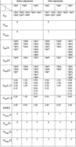
In this case, before adjustment, , , and are the same as Case 1 as shown in table4. Skill matrix and predicted operator efficiency are different. SAM= {2.40, 0.50, 1.00}, and is calculated as {5, 1, 2}. The number of total available operators for each operation is {4,3,6} and the number of single skilled operators for each operation is {1,1,1}. Analysis shows that the number of needed operators for the first operation, 5, is larger than that of all operators available, 4. Using the approach in B part of Section 3, the optimal number of needed operators on Opt 1 is 4. After recalculation, changes to {4, 1, 2}. and keep unchanged. The system continues to check all left operations, till all conditions are satisfied.
opr
S Sopt Nsopr Nsopt
] [i NSnopr
] [i Nsopr
] [i NSsopr
] [i
NSnopr Nsopr[i]
] [i NSsopr
[image:5.612.314.572.64.565.2]An optimal operator allocation is selected from three available allocations after running the adjusted operator allocation optimization algorithm. Three indices and details of the optimal allocation are shown as follows:
Table 4: Condition adjustment for operator allocation in case 2 Before adjustment After adjustment
i j
Opt1 Opt2 Opt3 Opt1 Opt2 Opt3
opr
S
Opr1, Opr2, Opr3, Opr4, Opr5, Opr6, Opr7, Opr8
Opr1, Opr2, Opr3, Opr4, Opr5, Opr6, Opr7, Opr8
opr s
N
8 8
nopr s
N
8 7
] [i Sopr
Opr4, Opr6, Opr5, Opr7
Opr8, Opr1, Opr2,
Opr7, Opr3, Opr2, Opr6, Opr5, Opr8
Opr4, Opr6, Opr5, Opr7
Opr8, Opr1, Opr2,
Opr7, Opr3, Opr2, Opr6, Opr5, Opr8
] [i Ssopr
Opr4 Opr1 Opr3 Opr4 Opr1 Opr3
] [i Smopr
Opr5, Opr6, Opr7
Opr2, Opr8
Opr2, Opr5, Opr6, Opr7, Opr8
Opr5, Opr6, Opr7
Opr2, Opr8
Opr2, Opr5, Opr6, Opr7, Opr8
] , [i j Eopr
0.20, 0.28, 0.30, 0.32
1.25, 1.30, 1.40
0.58, 0.60, 0.65, 0.65, 0.70, 0.72
0.20, 0.28, 0.30, 0.32
1.25, 1.30, 1.40
0.58, 0.60, 0.65, 0.65, 0.70, 0.72
] , [i j Esopr
0.20 1.30 0.60 0.20 1.30 0.60
] [i SAM
2.40 0.50 1.00 2.40 0.50 1.00
] [i NSnopr
5 1 2 4 1 2
] [i N
opr s
4 3 6 4 3 6
] [i NSsopr
1 1 1 1 1 1
] [i NSnopr
3 2 5 3 2 5
Table 5: Case 2: three indices of the optimal operator allocation Eff of bottleneck Std of opreff total opreff waste
1.10 0.1007 0.28
Table 6: Case 2: the optimal operator allocation (Opr 2 is removed in this allocation)
Opt1 Opt2 Opt3
[ ] opr
S i Opr4, Opr6, Opr5, ,Opr7
VI. CONCLUSION
Previous work [6] studied the operator allocation under the satisfied condition and this paper discusses the allocation under two unsatisfied conditions. The difference among them is that all operators selected will be allocated to produce for the new order if condition (3) is satisfied, while under conditions (4) and (5), some of them may have to be removed from the total operators list to meet the condition. The common point relies on the operator allocation principle: to achieve the most balanced assembly line whatever the condition is. Among the most balanced lines generated, that with the highest bottleneck efficiency and lowest operator efficiency waste will be taken as the best solution.
ACKNOWLEDGMENT
Thank Research Grant Council of the Hong Kong Special Administrative Region for supporting my project. Special thanks should be given to my supervisors, Dr. Wong, Prof. Fan and Dr. Chan as well. Thanks for their patient instructions and warm help.
REFERENCES
[1] W.K. Wong, S.Y.S. Leung, and P.Y. Mok, “Development of a genetic optimization approach for balancing an apparel assembly line,” International Journal of Advanced Manufacturing Technology, 2005, DOI: 10.1007/s00170-004-2350-x, 1-8.
[2] S. M. Eom, S. M.Lee, E. B. Kim, & C. Somarajan, “A Survey of Decision Support System Applications (1988-1994) ,” The Journal of the O p e r a t i o n a l R e s e a r c h S o c i e t y , 4 9 ( 2 ) , 1 9 9 8 , p p . 1 0 9 - 1 2 0 [3] Racine, R., Chen, C., & Swift, F. “The impact of operator efficiency on
apparel production planning”. International Journal of Clothing Science and Technology, 4(2/3), 1992, pp.18-25.
[4] B.L. Song, W.K. Wong, J. Fan, and S.F. Chan, “Real-time intelligent optimization decision support system for line-balancing control,” The
proceedings of the 9th World Multi-conference on Systemics, Cybernetics and Informatics, Orlando, Florida, USA, 2005, July 10 – 13.
[5] B.L. Song, W.K. Wong, J. Fan, and S.F. Chan, “Prediction of operator efficiency using time series and artificial neural network techniques,” Computers & Industrial Engineering, 2006, submitted for publication. [6] B.L. Song, W.K. Wong, J. Fan, and S.F. Chan, “A recursive operator allocation approach for assembly line-balancing optimization problem with the consideration of operator efficiency,” Computers & Industrial Engineering, 2006, accepted for publication.