Neural mechanisms involved in error processing: A comparison of errors made with and without awareness

Deriving the optimal number of events for an event-related

fMRI study based on the spatial extent of activation

Kevin Murphy

and Hugh Garavan

*

a

Department of Psychology and Institute of Neuroscience, Trinity College, Dublin 2, Ireland b

Department of Psychiatry and Behavioral Medicine, Medical College of Wisconsin, Milwaukee, WI 53226, USA

Received 20 July 2004; revised 25 April 2005; accepted 5 May 2005

Event-related fMRI is a powerful tool for localising psychological functions to specific brain areas. However, the number of events required to produce stable activation maps is a poorly investigated and understood problem. Huettel and McCarthy [Huettel, S.A., McCarthy, G., 2001. The effects of single-trial averaging upon the spatial extent of fMRI activation. NeuroReport 12, 2411 – 2416] have shown that the spatial extent of activation increases monotonically with the number of events in an analysis. In the present paper, this result is replicated and shown to be a consequence of the cross-correlation technique used to determine active voxels and does not hold, for example, for a GLM analysis. Another analysis technique, that does not depend on good-ness-of-fit to the data, is also proposed. This technique calculates an impulse response function (IRF) for each voxel, finds the best fitting haemodynamic shape to the IRF and returns an area-under-the-curve (%AUC) activation measure. Using spatial extent as a measure, asymptotic behaviour is evident after as few as 25 events for the %AUC analysis technique in a finger-tapping task with non-over-lapping haemodynamic responses and for both the GLM and %AUC techniques in a similar task that allows responses to overlap. The experimental validity of the %AUC technique to identify active brain regions while minimising false positive levels is demonstrated in a group study with 25 participants.

D2005 Elsevier Inc. All rights reserved.

Keywords:Event-related fMRI; Spatial extent

Introduction

Functional magnetic resonance imaging (fMRI) has become a widely employed and useful technique in the field of brain imaging. Its superior spatial resolution allows a researcher to localise functions to specific areas of the brain. Event-related experimental designs, first proposed by Blamire and colleagues

(Blamire et al., 1992), are fast becoming the norm in fMRI. The advantages of event-related over block designs include the ability to randomise behavioural trials thus leading to more complex cognitive tasks (e.g., GO/NOGO, oddball or priming tasks), the ability to remove the influence of incorrect trials from the signal (which has been shown to have detrimental effects on the resulting activation maps; Murphy and Garavan, 2004a) and the ability to examine the temporal dynamics of a response.

Most techniques used to analyse event-related fMRI data assume that the haemodynamic shape of the BOLD signal is linearly additive. However, it has been shown that the haemody-namic shape shows a 17 – 25% reduction in amplitude when trial onsets are spaced (on average) 5 s apart compared to those spaced 20 s apart (Miezin et al., 2000). Therefore, it is very important to determine the optimal interstimulus interval (ISI). Dale demon-strated that if the ISI is jittered, the statistical efficiency improves monotonically with decreasing mean ISI and that the efficiency can be up to 10 times greater than that of a fixed ISI design (Dale, 1999). However, there are two fundamentally different goals when analysing event-related fMRI tasks: estimation of the impulse response function (IRF) and detection of signal change. Birn and colleagues showed that the estimation of the IRF is optimised when stimuli are frequently alternated between task and control states, whereas detection of activated areas is optimised by block designs (Birn et al., 2002). Consequently, an important consideration in designing and analysing event-related studies is that the analysis technique be able to accommodate overlapping haemodynamic responses.

As fMRI is an expensive method, efforts must be made to optimise the design of studies to reduce costs without compromis-ing results. Given these considerations, how many events to include in an event-related experimental design is a pertinent issue but one that has been poorly addressed in the literature. One possible reason for this could be that there is no standard metric by which to measure the required number of events. If one examined how spatial extent of activation varies as the number of events increases, one would expect that as the optimal number of events is reached, the spatial extent would cease to grow. However, it has been shown, in a block design experiment, that when progressively

1053-8119/$ - see front matterD2005 Elsevier Inc. All rights reserved. doi:10.1016/j.neuroimage.2005.05.007

* Corresponding author. Department of Psychology and Institute of Neuroscience, Trinity College Dublin, Dublin 2, Ireland. Fax: +353 1 671 2006.

E-mail address:[email protected] (H. Garavan).

Available online on ScienceDirect (www.sciencedirect.com).

averaging over scans (one scan = 200 s: 20 s ON, 20 s OFF,. . .) the spatial extent of activation increased monotonically and failed to asymptote even after 22 scans (Saad et al., 2003). Huettel and McCarthy have reported a similar result in an event-related task (Huettel and McCarthy, 2001). It was found that at a number of events typical of fMRI experiments (i.e., 50 trials), only 50% of the eventually active voxels were found to show a significant effect. Indeed, the spatial extent of activation failed to asymptote even after 150 events. This would suggest that the number of events required in an event-related study far exceeds practical capabilities and existing conventions.

In this paper, it is proposed that the Huettel and McCarthy result is a consequence of the correlation method used. It is demonstrated that utilising a different technique, first employed by Garavan and colleagues (Garavan et al., 1999), asymptotic values are reached in the range typical of fMRI experiments. Furthermore, in keeping with the advantages of jittering events such that their haemody-namic responses overlap, we demonstrate an early asymptote with both overlapping and non-overlapping haemodynamics.

Materials and methods

Participant and task design

One female right-handed participant (age: 38) completed two event-related finger-tapping tasks. Each task consisted of a black and white flashing checkerboard (4 Hz frequency) lasting 1 s. In the first experiment, this was presented 30 times over a 10-min period with an interval of 20 s between each trial, thus avoiding overlapping haemodynamics (Non-Overlap task). In the second experiment, this was presented 30 times over 6 min at intervals of between 8 and 16 s (Overlap task). A countdown clock was presented prior to each checkerboard presentation to prepare the participant. While the checkerboard appeared on screen, the participant was required to finger-tap bilaterally. Five successive blocks of the first experiment were run, giving 150 finger-tapping events. On a separate day, five blocks of the second experiment were run, also yielding 150 events.

To verify the sensitivity of the different analyses methods used, 25 participants (14 female, mean age: 25, range: 19 – 36) completed one 6-min block of the Overlap task.

Scanning parameters

Scanning was conducted using contiguous 7-mm sagittal slices covering the entire brain from a 1.5-T GE Signa scanner using a blipped gradient-echo, echo-planar pulse sequence (TE = 40 ms; TR = 2000 ms; FOV = 24 cm; 6464 matrix; 3.75 mm3.75 mm in-plane resolution). High-resolution spoiled GRASS ana-tomic images (TR = 24 ms, TE = 5 ms, flip angle = 45-, FOV = 24 cm, thickness = 1.0 mm with no gap, matrix size = 256256

124) were acquired prior to functional imaging.

Image processing

All data processing was conducted using the AFNI software package (Cox, 1996) (http://afni.nimh.nih.gov/afni). Initially, each voxel’s time series was shifted so that the separate slices acquired at varying times were aligned to the same temporal origin. For each task, the five experimental blocks were concatenated into one data

set by removing the mean and linear trend of each block separately, joining the five time series together and reintroducing the overall mean across the five blocks. Each 3D image corresponding to a particular time point was then volume registered to a ‘‘base’’ image using a Fourier interpolation algorithm to align the voxels. Voxels lying outside the brain were removed.

Analysis techniques

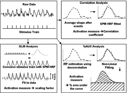
Three types of analyses were performed on the Non-Overlap data (seeFig. 1). First, following Huettel and McCarthy’s technique, a

correlation analysis was performed in which the ten time points (corresponding to 20 s) after each event were averaged across all events for each voxel in the brain. This 20-s long time series was then correlated with a standard haemodynamic shape taken from the Statistical Parametric Mapping package (SPM;http://www.fil.ion. ucl.ac.uk/spm/spm2.html). The correlation coefficient, a goodness-of-fit measure, was used as the activation measure. Second, aGLM analysis was performed in which a regressor was obtained by convolving the event stimulus train with the standard SPM haemodynamic response. A scaling factor for this regressor was found in each voxel using a multiple regression procedure (which also included regressors to remove nuisance terms). This procedure calculates how much it has to ‘‘scale’’ the regressor so that the best fit to the data is found. These scaling factors were then converted into a

Z-score map. Third, a method that can accommodate differences in haemodynamic shape, both within- and between-subject was used. This involved an estimation of the impulse response function (IRF) for each voxel using a deconvolution technique. Using multiple regression techniques (with nuisance regressors included), this procedure calculates the IRF (i.e., the average best-fitting ‘‘shape’’) that follows each event. To achieve this, a regressor that specifies where each event occurs was first defined. This regressor was then time-shifted by 1 TR to create a new regressor that specified events 1 TR later. This was repeated up to 8 TRs (i.e., 16 s). The deconvolution procedure then calculated a scaling value for each regressor using a least-squares multiple regression algorithm and these scalar values defined the IRF for each voxel. The deconvo-lution procedure also calculates intercept and slope parameters, which can be used to calculate a baseline (i.e., the ongoing mean activity level after excluding the variance due to the events) for the IRF. The best fitting haemodynamic shape (a gamma-variate function,y=ktre t/b) was determined for each voxel’s IRF using a non-linear regression algorithm (Ward et al., 1998). The estimated haemodynamic shape for each voxel was converted into a percentage area-under-the-curve score (%AUC) by expressing the area under the haemodynamic curve as a percentage of the area under the baseline. The gamma variate function has been shown to effectively model the haemodynamic response (Cohen, 1997); however, the technique is flexible and another model could be used to find the best-fitting shape, from which a %AUC measure could be calculated. This method was termed the%AUC analysis.

Permutation analyses

Further analyses were carried out to determine the behaviour of activation maps as a function of the number of events. For the Non-Overlap data, twenty random samplings (with replacement) of 5, 10,. . ., 150 events were chosen. The correlation analysis was repeated by averaging over just those events chosen for each sample size. Similarly, the GLM analysis was repeated with a regressor created by convolving the standard haemodynamic shape with the stimulus train consisting only of the events in the sample. All other events were excluded from the analysis by including another regressor in the multiple regression procedure consisting of the convolution of the standard haemodynamic shape with the stimulus train of those events not in the sample. The %AUC analysis used a regressor containing only the events in the sample. Again all other events were excluded from the analysis with a second regressor. This procedure produced 600 activation maps for each analysis type (i.e., 20 maps for each number of events 5, 10,. . ., 150). These activation maps were then thresholded and the number of active voxels in the ROIs derived above was counted. The correlation analysis maps were thresholded atP< 0.001 (t> 3.88341) as inHuettel and McCarthy (2001). The GLM analysis activation maps were also thresholded atP< 0.001 (z= 3.1). The %AUC activation maps were converted into Z scores by calculating the mean and standard deviation of %AUC across all voxels in the brain, then using the formula (%AUC mean)/ (standard deviation) to change each voxel’s %AUC into aZscore. These maps were then thresholded with the sameZvalue as used for the GLM analysis.

Two types of analyses were performed on the Overlap data, the GLM and the %AUC analyses (the correlation analysis was not carried out, as it was impossible to average haemodynamic shapes due to their overlapping characteristics). Activation maps were found that included all 150 events and ROIs (124 voxels) were calculated using the same procedure as above (i.e., voxels in the ROI must be present in the top 10% of both analysis types). Twenty random samples were chosen of 5, 10,. . ., 150 events. Due to the overlapping nature of the haemodynamics, two regressors were made for each analysis type. First, a regressor including all the events in the sample and second, a regressor including all other events so that the contribution of these events to the time series would be removed. The same procedure was followed to determine the behaviour of the activation maps as a function of number of events.

Group analysis

To determine if the %AUC analysis yields similar results to the GLM analysis, the data from the 25 participants were analysed using both approaches. Each data set was then resampled to a higher 1-Al resolution (thus 1 voxel = 1 Al) and converted to the standard stereotaxic coordinate system of Talairach and Tournoux (Talairach and Tournoux, 1988). The images were then spatially smoothed using a Gaussian kernel with 3-mm r.m.s. isotropic deviation. A voxelwise t test was performed on the 25 maps for each analysis type and a threshold of P < 0.00005 with a 100-Al cluster criterion was imposed.

Results and discussion

Non-overlap analysis

The ROIs derived from the three analysis types of the Non-Overlap data comprised an activation map with 115 voxels, mainly situated in left and right primary motor cortex and in the visual cortex. It is important to note that when the activation maps were thresholded atP< 0.001, none of the analyses found all 115 voxels to be statistically significant. This is due to the method used to select the voxels for the ROI (i.e., each included voxel was required only to be in the top 10% of each activation map), which did not depend on significance levels. This procedure resulted in a liberal selection of voxels and guaranteed that all those voxels passing the threshold criterion would be contained within the ROIs.

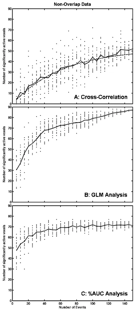
Fig. 2A shows the number of voxels that are found to be significantly active in the ROIs as a function of the number of events using the cross-correlation analysis. The mean of the 20 samples is a monotonically increasing line that appears to be slightly concave. This graph corresponds closely to that found by Huettel and McCarthy, with their derived equation,V=Vmax(1

e( 0.016 N)), fitting well over the mean data points, thus replicating their result.

Fig. 2B shows the same graph for the GLM analysis. This graph monotonically increases as a function of the number of events. However, after 40 events, the slope of the mean line decreases (slope of line before 40 events = 1.0526, slope of line after 40 events = 0.1777). Thus, between 40 and 150 events, the number of significant voxels increased by only 19 (a 27% increase over the 68 voxels that were significant at 40 events).

The graph for the %AUC analysis is quite different (seeFig. 2C). The starting point is greater and the mean number of voxels does not increase quite as quickly as it does for the previous two analyses. Again, there is a dramatic change in slope from 0.5087 before 40 events to almost a flat line slope of 0.0393 thereafter. This demonstrates that, after 40 events, the number of significant voxels increases very little as a function of the number of events using the %AUC method. Indeed, after 40 events, only five fewer voxels are deemed to be significantly active than after 150 events. The mean number of significant voxels after only 5 events is 48 compared with 71 at 150 events.

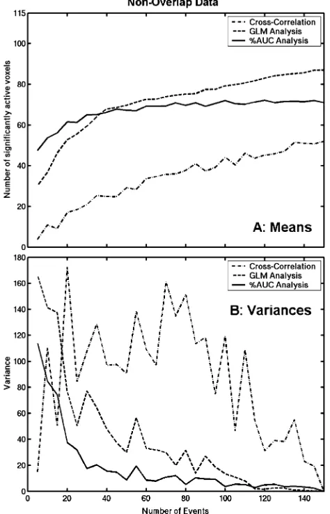
Fig. 3A replots the means of the three analyses together to show how many of the 124 ROI voxels are deemed to be significantly active by each. The %AUC measure performs the best up to 40 events while the GLM analysis performs better thereafter. However, the %AUC analysis has a lower variance across the 20 samples, especially at lower numbers of events (seeFig. 3B).

The reason the %AUC technique, compared to the cross-correlation technique and, to a lesser extent, the GLM analysis, is more powerful at low numbers of events is that it is almost ‘‘blind’’ to noise in the data since it does not depend on a goodness-of-fit measure. To demonstrate the rationale behind this, take one haemodynamic response that is exactly the same as the SPM HRF, but with random Gaussian noise added at each time-point. The cross-correlation technique compares this event with the SPM HRF and will find a poor correlation value because of the included noise. As more and more of these events are averaged together, the random noise will start to cancel out and the average will begin to look like the standard HRF. Thus, the correlation value will increase and the voxel will pass a statistical threshold and be

deemed active. The GLM analysis performs better because it fits its regressor to the time series but then derives an activation measure from the scaling factor that does not depend on the goodness-of-fit.

Fig. 2. The number of significantly active voxels as a function of the number of events is plotted for (A): the cross-correlation analysis, (B): the GLM analysis and (C): the %AUC analysis on the Non-Overlap data. The solid line displays the mean number of voxels over the 20 samples at each event size. The dotted line in panel A shows the equation derived by

Huettel and McCarthy (2001):V=Vmax(1 e( 0.016N)_{), whereVmax=}

However, if the voxel’s IRF is quite different from the standard HRF or if the noise results in a mismatch between the regressor and the signal embedded in the data, then the GLM analysis will have difficulty fitting the regressor to the data, thus compromising the scaling factor. Of course, it should be acknowledged that this situation could be improved by such techniques as adding the first derivative of the regressor in order to accommodate phase-shifting (Calhoun et al., 2004). The %AUC analysis, on the other hand, does not assume a shape for the haemodynamic response. Rather, it fits a gamma variate shape to the central tendency of the data. In a situation in which the central tendency remains unchanged but the amount of noise surrounding it varies, the %AUC measure will be unchanged. As this procedure does not depend on a goodness-of-fit measure of the fitted curve to the data, it should produce relatively stable activation measures with not very many events (assuming that the number of events provide an adequate estimate of the central tendency). This is borne out by the variability in the number of voxels deemed to be significant across the 20 samples. The variation in the cross-correlation data (see Fig. 3B) actually increases as the number of events increases to roughly 75 and then starts to decrease. The spread across the 20 samples is a lot less for the GLM analysis and decreases even further with the %AUC

analysis. Thus, the %AUC technique is more robust and replicable at smaller numbers of events than the other two analysis methods. This explanation might also have implications for the results found bySaad et al. (2003)mentioned earlier. It was found that the spatial extent of activation in a block design increased monotoni-cally as the number of scans included increased. The activation measure in this study was based on the correlation of the time series with a reference block function. If a measure that did not depend on the goodness-of-fit was used instead (e.g., ON – OFF percentage activation change), the spatial extent might asymptote more quickly, thus requiring fewer scans.

Overlap analysis

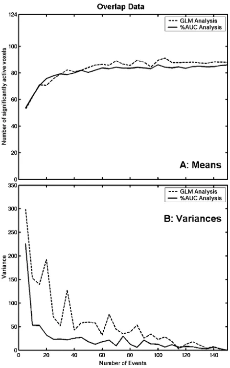
It can be seen fromFig. 4A that the GLM analysis performs better on the Overlap data than on the Non-Overlap data (compare withFig. 2B). There is a sharper rise in the mean number of voxels deemed significantly active at smaller numbers of events after which a shallower asymptote is reached. With 25 events in the analysis, only 13 fewer voxels are deemed active than at 150 events. The overlapping haemodynamic shapes seem to be helping the multiple-regression procedure when it is trying to fit the

Fig. 4. The number of significantly active voxels as a function of the number of events is plotted for (A): the GLM analysis and (B): the %AUC analysis on the Overlap data. The solid line displays the mean number of voxels over the 20 samples at each event size.

convolved regressor to the data. The %AUC analysis also displays an improved performance (seeFig. 4C), possibly because of the greater efficiency afforded by the overlapping design. The asymptote occurs around 25 events where there are 9 fewer voxels deemed active than at 150 events. The mean number of voxels is almost identical between the two analyses methods (seeFig. 5A). However, the variability across the 20 samples using the %AUC method is less than in the GLM analysis (see Fig. 5B). This demonstrates the robustness of the %AUC technique when employed on data with overlapping haemodynamic shapes and suggests that as few as 25 events are sufficient to provide stable activation maps.

The generalisability of the results might be queried since fMRI experiments routinely use more rapid event presentation rates of, say, 2 to 3 s. The %AUC technique depends on an accurate estimation of the impulse response function and it has been shown that estimation accuracy of the haemodynamic IRF actually increases with shorter interstimulus intervals (ISIs) and reaches a maximum at an average ISI of roughly 2 s (Birn et al., 2002). This would suggest that the performance of the %AUC might improve with more rapid presentation rates and that the results are

generalisable to other event-related fMRI experimental designs. However, the Birn paper did not account for additional factors such as the BOLD refractory period that might result in unexpected effects when estimating haemodynamic shapes at shorter presenta-tion rates. Therefore, further empirical analyses are needed to determine if the results of this paper still hold for experiments with more rapid event presentations.

Group comparison

The %AUC technique, which appears to asymptote after as few as 25 events, derives a best-fitting haemodynamic curve for every voxel in the brain and converts it into an activation measure (%AUC). As the curve fitting can be either positive or negative going, returning a positive or negative %AUC value, non-responsive voxels should return a mean of 0 when voxelwise group statistics are performed. Nonetheless, the flexibility of this method may give rise to concerns about high levels of false positives. Therefore, it is important to demonstrate that, in a group study, the technique will determine relevant areas to be active while minimising Type I errors. Twenty-five subjects (the number of subjects established to give stable activation maps;Murphy and Garavan, 2004b) performed one block of the Overlap task (30 events) and were analysed using both the GLM and %AUC analysis techniques. At a threshold ofP < 0.00005 with a cluster criterion of 100Al, the GLM analysis identified an area in the Left Precentral Gyrus [432 Al in size, centred on ( 34, 19,49)] but none in the Right Precentral Gyrus. The %AUC analysis discovered a similar area in the Left Precentral Gyrus [1891 Al in size, centred on ( 30, 24,51)], two in the Right Precentral Gyrus [496 Al in size, centred on (36, 20,40), 419 Al in size, centred on (37, 12,51)] and one in the Right Postcentral Gyrus [484Al in size, centred on (31, 32,52)]. If the cluster criterion is relaxed for the GLM analysis, an area in the Right Precentral Gyrus is found to be active [92Al in size, centred on (37, 20,47)]. The pattern of activation identified by these techniques, being restricted to motor areas, demonstrates the ability of the %AUC measure to identify areas of activation while minimising false positives.

Conclusions

The monotonic increase of the spatial extent of activation as a function of number of events, demonstrated by Huettel and McCarthy (2001), would appear to be a consequence of the cross-correlation method used to determine active voxels. A technique that does not depend on the goodness-of-fit to the data has been proposed that displays the desired effect of reaching an asymptote after what is, experimentally, a more attainable number of events. This %AUC technique, and, perhaps to a lesser extent, the GLM technique, are robust, replicable and can locate func-tionally relevant areas in a group study. The number of events required to yield stable activation maps was determined to be approximately 25, which is well within the practical limits of event-related fMRI studies.

Acknowledgments

Supported in part by USPHS grants DA14100, GCRC M01 RR00058 and by the Irish Research Council for Humanities and

Social Sciences. The assistance of Veronica Dixon is greatly appreciated.

References

Birn, R.M., Cox, R.W., Bandettini, P.A., 2002. Detection versus estimation in event-related fMRI: choosing the optimal stimulus timing. Neuro-Image 15, 252 – 264.

Blamire, A.M., Ogawa, S., Ugurbil, K., Rothman, D., McCarthy, G., Ellermann, J.M., Hyder, F., Rattner, Z., Shulman, R.G., 1992. Dynamic mapping of the human visual cortex by high-speed magnetic resonance imaging. Proc. Natl. Acad. Sci. U. S. A. 89, 11069 – 11073.

Calhoun, V.D., Stevens, M.C., Pearlson, G.D., Kiehl, K.A., 2004. fMRI analysis with the general linear model: removal of latency-induced amplitude bias by incorporation of hemodynamic derivative terms. NeuroImage 22, 252 – 257.

Cohen, M.S., 1997. Parametric analysis of fMRI data using linear systems methods. NeuroImage 6, 93 – 103.

Cox, R., 1996. AFNI: software for analysis and visualization of functional magnetic resonance neuroimages. Comput. Biomed. Res. 29, 162 – 173. Dale, A.M., 1999. Optimal experimental design for event-related fMRI.

Hum. Brain Mapp. 8, 109 – 114.

Garavan, H., Ross, T.J., Stein, E.A., 1999. Right hemispheric dominance of inhibitory control: an event-related functional MRI study. Proc. Natl. Acad. Sci. U. S. A. 96, 8301 – 8306.

Huettel, S.A., McCarthy, G., 2001. The effects of single-trial averaging upon the spatial extent of fMRI activation. NeuroReport 12, 2411 – 2416.

Miezin, F.M., Maccotta, L., Ollinger, J.M., Petersen, S.E., Buckner, R.L., 2000. Characterizing the hemodynamic response: effects of presentation rate, sampling procedure, and the possibility of ordering brain activity based on relative timing. NeuroImage 11, 735 – 759.

Murphy, K., Garavan, H., 2004a. Artifactual fMRI group and condition differences driven by performance confounds. NeuroImage 21, 219 – 228.

Murphy, K., Garavan, H., 2004b. An empirical investigation into the number of subjects required for an event-related fMRI study. Neuro-Image 22, 879 – 885.

Saad, Z.S., Ropella, K.M., DeYoe, E.A., Bandettini, P.A., 2003. The spatial extent of the BOLD response. NeuroImage 19, 132 – 144.

Talairach, J., Tournoux, P., 1988. Co-planar Stereotaxic Atlas of the Human Brain. Theime Medical, New York.