A model based approach for state estimation for networks

(1)

A model-based approach for

state estimation for networks

Orestis Giamarelos

M.Sc. Thesis

January 2018

M.Sc. Thesis Committee:

prof. dr. ir. E. C. van Berkum dr. ir. L. J. J. Wismans ir. O. A. L. Eikenbroek ir. L. C. W. Suijs

(2)

Title: A model-based approach for traffic state estimation for networks

Master Thesis

Author: Orestis Giamarelos

University of Twente

Master’s programme: Civil Engineering & Management

Specialization: Transport Engineering & Management Student number: s1615904

E-mail: [email protected]

(3)

iii

Summary

The aim of this thesis is to develop a model that is able to estimate the traffic state of a network (focusing on urban networks) in real time, by taking into account and fusing traffic data from various sources (e.g. VLOG and Floating Car Data) as they arrive. Most approaches in traffic state estimation focus on freeways and mainly use one source of traffic data. In addition, methodologies designed for use in urban networks usually incorporate a simple node model instead of full modelling of junctions, although the influence of junctions on the traffic state in urban networks is significant. The model developed in this thesis uses Streamline by DAT.Mobility as the process model, which includes detailed modelling of junctions. Data fusion of flow (VLOG) and speed (FCD) data is achieved using Extended Kalman Filtering (EKF).

The model is validated through a series of tests using artificial data (measurements and

“ground truth”). Initially, only one uncertainty parameter is enabled in each test, followed by

combinations of parameters and finally a last test with all uncertainty parameters enabled. The model could satisfactorily estimate the state variables (densities and speeds) of all links of the network, as the average error values of all tests were at an acceptable level.

Estimation improves over time, as the model “learns” through the fusion of measurements.

An increasing uncertainty level of the system leads to a reduced rate of improvement. Estimation of the speeds proved to be more accurate in most validation tests.

The tests also indicated the uncertainty parameters that mostly determine the model’s

performance. Inaccuracy of the measurements (uncertainty and error on the measurements) is the parameter with the highest impact on the results, followed by the inaccuracy of the fundamental diagram parameters and the inaccuracy of the OD matrix. Combinations of these parameters in most (but not all) cases led to an increased combined impact on the state estimation.

Analysis of the most problematic links in each test showed that an inaccurate OD matrix proved to have a higher impact on the estimation of the densities of links connected to a centroid (destination/origin). In addition, in tests with higher uncertainty it was observed that state estimation of links situated on parts of the network where no measurements were available did not improve over time, underlining the importance of the number of measurement points, as well as their position on the network. Among the fundamental diagram parameters, the free flow speed has the most significant impact on the estimation of the speeds and consequently the densities.

(4)

iv of the free flow speed, possibly leading to a higher average error over time. Finally, the inclusion of a warm-up phase, to allow the parameters to approach their actual values, is recommended when possible.

Regarding implementation of the method, it was observed that changing the order of fusing the measurements had practically no impact to the state estimation. In addition, setting reasonable thresholds for the state variables proved to be particularly important, as it can prevent the estimation from diverging, especially in cases with high uncertainty.

Finally, future research suggestions include researching the problem of handling latency and using a different definition for the junction modelling factors, in order to improve fusion of the flow measurements. Moreover, application on a more congested network is

recommended, in order to determine the model’s ability to estimate the speed at capacity

(5)

(6)

(7)

vii

(8)

(9)

ix

Acknowledgements

First and foremost, I would like to express my gratitude to my supervisors:

- Professor Eric van Berkum and Associate Professor Luc Wismans, whose guidance to concretizing the research topic, giving ideas for deeper analysis and finding workarounds whenever my research had reached a dead end was invaluable.

- Oskar Eikenbroek, who devoted a significant amount of his precious time for several months to help me out and often stayed until late at the University working with me to troubleshoot and find bugs in my code. I am grateful for your constant support! - Leon Suijs, who was always available at the company to answer my questions and

help me out. During our scheduled weekly meetings, his valuable feedback always helped my research go further.

Thank you all for your understanding, as well as your insightful comments and suggestions all these months!

A big thank you to DAT.Mobility/Goudappel Coffeng (and Luc Wismans again) for offering me this graduation internship, allowing me to conduct research on a topic of my interest in a great, modern workplace. My thanks also extend to my colleagues at DAT.Mobility. A very special thanks to Jeroen van Oorspronk for devoting so much of his time answering my Streamline and programming questions and creating for me custom Streamline versions with various features whenever needed.

My thanks also extend to the CTS group at the University of Twente for their friendship and support all these months. It was great working and hanging out with all of you!

(10)

(11)

xi

1. Introduction

In the latest years, mobility and logistics have become more important than ever before, especially for economic growth. Subsequently, the significance of road transport has elevated globally. However, this ever-growing demand can often not be efficiently served, as it is in many cases much higher than supply. This imbalance between demand and supply leads to overuse of the existing road network and to widespread congestion, high emissions and noise levels (Calvert el al., 2014). In addition, congestion has proven to be extremely costly for the national economies. According to INRIX (2013), traffic congestion is expected to cumulatively cost for the years 2013-2030 $469 billion to the French national economy, $480 billion to the British, $691 billion to the German and $2.8 trillion to the U.S. economy.

In the past, the most common solution to this problem was to heighten supply levels, by building new roads or by increasing the capacity of the existing network, e.g. by adding extra lanes to existing roads (Wismans et al., 2014). Adding road capacity is no longer a simple solution, as it comes at a high cost and suitable available space is limited. Therefore, effective traffic management becomes increasingly important to maximize the efficiency of the existing road infrastructure.

To achieve the goal of effective traffic management, it is important that adequate information regarding the prevailing traffic conditions is available. Nowadays, a vast and ever-increasing amount of data sources is available, consisting of roadside sensors (e.g. induction loop detectors), in-car sensors (e.g. floating car data) or co-operative roadside and in-car sensors (e.g. automatic vehicle identification via Bluetooth). These data sources can provide information useful to traffic managers, compared to the past when significant effort had to be made to collect measurements and observations from the network. Collection of data has now become easier than ever, but the data coming from many different heterogeneous sources needs to be properly validated (e.g. identifying and removing erroneous measurements and possible systematic errors in the measuring devices) and fused to successfully assess the prevailing traffic conditions and their spatial and temporal dynamics.

(14)

2 maximum density for the Van Aerde fundamental diagram or similar parameters for other fundamental diagram types) etc.

The current state estimates form the basis for (short-term) prediction of the future traffic state of the network. This prediction leads to informed decisions on traffic control measures to be implemented with a typical goal to prevent or minimize congestion (Yuan et al., 2014). The importance of an accurate traffic state estimation is, thus, highlighted by the fact that an inaccurate estimation will propagate through the decision support model, leading to an incorrect prediction of the (near-)future traffic state and to wrong conclusions regarding the appropriate traffic control measures to be used, as the short-term prediction of the future traffic state is a component of major importance for traffic control and ITS (Van Lint & Van Hinsbergen, 2012).

The accurate estimation of the traffic state is not an easy task. Required data is only partially available, in terms of location and time, through sporadically installed sensors (e.g. induction loop detectors) in the road network or through content service providers (e.g. floating car data). The inaccuracy of sensor data available is an additional issue. Significant research has been conducted on the subject and various methodologies have been suggested to improve traffic state estimation. It must be noted, however, that the majority of related work deals with relatively simple freeway networks. In urban networks, complexity of the problem rises significantly due to various factors. For example, the intersections (regulated by traffic signals or unregulated) and the delay they impose to traffic, as well as the calculation of the fraction of traffic flow turning to each direction, are major factors that further increase the complexity of the problem. Other factors that further complicate the problem in urban networks are the following: the higher number of routing options available from origin to destination for each trip, the variation of road users and travel motives, the higher variation in the speeds of the vehicles, the availability of on-street parking and parking garages within the network, as well as the relatively low density of sensors installed in urban networks.

(15)

3

2. Problem Description

As mentioned in the introduction, the term traffic state estimation refers to the estimation of all traffic flow variables necessary to reproduce the traffic conditions on a link or a network, based on available traffic data. Estimation methods include data-driven methods, which use basic statistics, historical data and interpolation based on the sensor data, as well as model-based methods, which also take traffic flow dynamics into account (Yuan, 2013). While the data-driven methods are less complex and computationally expensive than model-based methods, the latter are more accurate and offer the opportunity for full traffic state estimation (e.g. including the fundamental diagram parameters, which are impossible to physically measure), as well as better cope with non-regular traffic conditions. These significant advantages lead to the decision to follow a model-based approach in this research.

A model-based traffic state estimation method consists of three elements (Yuan et al., 2014):

1. A process model, used to predict the state variables (e.g. density, speed, flow). Most

widely used models are the first-order Lighthill–Whitham-Richards (LWR) (Lighthill & Whitham, 1955 and Richards, 1956) and the Cell Transmission Model (CTM) (Daganzo, 1994 & 1995), which is an operationalization of the LWR model. Also used, especially in freeway traffic state estimation, are higher order Payne-type (Payne, 1971) and METANET (Papageorgiou, 1990 and Wang & Papageorgiou, 2005) models.

2. An observation model (measurement functions), used to compute the expected

measurement values to be received from the sensors, considering the uncertainties of the process (e.g. density-flow and density-speed relationships) and the measurements (e.g. due to inefficiencies of the sensors) (Nantes, 2016).

3. A data assimilation/fusion technique, used to estimate the most probable traffic

state by combining the process model predictions, the measurements received from the sensors and the expected measurement values computed by the observation model. There are various data assimilation techniques, employing either simple or more sophisticated algorithms. An example of a simple algorithm is the Newtonian relaxation (nudging) method (Anthes, 1974), which relaxes system models towards observations, thus omitting the necessity for an observation model to perform data assimilation. A popular more sophisticated data assimilation algorithm is the Kalman filtering (KF) method (Kalman, 1960 and Kalman & Bucy, 1961) in various forms, such as the Unscented Kalman Filter (UKF), Ensemble Kalman Filter (EnKF) and especially the more widely used form, which is the Extended Kalman Filter (EKF) (see e.g. Tampère & Immers, 2007, Van Lint et al., 2008, Wang & Papageorgiou, 2005 and Wang et al. 2008).

(16)

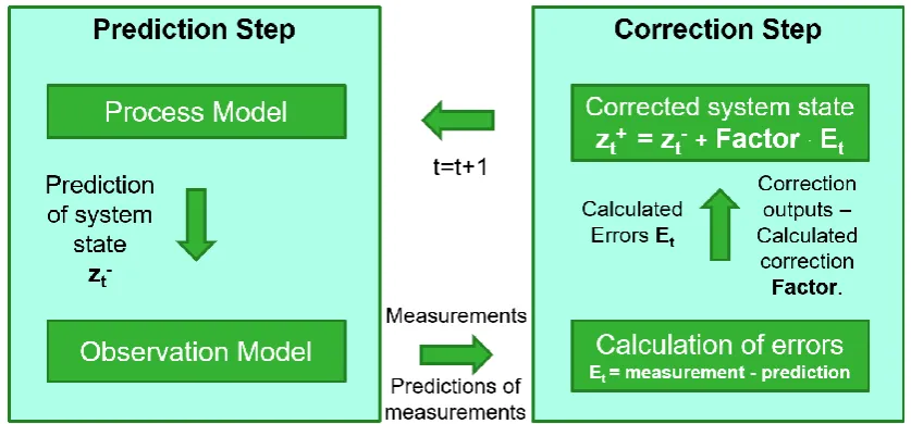
4 each time step. The process model describes the evolution of the system state (e.g. density, speed, fundamental diagram parameters). The observation model relates the system state to the observations. The aim of the data assimilation method is to make an optimal estimation of the system state using all new measurements (observations) that were made available between the previous and the current time step.

For each discrete time step, first a prediction of the system state (𝑧𝑡−) is made, based on the

process model and the last available estimate. Based on this prediction of the state, the observation model predicts the values of the measurements expected to be received from the sensors. In the correction step that follows, the predicted system state is corrected with an optimal weighting factor, proportional to the error (𝐸𝑡) between the predicted

measurement values and the actual measurement values received from the sensors. The optimal weighting factor is determined in terms of minimizing state estimation errors. The corrected state estimate (𝑧𝑡+) is the “belief” of the actual traffic state, as it is the result of the

combination of the process model and the actual measurements. This procedure iteratively provides state estimates at each time step and it is presented in detail in chapter 4.

[image:16.595.87.506.547.742.2]

Most approaches in traffic state estimation use one source of traffic data/observations (Nantes et al., 2016). A possible reason is the complexity of fusing data from different types of sensors into one model: Each data source can possibly have different spatio-temporal resolutions (e.g. Eulerian/Langrangian coordinates). Additionally, it could be difficult to integrate various types of sensor data (e.g. speed, flow, travel time, etc.) into the flow model due to nonlinearities in traffic flow (Wang & Work, 2013). However, as Van Lint & Hoogendoorn (2009) testify, fusing data from multiple sources, when properly performed, leads to a more accurate and robust traffic state estimation.

(17)

5 There are various data sources providing traffic data measurements. The most common are the induction loop detectors, which are roadside sensors that provide flow data. However, there are not enough induction loop detectors installed, especially in urban networks, to rely upon and deliver a full traffic state estimation. The main reason is the high installation and maintenance cost for an adequately dense sensor network. The data they provide is also not entirely reliable, as they are also prone to measurement errors (e.g. Briedis & Samuels, 2010 and Martins, 2008). Errors may occur either due to malfunctioning (e.g. in Herrera et al. (2010) it is mentioned that in California 30% of the 25,000 installed induction loop detectors does not work properly) or due to the nature of the sensor. For example, in a dual induction loop detector setup, a vehicle approaches and changes lane, passing over only one of the two loop detectors of that lane, resulting in an erroneous measurement. Additionally, a single induction loop detector setup requires additional assumptions to be made, e.g. for the average vehicle length. Therefore, uncertainty for the speed measurement values provided by such a setup is higher.

Very common is also the use of Floating Car Data (FCD), which provides instantaneous speed data through GPS-equipped vehicles that transmit their position and speed. The GPS (in)accuracy of 6m (Owens, 1996) or 7.8m with a 95% confidence level (U.S. Department of Defense, 2008) is a drawback of FCD. This accuracy level can be improved using various methods, such as map matching. Other methods offering improved accuracy exist, e.g. Differential GPS and RTK-GPS (Real Time Kinematics) which can offer a typical accuracy of 1.5m and 2cm respectively (van de Pijpekamp, 2015) or an accuracy range of 5m and 1-10cm respectively (Jiménez et al, 2016). However, these methods would require additional equipment to be installed both in-vehicle (e.g. a special antenna) and in the network (reference stations every 100km and 10km respectively). The cost of acquiring floating car data is another drawback, as it is sold by traffic data providers.

Another data source is Bluetooth vehicle identification, which can provide travel times between two specific points in the network. It has the downsides of low penetration rates, high cost of equipment, the uncertain shape and length of the scanning radius, which is based on the surrounding environment (Bhaskar & Chung, 2013) and affects the detection of the vehicles and the measurements (Nantes, 2016).

A less common data source is video image processing (cameras) and automatic number-plate recognition (ANPR). Both sources come at a high cost because of the equipment cost and the fact that they are computationally heavy processes.

(18)

6

3. Research objective and question

The main objective of the proposed research is to develop a model that will be able to

estimate the traffic state of a network (focusing on urban networks) in real time, by taking into account and fusing data arriving from various heterogeneous sources (e.g. VLOG and FCD data) as they arrive. The focus is decided to be on urban networks, as most developed approaches on traffic state estimation focus on freeways (e.g. van Lint & Hoogendoorn, 2009, Wang & Papageorgiou, 2005 and Treiber & Kesting, 2009). Few methodologies, such as the methodology by Nantes et al. (2016), have dealt with urban networks, but still with limitations, such as the lack of a junction model.

An additional objective is to observe if the model is able to cope with situations affecting

supply of infrastructure, e.g. a reduced free flow speed due to fog covering a part of a large network or a reduced capacity on a link due to an incident. Therefore, the additional objective is to observe if the fundamental diagram parameters, the parameters that determine the shape of the fundamental diagram, can also be accurately estimated by the model.

The main research question, deduced from the main objective, is the following:

How can a model be developed to provide online estimation of the traffic state of an urban network, taking into account measurements from sensors?

An additional research question, covering the additional objective, is the following:

How accurately can this developed model estimate the fundamental diagram parameters of each link of the network?

The key terms of the research questions are the following:

The traffic state is defined as the densities and speeds of each link, which lead to the estimation of the flows as well, assuming homogeneity of traffic. As the additional research question also requires the fundamental diagram parameters to be estimated, the traffic state has to include these parameters as well.

The term sensors refers to measurements coming from sensors installed either roadside (e.g. directional flows derived from VLOG data) or onboard the vehicles (e.g. link speeds derived from FCD). As sensors are not perfect, sensor reliability is also a factor that must be considered in the development of the method.

(19)

7 assumed that there is no latency in the measurement values received. This means that a measurement of e.g. the average directional flow for a whole minute is made available immediately, exactly at the end of the 60th_{second of that minute.}

The fact that the methodology must be suitable for urban networksincreases the complexity of the research problem. Urban links are more challenging to model than freeway links, due to, e.g., the more complex traffic dynamics at intersections and the existence of unregulated intersections, which add a significant amount of uncertainty to the traffic state estimation. The junctions play a very determining role in urban networks, so the developed methodology should be able to cope with junctions. Therefore, junction modelling, as part of the model prediction is essential.

Thus, in order to address this problem, the developed model should be accurate, fast enough, dependent only on the observations available until the current time step (no pre-processing of measurements required), able to accommodate all junction types, estimate supply (fundamental diagram) parameters online and handle the uncertainties of model inaccuracies and sensor reliability.

(20)

8

4. Method

4.1. Introduction

To address the solution of this problem, referring to the elements of a model-based approach for traffic state estimation, mentioned in chapter 2, and taking into account the analysis of the research questions in the previous chapter, the following decisions were made:

- Streamline, a dynamic traffic propagation model based on METANET and implemented in the transport simulation software OmniTRANS by DAT.Mobility, was selected as the process model. It is a validated model that has been used in the industry for years and it is more complex and accurate than, for example, implementing a simple first-order LWR model. It additionally includes the powerful junction modeling module (XSTREAM), which provides additional opportunities to incorporate high levels of detail when modeling junctions, in order to simulate the actual situation of an urban network as accurately as possible.

- The measurement functions for the observation model will be set up according to the equations used in the process model and the available data sources.

- Finally, the Extended Kalman Filter (EKF), coded in Matlab, is selected as the data

assimilation technique, as it is suitable for working with non-linear equations. In

addition, it is more computationally efficient than other forms, which makes it a good choice for use in large networks (Yuan, 2013), as well as online applications because of the lower computational time it requires. More specifically, a slight modification of the standard EKF algorithm is selected, the incremental EKF proposed by Nantes et al. (2016), which allows incorporating of the various heterogeneous measurements incrementally, whenever they become available, enabling the use of varying sampling rates per data source. Therefore, this methodology offers additional flexibility in relation to the setup of the sensors.

The developed solution is depicted in a flowchart (Figure 2) and the methodology is described in detail in the subchapters that follow.

4.2. Process model

(21)

(22)

10 Each link 𝑖 is designed to have a distance 𝐿𝑖 and the simulation time is divided in time steps

of time 𝑇, so as to satisfy the Courant-Friedrichs-Lewy condition (Sod, 1985). This condition ensures that the distance covered within a time step, which is equal to the free flow speed

(𝑣𝑓𝑟𝑒𝑒₎_{multiplied by the duration of the time step}_𝑇_{, cannot exceed the length of the link}

(𝜐_𝑖𝑓𝑟𝑒𝑒∙ 𝑇 ≤ 𝐿𝑖).

The equations used in the process model are the METANET (Technical University of Crete & Messmer, 2012) equations for the outflow, density propagation and speed propagation. These are presented below:

The outflow of each link 𝑖at time 𝑘 is given by the equation:

𝑞𝑖(𝑘) = 𝜌𝑖(𝑘) ∙ 𝜐𝑖(𝑘) ∙ 𝜆𝑖 , (1)

where

𝑞𝑖(𝑘) denotes the total outflow of link 𝑖 at time 𝑘,

𝜌𝑖(𝑘) denotes the density per lane of link 𝑖 at time 𝑘,

𝜐𝑖(𝑘) denotes the speed of link 𝑖 at time 𝑘 and

𝜆𝑖 denotes the number of lanes of link 𝑖.

The density of each link 𝑖at time 𝑘 + 1 is given by the equation:

𝜌𝑖(𝑘 + 1) = 𝜌𝑖(𝑘) + 𝑇

𝐿𝑖𝜆𝑖(𝑞𝑖−1(𝑘) − 𝑞𝑖(𝑘)), (2)

whose intuitive, physical meaning is that the density of the link at the next time step is the sum of the density at the current time step and the difference between the inflow to link 𝑖

(outflow of the upstream link 𝑖 − 1) and the outflow from link 𝑖.

The speed of each link 𝑖at time 𝑘 + 1 is given by its speed at time 𝑘, plus a relaxation term

that includes a fundamental diagram calculation 𝑉(𝜌), a convection term that expresses the change in speed caused by the inflow of vehicles and an anticipation term that expresses the speed decrease caused by a density increase downstream. The relevant equation is the following:

𝜐𝑖(𝑘 + 1) = 𝜐𝑖(𝑘) +

𝑇

𝜏(𝑉(𝜌𝑖(𝑘)) − 𝜐𝑖(𝑘)) + 𝑇 𝐿𝑖

𝜐𝑖(𝑘)(𝜐𝑖−1(𝑘) − 𝜐𝑖(𝑘))

−𝜈𝛵 𝜏𝐿𝑖

𝜌𝑖+1(𝑘) − 𝜌𝑖(𝑘)

𝜌𝑖(𝑘) + 𝜅

(3)

where τ, ν and κ are model parameters.

(23)

[image:23.595.119.437.71.268.2]

11

Figure 3. The METANET fundamental diagram.

The equation of the METANET fundamental diagram is the following:

𝑉(𝜌𝑖(𝑘)) = 𝜐𝑓𝑟𝑒𝑒∙ exp⁡[− 1 𝛼𝑚∙ (

𝜌𝑖(𝑘) 𝜌𝑐𝑟𝑖𝑡,𝑖(𝑘))

𝛼_𝑚

], (4)

where 𝜌𝑐𝑟𝑖𝑡 signifies the critical density, which can be expressed as:

𝜌𝑐𝑟𝑖𝑡 = 𝑓𝑐𝑎𝑝

𝜐𝑐𝑎𝑝, (5)

where 𝑓𝑐𝑎𝑝 signifies the capacity per lane and 𝜐𝑐𝑎𝑝 signifies the speed at capacity.

The term 𝛼𝑚 is defined as:

𝛼𝑚 = − 1

𝑙𝑛( 𝑓𝑐𝑎𝑝 𝜐𝑓𝑟𝑒𝑒∙𝜌𝑐𝑟𝑖𝑡)

(6)

and using (5):

𝛼𝑚 = − 1

𝑙𝑛(𝜐𝑐𝑎𝑝 𝜐𝑓𝑟𝑒𝑒)

(7)

Therefore, the fundamental diagram equation (4), using (5) and (7) becomes:

𝑉(𝜌𝑖(𝑘)) = 𝜐𝑓𝑟𝑒𝑒∙ exp⁡[𝑙𝑛 ( 𝜐𝑐𝑎𝑝 𝜐𝑓𝑟𝑒𝑒) ∙ (

𝜌_𝑖(𝑘)∙𝜐𝑐𝑎𝑝 𝑓𝑐𝑎𝑝 )

− 1 𝑙𝑛(𝜐𝑐𝑎𝑝

𝜐𝑓𝑟𝑒𝑒)] (8)

4.3. Full state vector

In order to form the full state vector, the approach and the annotations used in Wang & Papageorgiou (2005) will be followed.

The full state vector⁡𝑥 has the following general form:

𝑥 = (𝑙, 𝑑, 𝑝), (9)

(24)

12 The flow 𝑞𝑖(𝑘) for every link 𝑖 at time 𝑘 can be calculated from (1) by replacing the values of

𝜌𝑖(𝑘) and 𝜐𝑖(𝑘) from equations (2) and (3). Therefore, the independent link variables for

each link 𝑖 are 𝜌𝑖 and 𝜐𝑖.

Consequently, the vector of the link variables for a network consisting of 𝑁 links has 2𝑁

elements in total and the following form:

𝑙 = (𝜌1, 𝜐1, 𝜌2, 𝜐2, … , 𝜌𝛮, 𝜐𝛮) (10)

For the calculation of 𝜌𝑖(𝑘 + 1) from equation (2) and the calculation of 𝜐𝑖(𝑘 + 1) from

equation (3), the variables 𝑞𝑖−1(𝑘), 𝜐𝑖−1(𝑘) and 𝜌𝑖+1(𝑘) are also required to be available for

all links. These values can be calculated for all links, except the links at the edges of the network, which have a centroid either as an origin or a destination of the link. Therefore, for all centroids, through which traffic enters and exits the network, the variables 𝑞𝑖−1(𝑘),

𝜐𝑖−1(𝑘) and 𝜌𝑖+1(𝑘) need to be provided as well, in order to enable the estimation of the

link variables for all links of the network. The vector of the boundary variables for 𝐶

centroids has the following form:

𝑑 = (𝑞₁𝑜𝑟𝑖𝑔𝑖𝑛, 𝜐₁𝑜𝑟𝑖𝑔𝑖𝑛, 𝜌1𝑑𝑒𝑠𝑡𝑖𝑛𝑎𝑡𝑖𝑜𝑛, . . . , 𝑞𝐶 𝑜𝑟𝑖𝑔𝑖𝑛

, 𝜐_𝐶𝑜𝑟𝑖𝑔𝑖𝑛, 𝜌𝐶𝑑𝑒𝑠𝑡𝑖𝑛𝑎𝑡𝑖𝑜𝑛) (11)

In Streamline, the convection and anticipation terms of the speed equation (3) containing the variables 𝜐𝑖−1(𝑘) and 𝜌𝑖+1(𝑘) respectively, are omitted from the equation when the

upstream link is an origin and the downstream link is a destination respectively. Therefore, the variables that give the upstream speed of an origin and the downstream density of the destination, are omitted from (11).

The flow entering the network from the origins is modeled with a simple queue model. It mainly depends on the demand, which is read from the OD matrix/matrices Streamline uses to route traffic in the network for the duration of the simulation. The OD matrices are estimated from a variety of data sources such as home and roadside interviews, historical traffic data and observed link volumes. As matrix estimation is beyond the scope of this thesis, it is assumed that the provided OD matrices for the test network are accurate. Therefore, the origin flows can be considered as input to the system, provided by Streamline every time step, and not a state variable.

Thus, no boundary variable is part of the state vector in the developed model, as the upstream speed of the origins and the downstream density of the destinations are omitted in Streamline, while the flow of the origins is input to the system. Therefore, 𝑑 = Ø.

Finally, the fundamental diagram calculation in (8) requires the values of additional parameters, which determine the shape of the fundamental diagram. The three parameters required for the fundamental diagram calculation are the free flow speed (𝑣𝑓𝑟𝑒𝑒_{), the}

capacity per lane (𝑓𝑐𝑎𝑝_{) and the speed at capacity (}_𝜐𝑐𝑎𝑝_{). In a large network, the values of}

(25)

13 fundamental diagram parameters could be affected by various factors, such as adverse weather conditions, which could affect differently the values of the fundamental diagram parameters of each link. For example, fog could be covering only a part of a large network, causing a significant decrease of the free flow speed to the links of that area, while in other areas of the network there could be no or very little decrease of the free flow speed due to the fog. Therefore, it is considered important to set different fundamental diagram parameters for each link and include them in the state vector. The vector of fundamental diagram parameters for a network consisting of 𝑁 links has 3𝑁 elements in total and the following form:

𝑝 = (𝜐₁𝑓𝑟𝑒𝑒, . . . , 𝜐_𝑁𝑓𝑟𝑒𝑒, 𝑓₁𝑐𝑎𝑝⁡, . . . , 𝑓_𝑁𝑐𝑎𝑝, 𝜐₁𝑐𝑎𝑝, . . . , 𝜐_𝑁𝑐𝑎𝑝) (12)

Based on the analysis above, the full state vector 𝑥 for the model consists of 5𝑁 elements and it is presented in (13):

𝑥 = (𝜌1, 𝜐1, . . . , 𝜌𝛮, 𝜐𝛮, 𝜐1 𝑓𝑟𝑒𝑒

, . . . , 𝜐_𝑁𝑓𝑟𝑒𝑒, 𝑓₁𝑐𝑎𝑝⁡, . . . , 𝑓_𝑁𝑐𝑎𝑝, 𝜐₁𝑐𝑎𝑝, . . . , 𝜐_𝑁𝑐𝑎𝑝) (13)

4.4. Full transition model

By replacing equation (1) into equation (2), we receive the following equation for the density:

𝜌𝑖(𝑘 + 1) = 𝜌𝑖(𝑘) + 𝑇

𝐿𝑖𝜆𝑖(𝜌𝑖−1(𝑘) ∙ 𝜐𝑖−1(𝑘) ∙ 𝜆𝑖−1− 𝜌𝑖(𝑘) ∙ 𝜐𝑖(𝑘) ∙ 𝜆𝑖) + 𝜉

𝑞_(𝑘) ₍₁₄₎

The density equation is modelled exact, as it describes the conservation of vehicles. However, the term 𝜉𝑞(𝑘) is added after incorporating the flow equation (1), to reflect the modelling inaccuracy of the approximate flow equation.

Similarly, the term 𝜉𝜐_(𝑘)_{is added to the empirical speed equation (3) to reflect the}

modelling inaccuracy of this equation. The resulting equation is the following:

𝜐𝑖(𝑘 + 1) = 𝜐𝑖(𝑘) +

𝑇

𝜏(𝑉(𝜌𝑖(𝑘)) − 𝜐𝑖(𝑘)) + 𝑇 𝐿𝑖

𝜐𝑖(𝑘)(𝜐𝑖−1(𝑘) − 𝜐𝑖(𝑘))

−𝜈𝛵 𝜏𝐿𝑖

𝜌𝑖+1(𝑘) − 𝜌𝑖(𝑘)

𝜌𝑖(𝑘) + 𝜅

+ 𝜉𝜐(𝑘)

(15)

Therefore, the transition model for the link variables can be written in a compact form as follows:

(26)

14 Or using vectors:

[𝜌𝑖(𝑘 + 1) 𝜐𝑖(𝑘 + 1)] = [

𝜌𝑖(𝑘) 𝜐𝑖(𝑘)] +

[

𝑇 𝐿𝑖𝜆𝑖

(𝜌_𝑖−1(𝑘) ∙ 𝜐_𝑖−1(𝑘) ∙ 𝜆_𝑖−1− 𝜌𝑖(𝑘) ∙ 𝜐𝑖(𝑘) ∙ 𝜆𝑖)

𝑇

𝜏(𝑉(𝜌𝑖(𝑘)) − 𝜐𝑖(𝑘)) + 𝑇 𝐿𝑖𝜐𝑖

(𝑘)(𝜐𝑖−1(𝑘) − 𝜐𝑖(𝑘)) − 𝜈𝛵 𝜏𝐿𝑖

𝜌𝑖+1(𝑘) − 𝜌𝑖(𝑘) 𝜌𝑖(𝑘) + 𝜅 ]

+ [𝜉 𝑞_(𝑘) 𝜉𝜐_(𝑘)]

(17)

The fundamental diagram parameters are modeled with a random walk strategy, meaning that the current value of a variable is composed of the past value plus an error term defined as zero-mean Gaussian white noise:

𝑝(𝑘 + 1) = 𝑝(𝑘) + 𝜉(𝑘) (18)

Or using vectors:

[

𝜐𝑓𝑟𝑒𝑒(𝑘 + 1) 𝑓𝑐𝑎𝑝(𝑘 + 1) 𝜐𝑐𝑎𝑝(𝑘 + 1)

] = [

𝜐𝑓𝑟𝑒𝑒(𝑘) 𝑓𝑐𝑎𝑝(𝑘) 𝜐𝑐𝑎𝑝(𝑘)

] + [

𝜉𝜐𝑓𝑟𝑒𝑒(𝑘) 𝜉𝑓𝑐𝑎𝑝(𝑘) 𝜉𝜐𝑐𝑎𝑝(𝑘)

] (19)

All 𝜉 terms in equations (14)-(19) denote zero-mean Gaussian white noise processes. They are defined as:

𝜉∗= 𝒩(0, 𝜎∗2), (20)

where 𝜎∗ denotes the standard deviation of link variable/fundamental diagram parameter *. The standard deviation for each variable must be set according to the typical time variations expected to be observed in the respective variables/model parameters to be tracked. A higher noise standard deviation for an estimated model parameter indicates a parameter that is more time variant. Thus, a lower standard deviation value would lead to slower convergence of the parameter estimates, while a higher standard deviation value would lead to more nervous behavior (larger fluctuations) of the parameter estimates.

4.5. Junction modeling

Signalized and unsignalized junctions are integral elements of urban networks. Therefore, for a model that can be applied to urban networks, handling junctions is essential. OmniTRANS incorporates XSTREAM, a powerful junction modeling module, which can be used to model signalized junctions and roundabouts, as well as uncontrolled or sign-controlled junctions. It calculates the average delay for each turning movement based on the junction layout, turning flows and signal settings (for signalized junctions).

XSTREAM adds extra turning links to the network with properties that affect traffic propagation accordingly. The data received as output is practically limited to the outflow, speed and density of these extra turning links.

(27)

15 The workaround to this problem is to sum up the effect of junction modeling using appropriate factors, by exploiting the information obtained from Streamline for the state of the next time step (second). Two points are of interest for the state estimation problem: 1. The possible reaching of an outflow limit on the link upstream the junction, as a result of

the traffic light ahead and possibly congestion spillback from the link downstream the turn.

2. The inflow that enters the link downstream the turn, which is affected by the turn delay imposed by junction modeling, as well as the turning fractions.

Therefore, if it is possible to get the information regarding these two points for every time step, the actual details of the calculations made within the junction modeling module are not necessary.

The process used for receiving these factors that sum up the effects of junction modeling is presented below:

1. A factor that summarizes the effect of the first point (using the term “outflow limit

factor”) is received by examining the Streamline state of the next time step. If the flow is

not equal to the product of density, speed and the number of lanes, as in equation (1), then an outflow limit because of either the traffic light or congestion downstream has been reached. So, the outflow limit factor will be equal to 1, unless an outflow limit has been reached, in which case the factor will be less than 1 and calculated as:

𝛼𝑖(𝑘) =

𝑞𝑖(𝑘)

𝜌𝑖(𝑘)∙𝜐𝑖(𝑘)∙𝜆𝑖, (21)

where 𝛼𝑖 signifies the outflow limit factor.

The flow equation (1) is modified to include the outflow limit factor, to reflect the limited outflow when an outflow limit has been reached, taking the following form:

𝑞𝑖(𝑘) = 𝜌𝑖(𝑘) ∙ 𝜐𝑖(𝑘) ∙ 𝜆𝑖∙ 𝛼𝑖 (22)

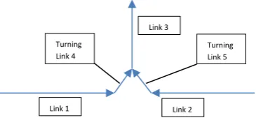
[image:27.595.141.324.579.670.2]

2. The second point affects the inflow of the links downstream the turn. The inflow of this link is the sum of the outflows of the extra turning links that enter this link. The outflows of the extra turning links can be expressed using factors that relate them to the outflow of their upstream link. Consider the junction in the example below:

Figure 4. Example junction.

In this example, the inflow of link 3 will be equal to the sum of the outflows of turning links 4 and 5. However, these can be expressed using a factor that relates them to the outflows of links 1 and 2 respectively. With the Streamline state of the next time step

Turning Link 4

Link 1

Link 3

(28)

16 known, we can calculate these factors and end up with an equation that only contains standard network links (no turning links) and incorporates the effects of junction modeling.

Therefore, for the example junction of Figure 4:

𝑞3𝑖𝑛= 𝑞4𝑜𝑢𝑡+ 𝑞5𝑜𝑢𝑡= 𝛽4∙ 𝑞1𝑜𝑢𝑡+ 𝛽5∙ 𝑞2𝑜𝑢𝑡, where the factors 𝛽 are calculated as 𝛽 = 𝑞_{𝑡𝑢𝑟𝑛𝑖𝑛𝑔⁡𝑙𝑖𝑛𝑘}𝑜𝑢𝑡

𝑞_{𝑛𝑒𝑡𝑤𝑜𝑟𝑘⁡𝑙𝑖𝑛𝑘}𝑜𝑢𝑡 . So, in this example, 𝛽4= 𝑞₄𝑜𝑢𝑡

𝑞₁𝑜𝑢𝑡 and 𝛽5= 𝑞₅𝑜𝑢𝑡

𝑞₂𝑜𝑢𝑡. The values of the factors are

calculated using the Streamline state of the next second (simulation time step), which is known, and their values are replaced in the equation which will be used for this time step.

Thus, the outflows of the turning link 𝑗, which is located downstream network link 𝑖, can be expressed as:

𝑞_𝑗𝑜𝑢𝑡(𝑘) = 𝜌𝑖(𝑘) ∙ 𝜐𝑖(𝑘) ∙ 𝜆𝑖∙ 𝛼𝑖∙ 𝛽𝑗 (23)

These modified flow equations (22, 23) are also used in all equations that include flows, for example in the density equation (2), as well as in the flow measurement functions that will be presented in the next subchapter.

The advantages of using this approach are the following:

• Full XSTREAM settings and features can be enabled and any combination of options for turning delays and traffic light timings may be used.

• The dependencies between the previous and next links of the network are preserved.

• Significantly easier implementation than attempting to implement the full XSTREAM module in the developed model.

The main disadvantage is that the factors need to be recalculated every time step and their values must be updated in all equations and their jacobians. This costs some additional running time, but this process is still faster overall, as with this solution the equations used in the model remain simpler and are therefore faster to calculate.

It has to be noted that the method described calculates the factors using data of the last two consecutive seconds, which leads to capturing the effect of junction modelling on the exact second the EKF is applied. However, for technical reasons it was decided to use average minute data for the calculation of the junction modelling factors. This approach solved a technical problem but led to an inaccuracy in the calculations, which is in most cases negligible, except in cases of sharp increases/decreases of the density.

(29)

17 exceeded the maximum density value, so this behavior is reasonable, as a precautionary measure to allow the density to fall back to acceptable levels (less than the maximum density). However, the initial use of per second data to calculate the factors would in that case possibly be using an outflow of zero, which would lead to the calculation of a factor with a value of zero and eventually zeroing out the whole flow equation and producing wrong estimates of the state variables. To prevent this problem from occurring, it was decided to use average data of the whole minute for the calculation of the junction modelling factors. While the effect of this averaging of data over a minute does not lead to an observable difference in uncongested conditions, it does cause a slight temporary difference, especially to the estimation of the density when congestion is forming and dissolving rapidly, due to e.g. a sharp increase/decrease in demand. When an increase in

density takes place, the “outflow limit factor” is relatively underestimated (depending on

how sharp the increase is), because the average density of 1 minute is a value, which is lower than the density of the last second that should have been used instead. Therefore, an underestimated factor for the same flow will lead to an overestimated density, in order for the flow equation to be valid. The opposite effect is observed, but to a significantly lower extent, in case of an equally sharp dissolving of congestion.

4.6. Measurement functions

With the measurement functions ℎ, the expected value of the measurements from the sensors are expressed, based on the state of the system and the system input. The measurement functions generally consist of the predicted values, adding the uncertainties of the process and the measurement.

The speed measurements are given from Floating Car Data. The speed measurement

function for link 𝑖 is given by the speed plus measurement noise:

ℎ𝑣_𝑖(𝑘) = 𝑣𝑖(𝑘) + 𝛾𝑖𝜐(𝑘), (24)

where 𝛾_𝑖𝜐 denotes speed measurement noise which is modeled as zero-mean Gaussian white noise, similarly to the 𝜉 values in (20).

The flow measurements are available from VLOG data at the stop line of the regulated

intersections. The VLOG data gives the outflow of the turning links, so the relevant flow measurement function is derived from (23):

ℎ_𝑞

𝑗

𝑜𝑢𝑡(𝑘) = 𝜌_𝑖(𝑘) ∙ 𝜐_𝑖(𝑘) ∙ 𝜆_𝑖∙ 𝛼_𝑖∙ 𝛽_𝑗+ 𝜉𝑞(𝑘) + 𝛾_𝑗𝑞(𝑘), (25)

where 𝜉𝑞_(𝑘)_{reflects the modeling inaccuracy of the flow equation, as previously}

mentioned, and 𝛾_𝑗𝑞(𝑘) denotes the flow measurement noise which is modeled as zero-mean Gaussian white noise.

(30)

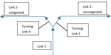
18 junction, where the flow could be limited e.g. only to one direction, due to congestion downstream that direction. In this case, the use of this common factor to each directional flow separately would be wrong, as the actual outflow limit factor to the congested direction should have an even lower value, while the flow limit factors to the other directions could even be 1 (totally unrestricted), depending on the traffic conditions downstream and the demand toward these directions.

To take into account these cases as well, it was decided to use the sum of all directional flows of the entering links to a junction (summing up the measurement values and the respective measurement functions), instead of fusing each individual directional flow measurement separately.

[image:30.595.148.331.430.520.2]

Therefore, for the example junction presented in Figure 5, there are measurements from VLOG data available for the outflows of turning links 4 and 5. The outflow limit factor of link 1 is calculated on the total outflow of link 1, which is divided to the turning links 4 and 5. However, as link 2 is congested and link 3 is not, and depending on the demand to each direction, it is possible that the outflow is limited to only one of these directions or that it is unevenly restricted. The solution to this problem is to sum the measurement values of the outflows of the turning links 4 and 5 and also combine the respective measurement functions, in order to form one combined measurement to fuse using the Extended Kalman Filter.

Figure 5. Example junction.

The individual measurement functions for links 4 and 5 would have been (based on equation 25) the following:

• ℎ_𝑞

4𝑜𝑢𝑡(𝑘) = 𝜌1(𝑘) ∙ 𝜐1(𝑘) ∙ 𝜆1∙ 𝛼1∙ 𝛽4+ 𝜉

𝑞_{(𝑘) + 𝛾} 4

𝑞

(𝑘) for link 4

• ℎ_𝑞

5𝑜𝑢𝑡(𝑘) = 𝜌1(𝑘) ∙ 𝜐1(𝑘) ∙ 𝜆1∙ 𝛼1∙ 𝛽5+ 𝜉

𝑞_{(𝑘) + 𝛾} 5

𝑞

(𝑘) for link 5.

The combined measurement function for the total outflow of the entering link 1 to the junction is the following:

• ℎ_𝑞

1𝑜𝑢𝑡(𝑘) = 𝜌1(𝑘) ∙ 𝜐1(𝑘) ∙ 𝜆1∙ 𝛼1∙ (𝛽4+ 𝛽5) + 𝜉

𝑞_{(𝑘) + 𝛾} 4

𝑞_{(𝑘) + 𝛾} 5 𝑞 (𝑘) Turning Link 4 Link 1 Link 2 -

congested

Turning Link 5

(31)

19 Notice in the combined measurement function the participation of the process noise once (which refers to the modelling inaccuracy of the flow equation) and the measurement noise of all involved sensors (in this example, 𝛾₄𝑞(𝑘) and 𝛾₅𝑞(𝑘)).

A drawback of this approach is that the number of flow measurements to be assimilated in every time step is now reduced. Therefore, the information the Kalman filter obtains from VLOG data is slightly deteriorated, as it comes in the form of a more complex function with more uncertainty parameters included (e.g. all measurement noise elements in one function). Therefore, capturing the errors and error covariances by the Kalman filter is with this approach more difficult, compared to an approach which would use separate flow measurement functions for each measurement.

Finally, it must be noted that the standard deviation values set for 𝛾_𝑗𝑞 and 𝛾_𝑗𝜐 should reflect the reliability level of the corresponding measurements and they depend on the reliability of the sensors. Their values can optionally be different per link, reflecting different accuracy levels of different sensor types that could possibly be installed throughout the network.

4.7. Data fusion using Extended Kalman Filtering

The Extended Kalman Filter has been selected as a computationally efficient data assimilation method. More specifically, the incremental Extended Kalman Filter algorithm has been selected. This slightly modified EKF algorithm, proposed by Nantes et al. (2016), is implemented to handle measurements with different sampling frequencies (e.g. loop detector data aggregated every minute while instantaneous speed data from the floating cars can be available every 15 seconds). The filter adds measurements as they are received without a state transition in-between every measurement. A precondition for this incremental addition of information from multiple measurements is the assumption that all measurements 𝑧 are independent, given the current state and input vectors.

Based on the previously described formulation of the model, the equations are applied to the EKF algorithm (Nantes, 2016).

Definitions:

The state-space model consists of the following equations in compact form:

𝑥(𝑘) = 𝑓(𝑥(𝑘 − 1)) + 𝜉 (26)

𝑧(𝑘) = ℎ(𝑘, 𝑥(𝑘)) + 𝛾 (27) Equation (26) is formed by combining (17) and (19), while equation (27) is formed by combining (24) and (25).

The process noise covariance matrix is defined as:

𝑇 = 𝑑𝑖𝑎𝑔(𝜉) (28)

(32)

20 The Jacobian of the state transition function 𝑓, with respect to the full state vector 𝑥 and computed at 𝑥(𝑘 − 1) is defined as:

𝐹𝑘|𝑘−1= 𝜕𝑓(𝑘,𝑥)

𝜕𝑥 |𝑥=𝑥(𝑘−1) (29)

The Jacobian of each measurement function ℎ, with respect to the full state vector 𝑥 and computed at the “a priori” estimate of the state𝑥̂(𝑘) is defined as:

𝐻𝑘= 𝜕ℎ

𝜕𝑥|𝑥=𝑥̂(𝑘) (30)

Prediction step:

1. State estimate propagation:

𝑥̂(𝑘) = 𝑓(𝑥(𝑘 − 1)) (31)

Equation (31) gives the “a priori” estimate for the state, based on the model equations

and the state of the previous simulation time step. In this setup, the state estimate is obtained directly from the Streamline simulation.

2. Error covariance propagation:

𝛴(𝑘) = 𝐹𝑘|𝑘−1∙ 𝛴(𝑘 − 1) ∙ 𝐹𝑘|𝑘−1𝑇 + 𝑇, (32)

based on the previous error covariance matrix, the Jacobians of the process model and the process noise covariance matrix.

Correction step:

The correction step is repeated for all measurements received in the current time step: 1. Measurement prediction

𝑧̂(𝑘) = ℎ(𝑥̂(𝑘)), (33)

where 𝑧 refers to a speed or flow measurement and ℎ refers to the relevant speed or flow measurement function, calculated at the “a priori” state estimate.

2. Kalman gain

𝐾(𝑘) = 𝛴(𝑘) ∙ 𝐻𝑇_{(𝑘) ∙ [𝐻(𝑘) ∙ 𝛴(𝑘) ∙ 𝐻}𝑇_{(𝑘) + 𝜉 + 𝛾]}−1

(34) The Kalman gain is a vector that works as a regulator between the “a priori” estimate of

the state and the received measurement. Based on the “knowledge” it has accumulated

in the error covariance matrix and the uncertainties of the process and measurement, it decides on which of the two values to give more weight to: the estimate or the measurement.

3. State estimate update

𝑥̂(𝑘) = 𝑥̂(𝑘) + 𝐾(𝑘) ∙ (𝑧(𝑘) − 𝑧̂(𝑘)) (35) The difference between the measurement value and the predicted measurement

multiplied by the Kalman gain vector is added to the “a priori” state estimate, in order

(33)

21 4. Error covariance update

𝛴(𝑘) = (𝐼 − 𝐾(𝑘) ∙ 𝐻(𝑘)) ∙ 𝛴(𝑘) (36) The error covariance matrix is similarly updated after each measurement is fused.

The last resulting state estimate (called the “a posteriori” state estimate) represents the

updated state after fusing all measurements available in the current time step. This

corrected “a posteriori” state estimate will be used as the initial state of the next time step.

The same applies to the error covariance matrix as well.

Thresholds:

After all observations have been assimilated, the resulting state variables must be restricted within reasonable margins, in order to prevent the estimation from significantly diverging from the actual solution. As an example, the values of the densities need to be non-negative and lower than the maximum density value (0 ≤ 𝜌𝑖 ≤ 𝑘𝑗). Therefore, if a density value is

calculated to be, for example, 185 vehicles/km and the maximum density value is set to be 180 vehicles/km, then the calculated density value will be lowered to 180 vehicles/km.

At the end of this process, the resulting values of the state elements are retained as the state of the system for the current time step. The process continues with the next time step, using these values as the initial state for the next time step.

4.8. Description of the program flow

The method described in this chapter is programmed in Matlab and OmniTRANS (in the form of Ruby scripts). OmniTRANS runs the simulation per second for one minute, a Matlab program fuses the available measurements and feeds the updated state values back to OmniTRANS for the simulation of the next time step. The process is automated using a control character scheme, where a special character is written in a text file, which signifies to these programs when they should pause and resume running.

The process begins by running a “start job” in OmniTRANS, which sets the initial fundamental diagram parameters in the network links and then proceeds with running the first minute of the simulation. When the simulation is over, OmniTRANS creates a file containing a database dump of the state values and other parameters used in the equations (e.g. flows from the origins, downstream densities etc.) for every second of simulation and a save state file containing the state of the last and previous second of simulation. It then starts Matlab and writes a specific control character in the control text file, which signifies that OmniTRANS has finished running.

(34)

22 for junction modelling (outflow limit factors and inflow reduce factors). Using these values, the EKF algorithm runs, fusing the measurements that belong to the current time step, and the resulting updated values are checked if they are within reasonable thresholds (e.g. no value can be negative, all densities have to be lower than the maximum density etc.). If not, they are set within the defined limits.

The updated values of the densities and speeds, as well as the calculated values of the flows, using the updated values of the densities and speeds and a possible outflow limit factor, replace the relevant values for the speeds, densities and flows in the OmniTRANS save state file. The updated fundamental diagram parameters are written in a separate CSV file. Finally, a control character enabling OmniTRANS to proceed is written in the control text file.

OmniTRANS then proceeds with reading the file containing the updated fundamental diagram parameters and updates the relevant values of the links in the network. It then reads the updated save state file and proceeds with the simulation of the next minute, using the data from the save state file as the initial state.

The process continues for the desired number of time steps. After the last time step, a special control character is written in the control text file, which instructs the OmniTRANS job to stop running and the Matlab program to proceed with calculating performance indicators and designing graphs.

4.9. Numerical examples

In order to help the reader understand the developed methodology, some numerical examples are provided, where the formulation of the equations and the state vector is presented. In addition, the numerical calculations for the first time step are made, in order to illustrate the calculation process.

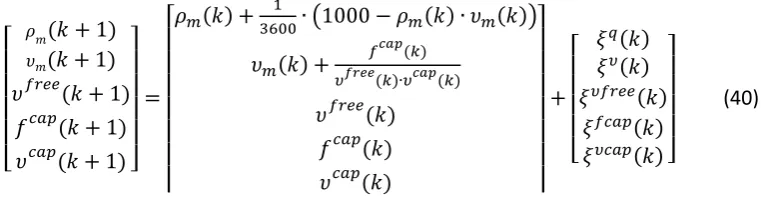
4.9.1. Network consisting of one link and fundamental diagram parameters estimation

For the first numerical example, we consider a network that consists of only one link, as shown in Figure 6. The link consists of one lane and its length is 1 km. For this link, a fixed inflow is considered, with a value of 𝑞𝑖𝑛=1000 veh/h. The time step of the simulation is set to 1 second.

The full state vector in this example contains the density (𝜌𝑚) and speed (𝜐𝑚) of the link, as

well as the fundamental diagram parameters (𝑣𝑓𝑟𝑒𝑒, 𝑓𝑐𝑎𝑝 and 𝜐𝑐𝑎𝑝). Therefore, the full state vector is the following:

(35)

[image:35.595.124.508.389.490.2]

23

Figure 6. Network consisting of one link.

The density propagation equation is based on (14), after replacing the values for the duration of the time step 𝑇, number of lanes 𝜆 and length of the link 𝐿, as well as the term

𝜌𝑖−1(𝑘) ∙ 𝜐𝑖−1(𝑘) ∙ 𝜆𝑖−1 with 1000, which is the value of 𝑞𝑖𝑛:

𝜌𝑚(𝑘 + 1) = 𝜌𝑚(𝑘) + 1

3600∙ (1000 − 𝜌𝑚(𝑘) ∙ 𝜐𝑚(𝑘)) + 𝜉

𝑞_(𝑘) ₍₃₈₎

In order to avoid complex equations in this example, a much simpler speed equation is used, which has been randomly setup, simply making sure that it contains all fundamental diagram parameters in it:

𝜐𝑚(𝑘 + 1) = 𝜐𝑚(𝑘) + 𝑓𝑐𝑎𝑝

𝜐𝑓𝑟𝑒𝑒∙𝜐𝑐𝑎𝑝 + 𝜉

𝜐_(𝑘) ₍₃₉₎

Therefore, the full state transition model can be described as:

[

𝜌_𝑚(𝑘 + 1)

𝜐𝑚(𝑘 + 1)

𝜐𝑓𝑟𝑒𝑒(𝑘 + 1) 𝑓𝑐𝑎𝑝(𝑘 + 1) 𝜐𝑐𝑎𝑝(𝑘 + 1) ]

=

𝜌𝑚(𝑘) + 1

3600∙ (1000 − 𝜌𝑚(𝑘) ∙ 𝜐𝑚(𝑘))

𝜐𝑚(𝑘) +

𝑓𝑐𝑎𝑝(𝑘)

𝜐𝑓𝑟𝑒𝑒(𝑘)∙𝜐𝑐𝑎𝑝(𝑘)

𝜐𝑓𝑟𝑒𝑒(𝑘) 𝑓𝑐𝑎𝑝(𝑘) 𝜐𝑐𝑎𝑝(𝑘)

+

[

𝜉𝑞(𝑘) 𝜉𝜐(𝑘) 𝜉𝜐𝑓𝑟𝑒𝑒(𝑘)

𝜉𝑓𝑐𝑎𝑝(𝑘) 𝜉𝜐𝑐𝑎𝑝(𝑘) ]

(40)

The Jacobian 𝐹 with respect to the state 𝑥 of the state transition function 𝑓 is a 5x5 matrix:

𝐹 =

1 − 𝜐𝑚 3600 −

𝜌𝑚

3600 0 0 0

0 1 − 𝑓

𝑐𝑎𝑝

(𝜐𝑓𝑟𝑒𝑒)2_{∙ 𝜐}𝑐𝑎𝑝

1

𝜐𝑓𝑟𝑒𝑒∙ 𝜐𝑐𝑎𝑝 −

𝑓𝑐𝑎𝑝 (𝜐𝑐𝑎𝑝)2_{∙ 𝜐}𝑓𝑟𝑒𝑒

0 0 1 0 0

0 0 0 1 0

0 0 0 0 1

(41)

The relevant measurement functions for the speed and flow are the following:

ℎ𝑣𝑚(𝑘) = 𝑣𝑚(𝑘) + 𝛾𝑚

𝜐_(𝑘) ₍₄₂₎

ℎ_𝑞

𝑚(𝑘) = 𝜌𝑚(𝑘) ∙ 𝜐𝑚(𝑘) + 𝜉

𝑞_{(𝑘) + 𝛾} 𝑚

𝑞

(36)

24 The Jacobians of the measurement functions are the following:

𝐻𝑣= (0, 1, 0, 0, 0) (44)

𝐻𝑞= (𝑣𝑚, 𝜌𝑚, 0, 0, 0) (45)

The standard deviations for the uncertainties of the process and the measurements are set to 𝜉𝑞 = 𝜉𝜐= 𝛾𝑚𝜐 = 𝛾𝑚𝑞 = 0.25 and for the uncertainties of the fundamental diagram

parameters to 𝜉𝜐𝑓𝑟𝑒𝑒= 𝜉𝑓𝑐𝑎𝑝= 𝜉𝜐𝑐𝑎𝑝 = 1.

The process noise covariance matrix 𝑇 = diag(𝜉𝑞, 𝜉𝜐, 𝜉𝜐𝑓𝑟𝑒𝑒, 𝜉𝑓𝑐𝑎𝑝, 𝜉𝜐𝑐𝑎𝑝) = = diag(0.25, 0.25, 1, 1, 1).

The EKF is initialized with the following settings: Initial state: 𝑥(0) = (19.9, 50, 49, 1610, 34) T

Initial covariance matrix 𝛴(0) = diag(1)

The example measurements that will be used for the first time step are the following:

𝑧𝑞(1) = 1020 and 𝑧𝜐(1) = 48.

Prediction step

The state estimate propagation for the first time step 𝑥̂(1) is given by (40), by replacing the values of the initial state 𝑥(0). The resulting state is:

𝑥̂(1) = (19.9014, 50.9664, 49, 1610, 34) T_.

The Jacobian 𝐹 calculated at 𝑥̂(1) is calculated from (41):

𝐹 =

0.9858 −0.0055 0 0 0

0 1 −0.0197 0.0006 −0.0284

0 0 1 0 0

0 0 0 1 0

0 0 0 0 1

The error covariance propagation (𝛴) is given by (32):

𝛴 =

1.2219 −0.0055 0 0 0

-0.0055 1 −0.0197 0.0006 −0.0284

0 −0.0197 2 0 0

0 0.0006 0 2 0

(37)

25 Correction step

The application of the correction step must be repeated twice, as there are measurements of both the speed and the flow of the link.

Starting with the flow measurement, the process begins with the prediction of the measurement from the measurement functions:

𝑧̂𝑞(1) = 𝜌𝑚(1) ∙ 𝜐𝑚(1) = 19.9014⁡ ∙ 50.9664 = 1014.3⁡veh/h

The Jacobian of the flow measurement function from (45) is:

𝐻𝑞 = (𝑣𝑚, 𝜌𝑚, 0, 0, 0) = (50.9664, 19.9014, 0, 0, 0)

The Kalman gain is calculated from (34):

𝐾 = [0.0170, 0.0067, -0,0001, 0.000003, -0.000155]T

The state estimate update is calculated from (35):

𝑥̂(1) = [19.9982, 51.0047, 48.9994, 1610.00002, 33.9991] T

The error covariance matrix 𝛴 is calculated from (36):

𝛴 =

0.1657 −0.4238 0.0067 -0.000203 0.0096

-0.4238 1.0855 −0.0171 0.00052 −0.0246

0.0067 −0.0171 2 0.0000013 -0.0000607

-0.000203 0.00052 0.0000013 2 0.00000185

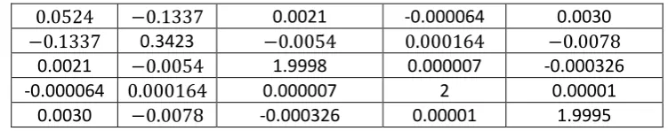
0.0096 −0.0284 -0.0000607 0.00000185 1.9999

The same process is repeated for the fusion of the speed measurements, using the above new values for the 𝑥̂(1) and 𝛴 after fusion of the flow measurement:

𝑧̂𝜐(1) = 𝜐𝑚(1) = 51.0047⁡𝑘𝑚/h

𝐻𝑣= (0, 1, 0, 0, 0)

𝐾 = [-0.2673, 0.68465, -0.010773, 0.000328, -0.015526]T

(38)

26

𝛴 =

0.0524 −0.1337 0.0021 -0.000064 0.0030

−0.1337 0.3423 −0.0054 0.000164 −0.0078

0.0021 −0.0054 1.9998 0.000007 -0.000326

-0.000064 0.000164 0.000007 2 0.00001

0.0030 −0.0078 -0.000326 0.00001 1.9995

After fusing all measurements, the resulting value of 𝑥̂is the “a posteriori” estimate of the

traffic state, the corrected state for the first time step. This value of the state and the resulting value of 𝛴 are used as the respective initial values for the next time step.

Therefore, the values 𝑥(1) = 𝑥̂(1) = [20.8014, 48.9475, 49.032, 1609.99903, 34.046] T_and

𝛴(1) = 𝛴 are the corrected state for the first time step. The process continues with the next time step, where these values are used for the “a priori” state estimate of the second time step.

4.9.2. Network consisting of two links, no fundamental diagram parameters estimation

For the second numerical example, we consider a network consisting of two links, as shown in Figure 7. The links consist of one lane and their length is 1 km each. For the first link, a fixed inflow is considered, with a value of 𝑞𝑖𝑛=1000 veh/h. The time step of the simulation is set to 1 second. In this example we omit the fundamental diagram parameters and use a simpler speed equation for simplicity reasons.

The full state vector in this example contains the densities (𝜌1 and 𝜌2) and speeds (𝜐1 and

𝜐2) of the links. Therefore, the full state vector is the following:

𝑥 = (𝜌1, 𝜐1, 𝜌2, 𝜐2) (46)

The density propagation equations are based on (14), after replacing the values for the duration of the time step 𝑇, number of lanes 𝜆 and length of the link 𝐿, as well as the term

𝜌𝑖−1(𝑘) ∙ 𝜐𝑖−1(𝑘) ∙ 𝜆𝑖−1 with 1000, which is the value of 𝑞𝑖𝑛 for the first link:

𝜌1(𝑘 + 1) = 𝜌1(𝑘) + 1

3600∙ (1000 − 𝜌1(𝑘) ∙ 𝜐1(𝑘)) + 𝜉

𝑞_(𝑘) ₍₄₇₎

𝜌2(𝑘 + 1) = 𝜌2(𝑘) + 1

3600∙ (𝜌1(𝑘) ∙ 𝜐1(𝑘) − 𝜌2(𝑘) ∙ 𝜐2(𝑘)) + 𝜉

[image:38.595.108.484.99.173.2]

𝑞_(𝑘) ₍₄₈₎

(39)

27 In order to avoid complex equations in this example, too, a simpler speed equation is used, keeping only the convection term. For the first link, a constant upstream speed of 50 km/h is assumed:

𝜐1(𝑘 + 1) = 𝜐1(𝑘) + 1

3600∙ 𝜐1(𝑘) ∙ (50 − 𝜐1(𝑘)) + 𝜉

𝜐_(𝑘) ₍₄₉₎

𝜐2(𝑘 + 1) = 𝜐2(𝑘) + 1

3600∙ 𝜐2(𝑘) ∙ (𝜐1(𝑘) − 𝜐2(𝑘)) + 𝜉

𝜐_(𝑘) ₍₅₀₎

Therefore, the full state transition model can be described as:

[

𝜌₁(𝑘 + 1)

𝜐1(𝑘 + 1) 𝜌₂(𝑘 + 1)

𝜐2(𝑘 + 1)

] =

𝜌1(𝑘) + 1

3600∙ (1000 − 𝜌1(𝑘) ∙ 𝜐1(𝑘))

𝜐1(𝑘) + 1

3600∙ 𝜐1(𝑘) ∙ (50 − 𝜐1(𝑘))

𝜌2(𝑘) + 1

3600∙ (𝜌1(𝑘) ∙ 𝜐1(𝑘) − 𝜌2(𝑘) ∙ 𝜐2(𝑘))

𝜌2(𝑘) + 1

3600∙ (𝜌1(𝑘) ∙ 𝜐1(𝑘) − 𝜌2(𝑘) ∙ 𝜐2(𝑘))

+

[ 𝜉𝑞_(𝑘)

𝜉𝜐(𝑘) 𝜉𝑞(𝑘) 𝜉𝜐(𝑘) ]

(51)

The Jacobian 𝐹 with respect to the state 𝑥 of the state transition function 𝑓 is a 4x4 matrix:

𝐹 =

1 − 𝜐1

3600 − 𝜌1

3600 0 0

0 1.0139 - 𝜐1

3600 0 0

𝜐₁ 3600

𝜌1

3600 1 − 𝜐2

3600 − 𝜌2

3600

0 𝜐2

3600 0

𝜐1

3600− 𝜐2

1800+ 1

(52)

The relevant measurement functions for the speed and flow are the following:

ℎ𝑣1(𝑘) = 𝑣1(𝑘) + 𝛾 𝜐_(𝑘)

(53)

ℎ𝑣2(𝑘) = 𝑣2(𝑘) + 𝛾

𝜐_(𝑘) ₍₅₄₎

ℎ_𝑞

1(𝑘) = 𝜌1(𝑘) ∙ 𝜐1(𝑘) + 𝜉

𝑞_{(𝑘) + 𝛾}𝑞

(𝑘) (55)

ℎ_𝑞

2(𝑘) = 𝜌2(𝑘) ∙ 𝜐2(𝑘) + 𝜉

𝑞_{(𝑘) + 𝛾}𝑞

(𝑘) (56)

The Jacobians of the measurement functions are the following:

𝐻𝑣1= (0, 1, 0, 0) (57)

𝐻𝑣2= (0, 0, 0, 1) (58)

𝐻𝑞1= (𝑣1, 𝜌1, 0, 0) (59)

𝐻𝑞2= (0,0, 𝑣2, 𝜌2) (60)

A model based approach for state estimation for networks