Permission based separation logic for Scala

Master's Thesis

Author:

Charl de Leur

Graduation Comittee: prof. dr. M. Huisman

dr. S.C.C. Blom dr. J. Kuper

full compatibility with existingJavalibraries and code, while providing a multitude of advanced features compared toJavaitself.

Permission-based separation logichas proven to be a powerful formalism in reasoning about memory and concurrency

in object-oriented programs – specifically inJava, but there are still challenges in reasoning about more advanced languages such asScala.

1 Introduction 3

1.1 Motivation . . . 3

1.2 Contribution . . . 3

1.3 Document Outline . . . 3

2 Background Information & Previous Work 5 2.1 Static Contract Analysis . . . 5

2.2 Verification using Classic Program Logic . . . 5

2.3 Separation Logic . . . 7

2.4 Formal Semantics . . . 13

3 TheScalaProgramming Language 15 3.1 Introduction . . . 15

3.2 A Guided Tour ofScala . . . 15

4 A Model Language Based onScala 22 4.1 Introduction . . . 22

4.2 Program Contexts & Zippers . . . 22

4.3 Scala Corewith only Basic Expressions . . . 27

4.4 ExtendingScala Corewith Functions . . . 34

4.5 ExtendingScala Corewith Exceptions . . . 43

4.6 ExtendingScala Corewith Classes & Traits . . . 47

4.7 ExtendingScala Corewith Threads & Locking . . . 57

4.8 Comparisons . . . 64

5 Adapting Permission-Based Separation Logic toScala 66 5.1 Introduction . . . 66

5.2 Elements of our Separation Logic . . . 66

5.3 TypingScala Corewith Basic Expressions & Functions . . . 72

5.4 Separation Logic for Scala Corewith Basic Expressions & Functions . . . 76

5.5 ExpandingSeparation Logic for Scala Coreto Exceptions . . . 84

5.6 ExpandingSeparation Logic for Scala Coreto Classes & Traits . . . 85

5.7 ExpandingSeparation Logic for Scala Corewith Permissions . . . 88

5.8 Related Work . . . 88

6 Specification ofScalaActors: A Case Study 90 6.1 Introduction . . . 90

6.2 On The Actor Model . . . 90

6.3 UsingScalaActors . . . 91

6.4 Architecture ofScalaActors . . . 97

6.5 Implementation and Specification ofScalaActors . . . 98

6.6 Conclusions . . . 128

7 Conclusions & Future Work 129 7.1 Summary . . . 129

7.2 Contribution . . . 129

1 Introduction

1.1 Motivation

The recent years have seen the growing popularity of language features, being borrowed from different paradigms such as functional programming, added to imperative and object-oriented languages to create hybrid paradigm languages. Popular examples include the inclusion of first-class functions in languages such asC

#

Meanwhile the recent years have also seen the rise of multi-threading and concurrency as a means to quench the ever-increasing thirst for computing power. With this new focus on concurrency, also came a response from the proponents of formal methods in computer science, with model checking and concurrent program verification techniques allowing for a more reliable creation of concurrent programs. This is important, as writing these concurrent programs by hand, without formal techniques, proved error-prone.

In this thesis we examine concurrent program verification techniques – especially the use of separation logic – in how they manage with a multi-paradigm language such asScala. We do so by first examing the current state of the art in program verification using separation logic and examining theScalalanguage itself. We will then start a formalization process in which we develop a formal semantics for an interesting subset ofScalawith an accompanying separation logic to prove its correctness. Finally we will provide a case study in which we use our logic to provide a specification of theScalaactor concurrency library.

1.2 Contribution

Our contribution is a means to specifyScalaprograms using permission-based separation logic, with a focus on a concise and correct method to specify first-class functions and lexical closures and a case study, which demonstrates our approach and its viability. We will provide a formalization of a subset ofScalaincluding lexical closures and exceptions. Using this formalized subset, we will establish type-safety and a separation logic to establish memory safety and race freedom.

1.3 Document Outline

Background (Section 2)

In theBackgroundsection, we start with an introduction to, and background of, formal program verification using, first, Hoare logic and following that, Separation Logic. We show the defining features of separation logic and their advantages and uses in the verification of shared memory languages and concurrency. Secondly, we have a look at formal semantics, their uses and their role in program verification, by giving a short overview of the three most common forms of formalizing semantics, beingaxiomatic,operationalanddenotationalformalization.

TheScalaLanguage (Section 3)

A Formalized Model Language forScala(Section 4)

An essential part of program verification, is the formalization of the semantics of the language being verified. AsScala is a multi-paradigm language with too many features to cover in this work, we define a number of subsets: We start with a basic expression language, which we first expand with first-class functions and closures, then with exceptions, classes and finally multi-threading. These subsets ofScalaare then consecutively formalized using a program-context approach, resulting in what we callScala Core.

Separation Logic forScala Core(Section 5)

The primary goal in this section is to provide a variant of separation logic which can be used to verify programs written in our model language, secondly we provide typing rules, to assure type-safety. We start with the basic expression language with functions, as this is one of the most interesting cases for verification and continue towards exceptions and multi-threading.

A Case Study (Section 6)

With our formalization complete, it is interesting to see how it would function when used to specify a real-world larger piece of software. In this section we do so by writing a specification for theScalaactor library, which is as an alternative to shared-memory concurrency.

Conclusions and Future Work (Section 7)

2 Background Information & Previous Work

For the work presented in this thesis, we build on previous work in the verification of (concurrent) programs, specifically via the use of separation logic and on the work in formal semantics. In this section we shall expand on the existing work in these areas, with a focus on theJVMand onScalain particular. We shall start with a general introduction to static contract analysis in Section 2.1 and program logics in Section 2.2 and proceed with an introduction to separation logic in Section 2.3.1, which we shall expand toConcurrent Separation Logicin Section 2.3. Finally we shall give an introduction to formal semantics in Section 2.4

2.1 Static Contract Analysis

Of all the recent formal methods for program analysis, such as software model checking [54], static analysis [42, 41] and interactive theorem proving [33], our focus will be on program verification using logic assertions in program code, as first suggested by Hoare [29]. These assertions form contracts [39] between computational modules in software from which proof obligations can be derived and solved. This analysis can be done without executing the application, making it static in nature. Well-known tools based on this formalism include the more academic toolsEsc/Java[24] andSpec

#

#

2.2 Verification using Classic Program Logic

2.2.1 Properties of Code

sort(a : Int[]) : Int[] {

... }

Listing 1:Simple Sort

We shall illustrate properties of code, using Listing 1, which shows a simple method, that sorts a given array. We can, independently of the implementation, state that this method indeed sorts an array, in first-order logic – e.g. as ∀𝑖, 𝑗.0 ≤ 𝑖 < 𝑗 < 𝑎.𝑙𝑒𝑛𝑔𝑡ℎ ⇒ 𝑎[𝑖] ≤ 𝑎[𝑗]. Unfortunately, there is no practical means to tell where this property holds: It could just as well have been a requirement for the method to execute, instead of a condition on the result. The solution, as pioneered by Hoare, involves making location explicit, by dividing the properties in so-called preconditions and postconditions [29]:

• Precondition: A property that should hold at method entry, specifying what is required to deliver correct output.

• Postcondition: A property that should hold at method exit, specifying what the method guarantees to the caller.

With these, we can now speak of what are commonly referred to asHoare triples: Triples in the form of{𝑃}𝐶{𝑄}, where𝑃is a precondition,𝐶is a statement and𝑄is a postcondition. the triple is defined as having the following interpretation:

• Definition:Given that𝑃is satisfied in a state𝑠, and𝐶terminates in state𝑠′, then𝑄is satisfied in state𝑠′.

We can now specify a Hoare triple for the example in Listing 1 – in Listing 2:

// {𝑡𝑟𝑢𝑒}

sort(a : Array[Int]) : Array[Int] {

/* […] */

}

// {∀ 𝑖, 𝑗. 0 ≤ 𝑖 < 𝑗 < 𝑙𝑒𝑛𝑔𝑡ℎ(𝑎) ⇒ 𝑎[𝑖] ≤ 𝑎[𝑗]}

Listing 2:Simple Sort with Hoare Triple

2.2.2 Reasoning about Properties

Once we have a Hoare triple for a method – also called a proof outline – the next step is to reason about them and establish their validity. This is done by applying the axioms and logic rules ofHoare logicto determine a truth value [29]. A simple example of an axiom being the empty statement axiom, which states that any preconditions holding before theskip-statement will hold after – essentially saying thatskiphas no impact on the program state – is shown in Fig. 1:

𝑆𝑘𝑖𝑝

{𝑃}𝑠𝑘𝑖𝑝{𝑃}

Figure 1:The Skip Axiom

An example of a rule is the sequential composition rule – shown in Fig. 2 – which specifies the conditions that should hold for sequential statements:

{𝑃}𝑆1{𝑄} {𝑄}𝑆2{𝑅} 𝑆𝑒𝑞

{𝑃}𝑆1; 𝑆2{𝑅}

Figure 2:The Seq Rule

Given these examples, proving correctness of a program would seem like a lot of work, and indeed, these correctness proofs tend to take up sheets and sheets with rules being applied over and over until finally axiomatic statements are reached. Fortunately, this part can be largely (but not entirely) automated [24], resulting in the proof outline being sufficient to automatically determine correctness. This provides the basis for the practical use of formal verification via program logics. One essentially provides proof outlines and lets the automatic reasoning tool determine whether they hold; this type of verification is often referred to as static checking.

2.2.3 Relation to Programming by Contract

The pre- and postconditions mentioned in Section 2.2.1 may sound familiar to anyone familiar with the concept of design by contract (DBC); and indeed, the specifications are similar. In practice, in DBC, the specifications are often defined as a part of the programming language itself and thus executable [38]. The contracts are compiled to executable code along with the program code and thus violations of the contract are prohibited at runtime. This also means that DBC by itself makes no guarantees, without executing the program (of which the specification is now part). Because of this, it is often referred to as runtime checking, as opposed to the static checking mentioned in Section 2.2.2.

theJMLlanguage as specifications to provide static checking and runtime checking respectively, andCode Contracts, which provides runtime as well as static checking on the same specifications.

2.2.4 Limitations of the Classic Approach

So far it seems that classic program logics are quite powerful in reasoning about programs, to the point that static checking of advanced specification languages such asJMLcan be built on top of them. However, there are limitations in the classical approach, mostly concerned with reasoning about pointers and memory:

Assignment Axiom {𝑃[𝐸/𝑥]}𝑥 ∶= 𝐸{𝑃}

Assignment with values {𝑦 + 7 > 42}𝑥 ∶= 𝑦 + 7{𝑥 > 42}

Assignment with pointers {𝑦.𝑎 = 42}𝑥.𝑎 ∶= 7{𝑦.𝑎 = 42}

Figure 3:The Issue with Pointers

To illustrate the pointer issue, Fig. 3 shows an example of the assignment axiom in use, which states that if𝑃holds and all occurences of the assigned expression𝐸in𝑃are replaced by the variable𝑥,𝑃should still hold. For the example with values this clearly holds and for the example with pointers it seems to hold, but this turns out to be unsound when𝑥aliases𝑦, thus invalidating the axiom for use with pointers.

[𝑦 ∶= −𝑦; 𝑥 ∶= 𝑥 + 1; 𝑦 ∶= −𝑦] (1)

[𝑥 ∶= 𝑥 + 1] (2)

Figure 4:The Issue with Concurrency

Figure 4 shows two cases which in sequential execution satisfy the same input and output conditions, but in concurrent execution act differently due to interference with other statements of the first case. This means classic Hoare logic provides no guarantees of race-freedom. The result of this is that classic program logics are unsuitable to reason about concurrent programs, as any assertion established in a thread, can possibly be invalidated by another thread, at any time during the execution. While there exist logics which can take into account these multi-threaded scenarios, they tend to be either – in the case ofOwicki-Gries[46] andRely-guarantee[36] – too general to be of practical use, or – in the case ofconcurrent Hoare logics[30], too simplistic to handle the complex situations, involving heaps, in modern programming languages.

To allow for reasoning with concurrency and pointers, we must then look at a logic which can properly reason about memory; enter Separation logic (SL).

2.3 Separation Logic

2.3.1 Sequential Separation Logic

locations to values (representing objects or otherwise dynamically allocated memory). These additions allow us to make judgements of the form𝑠, ℎ ⊨ 𝑃, where𝑠is a store,𝑝a heap and𝑃an assertion about them.

To allow for concise definitions of assertions over the heap and store, classical separation logic extends first-order logic with four assertions:

⟨𝑎𝑠𝑠𝑒𝑟𝑡⟩ ∶∶ = ⋯

∣emp empty heap

∣ ⟨𝑒𝑥𝑝⟩ ↦ ⟨𝑒𝑥𝑝⟩ singleton heap

∣ ⟨𝑎𝑠𝑠𝑒𝑟𝑡⟩ ∗ ⟨𝑎𝑠𝑠𝑒𝑟𝑡⟩ separating conjunction

∣ ⟨𝑎𝑠𝑠𝑒𝑟𝑡⟩ ∗ ⟨𝑎𝑠𝑠𝑒𝑟𝑡⟩ separating implication

Figure 5:Extensions to First-Order Logic

• Theemppredicate denotes the empty heap and acts as the unit element for separation logic operations.

• The points-to predicate𝑒 ↦ 𝑒′means that the location𝑒maps to value𝑒′.

• The resource (or separating) conjunction𝜙 ∗ 𝜓means that the heapℎcan be split up in 2 disjoint partsℎ1⊥ℎ2

where𝑠, ℎ1⊨ 𝜙, and𝑠, ℎ2⊨ 𝜓.

• 𝜙 ∗ 𝜓asserts that, if the current heap is extended with a disjoint part in which𝜙holds, then𝜓will hold in the extended heap.

However, we will mostly be dealing with al alternate variant, called intuitionistic separation logic[21, 47], which, instead of extending classic first-order logic, extends intuitionistic logic. This is as classical separation logic is based on reasoning about the entire heap, which presents issues with garbage collected language likeScala, where the heap is in a state of flux and cannot generally be completely specified. The intuitionistic variant therefore admits weakening, that is to say𝑃 ∗ 𝑄 ⇒ 𝑄. Normally this would allow for memory leaks, but the garbage collection takes care of this. Instead of usingempas the unit element, intuitinionistic separation logic drops this predicate and usestrue.

𝑒 ↦ 𝑒1, … , 𝑒𝑛 𝑑𝑒𝑓

= 𝑒 ↦ 𝑒1∗ … ∗ 𝑒 + (𝑛 − 1) ↦ 𝑒𝑛

𝑝 = 𝑥 ↦ 3 𝑟 = 𝑥 ↦ 3, 𝑦

𝑞 = 𝑦 ↦ 3 𝑠 = 𝑦 ↦ 3, 𝑥

𝑝 ∗ 𝑞

Figure 6:Example Assertions in Separation Logic

Given this syntax, we will now visualize the examples given in Fig. 6:

• 𝑝asserts that𝑥maps to a cell containing 3.

𝑥 3

• 𝑝 ∗ 𝑞asserts that𝑝and𝑞hold in disjoint parts of the heap.

𝑥 ₃ 𝑦 ₃

• 𝑟 ∗ 𝑠asserts that two adjacent pairs hold in disjoint heaps.

• 𝑟 ∧ 𝑠asserts that two adjacent pairs hold in the same heap.

𝑥, 𝑦 3

• 𝑝 ∗ 𝑞asserts that, if the current heap is extended with a disjoint part in which𝑝holds, then𝑞will hold in the extended heap.

ℎ1 ℎ1

ℎ2 ℎ1∗ ℎ2

𝑝

ℎ1 𝑞

Now let us look at an example specification of a simpleScala-method, withPointsTobeing the ASCII representation of↦:

class Simple {

var x = 0 var y = 1 var z = 3

/*@

requires PointsTo(x, _) ensures PointsTo(x, \result)

*/

def inc() : Int {

x = x+1

x

} }

Listing 3:A Simple Specification in Separation Logic

The exact meaning of the specification in Listing 3 is not yet relevant, but an important detail to note is that the specification only mentions the part of the heap relevant to the method, in this case𝑥. This is called local reasoning, made possible by the frame rule – shown in Fig. 7 – which prevents us from repeatedly having to specify the entire heap.

{𝑃}𝑆{𝑄}

𝐹𝑟𝑎𝑚𝑒 None of the variables modified in𝑆occur free in𝑅

{𝑃 ∗ 𝑅}𝑆{𝑄 ∗ 𝑅}

Figure 7:The Frame Rule

state, satisfying𝑃 ∗ 𝑅, and that its execution will not alter the expanded part of the state i.e. the heap – outside of what is locally relevant – does not need to be considered when writing specifications.

2.3.2 Abstract Predicates

A practical extension to separation logic, especially for verification of data structures, isabstract predicates[48]. Similarly to abstract data types in programming languages, abstract predicates add abstraction to the logical frame-work.

Abstract predicates consist of a name and a formula and arescoped:

• Verified code inside the scope can use both the predicate’s name and body.

• Verified code outside the scope must treat the predicate atomically.

• Free variables in the body should be contained in the arguments to the predicate.

To illustrate the use of abstract predicates for data abstraction, Fig. 8 shows the abstraction for singly-linked lists which is defined by induction on the length of the sequence𝛼. The𝐥𝐢𝐬𝐭predicate takes a sequence and a pointer to the first element as its arguments; An empty list consists of an empty sequence and a pointer to𝐧𝐢𝐥and longer lists are inductively defined by a pointer to a first element and the assertion that the following sequence is once again a list.

𝐥𝐢𝐬𝐭 𝜖 𝑖𝑑𝑒𝑓= 𝐞𝐦𝐩 ∧ 𝑖 ↦ 𝐧𝐢𝐥

𝐥𝐢𝐬𝐭 𝑎 ∶ 𝛼 𝑖𝑑𝑒𝑓= ∃𝑗.𝑖 ↦ 𝑎, 𝑗 ∗ 𝐥𝐢𝐬𝐭 𝛼𝑗

Figure 8:A List Abstraction using Abstract Predicates

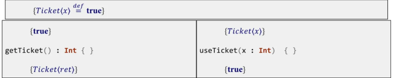
Figure 9 shows another example of abstract predicates, but one where a predicate functions more like a access ticket.

{𝑇𝑖𝑐𝑘𝑒𝑡⟨𝑥⟩𝑑𝑒𝑓= true}

{true}

getTicket() : Int { }

{𝑇𝑖𝑐𝑘𝑒𝑡⟨𝑟𝑒𝑡⟩}

{𝑇𝑖𝑐𝑘𝑒𝑡⟨𝑥⟩}

useTicket(x : Int) { }

{true}

Figure 9:An Example use of Abstract Predicates

2.3.3 Fractional Permissions

We shall illustrate this with an example in Listing 4:

class Simple {

var x = 0

/*@

requires PointsTo(x, 1, _) ensures PointsTo(x, \result)

*/

def inc() : Int {

x = x+1

x

}

/*@

requires PointsTo(x, 1/2, _) ensures PointsTo(x, 1/2, _)

*/

def read() : Int {

x

} }

Listing 4:A Simple Example of Permissions

In Listing 4inc()requires a permission of1, andread()one of1₂, so at most two threads are allowed to readxusing

read(), but only one is ever allowed to increment, at a time.

When considering resources and permissions, the magic wand gains another use in the trading of permissions: Given a heap in which𝑝 ∗ 𝑞holds, the resource𝑝can be consumed, yielding the resource𝑞. This use is visualized in Fig. 10.

• 𝑟 = (𝑥0.3↦ 9) ∗ (𝑥↦ 9)1 holds inℎ1.

ℎ1=𝑥 9

0.7

• Heap extension happens as before, but permissions are combined.

𝑥 0.3 + 0.7 9

• Given the resource needed, we can trade:((𝑥0.3↦ 9) ∗ 𝑟) ⇒ (𝑥↦ 9)1

ℎ1=𝑥 9

1

• (𝑥0.3↦ 9)is consumed in the trade.

2.3.4 Locks

Another key addition we require, is a means to reason about locks and reentrancy. Fortunately, a solution [28, 5] exists:

First we defineinv, the so-called resource invariant, describing the resources a lock protects e.g. in Listing 5 the resource invariant protects𝑥.

class Simple {

/*@ inv = PointsTo(x, 1 _) */

var x = 0 /*@ commit */

/*@

requires Lockset(S) * (S contains this -* inv) * initialized

ensures Lockset(S) * (S contains this -* inv)

*/

def inc() : Int {

synchronized

{

x+=1

x

} } }

Listing 5:Specification of a Lock in Separation Logic

Asinvmay require initialization before becoming invariant, the invariant starts in a suspended state. Only when we commit the invariant, it is actually required to invariantly hold. A common place for such a commit to happen would be at the end of a constructor as in Listing 5.

Secondly we extend the logic with the following predicates:

• 𝐿𝑜𝑐𝑘𝑠𝑒𝑡(𝑆): The multiset of locks held by the current thread.𝐿𝑜𝑐𝑘𝑠𝑒𝑡(𝑆)is empty on creation of a new thread.

• 𝑒.𝑓𝑟𝑒𝑠ℎ: The resource invariant of𝑒is not yet initialized en therefore doesn’t hold.

• 𝑒.𝑖𝑛𝑖𝑡𝑖𝑎𝑙𝑖𝑧𝑒𝑑: The resource invariant of𝑒can be safely assumed to hold.

• 𝑆 𝑐𝑜𝑛𝑡𝑎𝑖𝑛𝑠 𝑒: The multiset of locks of the current thread contains the lock𝑒.

We will require an addition to the rule for object creation, regardless of the actual specifics of the existing rule, that specifies that all new objects (and therefore locks) are fresh. Furthermore, we require the additional rules given in Fig. 11:

• Thelockrule applies for a lock that is acquired non-reentrantly. The precondition specifies this stating there is a lockset𝑆for this thread, but the lock is not part of it. Furthermore the lock is required to have an initialized resource invariant. In the postcondition the lock must have been added to the lockset.

• Therelockrule is a simple variant oflock, for the reentrant case.

• Finally we have thecommitrule, which promotes a fresh lock to an initialized one.

In the rules given we assume, for easier illustration, a language with dedicatedlockandunlockprimitives, but this is extendable to constructions likesynchronizedandwait/notify.

Lock

{Lockset(S) * ¬(S contains u) * u.initialized} {lock(u)}

{Lockset(u.S) * u.inv} Relock

{Lockset(u.S)} {lock(u)} {Lockset(u.u.S)} Unlock _{{Lockset(u.S) * u.inv}}

{unlock(u)} {Lockset(S)} Commit

{Lockset(S) * u.fresh} {u.commit}

{Lockset(S) * ¬(S contains u) * u.initialized}

Figure 11:Extra Rules to Deal with Locks

2.4 Formal Semantics

As previously stated in Section 1, one of our goals is to provide a formal semantics forScala; Here we shall give an introduction to formal semantics and its relevance to this thesis.

Programming languages are generally specified informally, using a language specification document, such as the ones forJava[27] andScala[43], but to reason about languages using the previously covered program logics, this is insufficient; For them languages need to have a strict mathematical meaning, which can be linked to and used in the logical formulas. Such a mathematical description of language meaning is called a formal program semantics.

The idea of program semantics was introduced by Floyd [25] and formal semantics now exist in three major categories, namely axiomatic semantics, operational semantics and denotational semantics. For our purposes, we will mainly be interested in operational semantics, for the language itself, and, to a lesser extent, in axiomatic semantics and denotational semantics, to define the meaning of the assertion logic and its relation to the language semantics.

Operational semantics describe what is valid in a language as sequences of computational steps. They do so either – in the case of big-step semantics – by describing the overall result of an execution [34] or – in the case of small-step semantics – by describing the individual steps of the computation [50], using rules. Because our work is focused on concurrency, we will be dealing with the latter. We shall give a small example of a small-step semantics of a toy language:

𝑒 ∶∶= 𝑚 ∣ 𝑒0+ 𝑒1

Figure 12:A Very Simple Language

Our demonstration language will consist of expressions, which can be either be a constant or an addition between two expressions. These expressions can be evaluated in four steps:

• Constants

• Addition

1. In𝑒0+ 𝑒1,𝑒0is evaluated to a constant, say𝑚0.

2. In𝑒0+ 𝑒1,𝑒1is evaluated to a constant, say𝑚1.

3. In𝑒0+ 𝑒1,𝑚0+ 𝑚1is evaluated to a constant, say𝑚2.

These steps can now be formalized as rules, which take the form premises conclusion:

𝑒0→ 𝑒0′ 𝑒0+ 𝑒1→ 𝑒0′+ 𝑒1

𝑒1→ 𝑒1′ 𝑚0+ 𝑒1→ 𝑚0+ 𝑒1′

With𝑚2the sum of𝑚0and𝑚1.

𝑚0+ 𝑚1→ 𝑚2

Figure 13:Reduction Rules for the Very Simple Language

These rules now give a strict formal meaning to our simple language.

Axiomatic semantics describe meaning using rules and axioms, of which we have seen examples in Section 2.3.

3 The

Scala

Programming Language

3.1 Introduction

Scala1[22] is a purely object-oriented language with a unified type-system, blending in functional concepts, imple-mented as a statically typed language on theJVM2, seamlessly interoperating with the existing Java libraries [44, pp. 49, 55–58]. Notable Features ofScalainclude:

• First-class functions and lexical closures.

• Traits.

• Unified Type System.

• Case Classes.

• Singleton Objects.

• Pattern Matching.

• Limited Type Inference.

• Properties.

• Abstract Types.

As the work presented in this document depends on an understanding of theScalalanguage, we will take some time to mention and clarify some of the features used. We will assume an understanding of theJavalanguage andJVM, as well as a basic understanding of functional programming and languages. Furthermore, this is not meant to be a full tutorial onScala, as better resources for that exist elsewhere [44]. We shall illustrate the features of the language using the sample program given in Listing 7.

3.2 A Guided Tour of

Scala

The program described in Listing 7 represents and evaluates simple propositional logic formulas without variables. It encodes the logical formula in a tree of objects and visits them recursively to evaluate the truth-value. We shall begin our in-depth examination with the encoding of the basic logical formulastrueandfalse:

case object True extends PropositionalFormula case object False extends PropositionalFormula

Listing 6:True and False

Besides the fact that all formulas extend the classPropositionalFormula, we immediately encounter twoScala-specific features, being thecase-keyword and theobject-keyword. Let us first look atobject:

In addition to theclass-keyword as it would be used inJava,Scalaalso supportsobject. This defines asingleton[26] object. There are no different possible instantiations ofTrueandFalse, so making them a global singleton makes sense.

1_{A portmanteau ofScalable andLanguage}

traitEvaluatableToBoolean

{

defboolValue:Boolean }

traitEvaluatableToInt

{

defintValue:Int }

traitEvaluatableToString

{

defstringValue:String

defprefix:String

defprint=prefix +stringValue }

objectPropositionalFormula

{

defevaluate(phi:PropositionalFormula): Boolean= phimatch

{

caseTrue=> true caseFalse=> false caseNot(r)=>!evaluate(r)

caseAnd(l,r)=>evaluate(l) &&evaluate(r)

caseOr(l,r)=>evaluate(l) ||evaluate(r)

caseImplies(l,r)=>!evaluate(l) ||evaluate(r)

caseEquivalent(l,r)=>evaluate(Implies(l,r)) &&evaluate(Implies(r,l)) }

}

sealed abstract classPropositionalFormulaextendsEvaluatableToBoolean

{

defvalue=boolValue

override defboolValue=PropositionalFormula.evaluate(this)

def>(right:PropositionalFormula):PropositionalFormula=Implies(this,right)

def<>(right:PropositionalFormula):PropositionalFormula=Equivalent(this, right)

def&(right:PropositionalFormula):PropositionalFormula=And(this,right)

def|(right:PropositionalFormula):PropositionalFormula=Or(this,right)

defunary_!:PropositionalFormula=Not(this) }

case classNot(right:PropositionalFormula)

extendsPropositionalFormula

case classAnd(left:PropositionalFormula,right:PropositionalFormula)

extendsPropositionalFormula

case classOr(left:PropositionalFormula,right:PropositionalFormula)

extendsPropositionalFormula

case classEquivalent(left:PropositionalFormula,right:PropositionalFormula)

extendsPropositionalFormula

case classImplies(left:PropositionalFormula,right:PropositionalFormula)

extendsPropositionalFormula

withEvaluatableToInt

withEvaluatableToString

{

override defprefix="Value is : "

override defstringValue= PropositionalFormula.evaluate(this).toString()

override defintValue= if(PropositionalFormula.evaluate(this))1else0 }

case objectTrueextendsPropositionalFormula

case objectFalseextendsPropositionalFormula

objectQuickLookextendsApp

{

varf=(True|False)

valv1=f.value

f=((!(True<>False) &False) > True)

valv2=PropositionalFormula.evaluate(f)

valv3=f.asInstanceOf[Implies].print

valv4=f.asInstanceOf[Implies].intValue

vallist=List(v1,v2, v3,v4)

Console.println(list map ((e)=>e.toString)) }

Secondly there iscase: Coupled withobject,casehas relatively little impact, as it provides only a default serialization implementation and a prettiertoString[43, p. 69]. We use thecase-keyword withobjectto keep the definitions in line, syntactially, with thecase classes, where the impact is much stronger. So let us have a look at those, with the encodings of the logical operations:

case class Not(right:PropositionalFormula) extends PropositionalFormula

case class And(left:PropositionalFormula, right:PropositionalFormula) extends PropositionalFormula

case class Or(left:PropositionalFormula, right:PropositionalFormula) extends PropositionalFormula

case class Equivalent(left:PropositionalFormula, right:PropositionalFormula) extends PropositionalFormula

Listing 8:Logical Operators

We encode a single unary logical operation and a couple of binary ones, ascase classes. Classes prefixed withcase

are, by default, immutable data-containing classes, relying on their constructor-arguments for initialization. They allow for a compact initialization syntax, withoutnew, have predefined structural equality and hash codes and are serializable [44, pp. 312–313]. They are also given acompanion objectwith implementations of theextractor methods

applyandunapply, which, respectively, construct the object, given its fields and return the fields of the object [43, p. 67, 44, Chapter 15]. For the simple definition of sayAnd, the compiler generates Listing 9 as a companion object whereapplyreturns the left and right operands ofAndas a tuple and whereunapplycreates an instance ofAndgiven the left and right operands.

final private objectAnd extends scala.runtime.AbstractFunction2 with ScalaObject with Serializable {

def this(): object this.And = { And.super.this();

() };

final override def toString(): java.lang.String= "And";

case def unapply(x$0: this.And):

Option[(this.PropositionalFormula, this.PropositionalFormula)] =

if (x$0.==(null)) scala.this.None else

scala.Some.apply[(this.PropositionalFormula, this.PropositionalFormula)]

(scala.Tuple2.apply[this.PropositionalFormula, this.PropositionalFormula](x$0.left, x$0.right));

case def apply(left: this.PropositionalFormula, right: this.PropositionalFormula):

this.And = new $anon.this.And(left, right)

};

Listing 9:Compiler-generatedAndCompanion Object

The presence ofapplyandunapplyallow us topattern matchon the case classes [43, p. 116] as you would onalgebraic datatypes(ADTs) in functional languages such asHaskell. Generally case classes and case objects are therefore used to mimic ADTs, but they do remain full-fledged classes, with their own implementation details. In our case we use this to add methods to case classes and extend superclasses.

sealed abstract class PropositionalFormula extendsEvaluatableToBoolean {

def value = boolValue

override def boolValue =PropositionalFormula.evaluate(this)

def >(right:PropositionalFormula): PropositionalFormula =Implies(this, right) def <>(right:PropositionalFormula): PropositionalFormula =Equivalent(this,right) def &(right:PropositionalFormula): PropositionalFormula =And(this, right) def |(right:PropositionalFormula): PropositionalFormula =Or(this, right) def unary_! :PropositionalFormula = Not(this)

}

Listing 10:PropositionalFormula class

PropositionalFormulaisabstract, as there will be no instantiations of it, andsealed, meaning it may not be directly inherited from, outside of this source file. We seal the class because when matching over formulas, we want the compiler to warn us if we happen to forget any cases, without adding a default catch-all case. The compiler can only do this if it knows the full range of possible cases. In general this would be impossible, as new case classes can be defined at any time and in arbitrary compilation units, but sealing the base class makes all the cases contained to a single source file and known at compile-time [44, pp. 326–328].

Besides making sure that pattern matching is exhaustive,PropositionalFormuladefines operators used with formulas, so we can write them in familiar infix notation instead of prefix constructor notation, e.g.True & Falseinstead of

And(True, False).

Binary operators are defined as any other method or function, using the keyworddef, with the name of the operator being the method name, but for unary operators the special syntaxunary_is used. As opposed to other languages, both binary and unary operators are to be chosen from a restricted set of symbols; this explains the seemingly odd choice for the implication and equivalence operators, as=is restricted. Type information is added in postfix notation following ‘:’, as opposed to the prefix notation used inJava.

Furthermore the class defines the methodvalue, which evaluates the formula, by passing it toevaluate, on the other

PropositionalFormula. Let us have a look a that one:

object PropositionalFormula {

def evaluate(phi:PropositionalFormula) : Boolean =

phi match {

case True => true

case False => false

case Not(r) => !evaluate(r)

case And(l, r) => evaluate(l) && evaluate(r) case Or(l, r) => evaluate(l) || evaluate(r)

case Implies(l, r) => !evaluate(l) || evaluate(r)

case Equivalent(l, r) => evaluate(Implies(l, r))

&& evaluate(Implies(r, l)) }

}

Listing 11:PropositionalFormula singleton

objects are given the same name as classes, they’re called companion objects and can call private members, on the instantiations of the class, and vice versa [44, p. 110].

It was already mentioned, during our treatment ofcase, but here we finally see an instance of pattern matching, in the

evaluatemethod. Theevaluatemethod looks at aPropositionalFormulaand recursively determines the Boolean valuation. If thePropositionalFormulais eitherTrueorFalse, this is simple, but in the other cases we extract the operands of the operator, using the extractor methods provided by case classes and recursively determine their valuation. Then the built-in language operators are used to determine the valuation of the formula containing the operator.

We shall have a slightly more in-depth look at thecase sequenceused in pattern matching, as this will be relevant to the case study in Section 6 First some definitions:

abstract class Function1[-a,+b] { def apply(x: a): b

}

abstract class PartialFunction[-a,+b] extends Function1[a,b] { def isDefinedAt(x: a): boolean

}

Listing 12:Definition of Function1 and PartialFunction

A function inScalais an object with anapply-method. The unary function,Function1, is predefined withapply

taking a singlecontravariantargument and returning a singlecovariantresult.Scalahas predefined syntax for these types of functions:

new Function1[Int, Int] {

def apply(x: Int): Int = x + 1

}

Listing 13:Use of Function1

(x: Int) => x + 1

Listing 14:Shorthand

A partial function is mathematically a function mapping only a subset of a domain𝑋to a domain𝑌. Since this would make everyScalafunction a partial function, a slightly different approach is used. The traitPartialFunction

is defined as a subclass ofFunction1, with an additional methodisDefinedAt(x), which determines whether the parameter𝑥is an element of the subset of𝑋, making the domain of the partial function explicit.

A common use3_{ofPartialFunctioninScalais the case sequence, which features heavily in pattern matching:}

{

case p_1 => e_1;

/* ⋮ */

case p_n => e_n

}

Listing 15:Case sequence

The cases𝑝1⋯ 𝑝𝑛define the partial domain.isDefinedAt(x)returns true, if one of these cases match the argument 𝑥, andApply(x)returns the value𝑒𝑚for the first pattern𝑝𝑚that matches. Listing 16 demonstrates a concrete case

sequence with itsPartialFunctionrepresentation.

{

case 0:Int => false case 1:Int => true }

new PartialFunction[Int, Boolean] {

def apply(d: Int) = (d==1)

def isDefinedAt(d: Int) = (d == 0) || (d==1) }

Listing 16:Simple Case Sequence, as aPartialFunction

Back in the sample application, we have another major feature to look at, namelytraits:

trait EvaluatableToBoolean {

def boolValue : Boolean }

trait EvaluatableToInt {

def intValue : Int }

trait EvaluatableToString {

def stringValue : String def prefix : String

def print = prefix + stringValue

}

Listing 17:Traits

Traits are essentially constructorless abstract classes, or partially implemented interfaces. A class can inherit from mul-tiple traits, allowing for mixin class composition [13]. In our sample we have 3 traits, namelyEvaluatableToBoolean,

EvaluatableToIntandEvaluatableToString. The first two act just like interfaces would inJava, but in the last one theprint-method is actually implemented, concisely showing the difference.

case class Implies(left:PropositionalFormula, right:PropositionalFormula) extends PropositionalFormula

with EvaluatableToInt

with EvaluatableToString

{

override def prefix = "Value is : "

override def stringValue = PropositionalFormula.evaluate(this).toString() override def intValue = if(PropositionalFormula.evaluate(this)) 1 else 0

}

Listing 18:Multiple Trait Inheritance

Finally our example is tied together with an object that extendsApp, which signifies an entry point to the application [44, p. 112] :

object QuickLook extends App {

var f = (True | False) val v1 = f.value

f = ((!(True<>False) & False) > True)

val v2 = PropositionalFormula.evaluate(f)

val v3 = f.asInstanceOf[Implies].print

val v4 = f.asInstanceOf[Implies].intValue

val list = List(v1, v2, v3, v4)

Console.println(list map ((e) => e.toString))

}

Listing 19:Main Entry Point

Listing 19 shows the actual implementation of the primary constructor is placed in the class body [44, pp. 140-142]. Constructor parameters of the primary constructor would ordinarily follow the class name akin to method definition, but as there are none in this case, the()can be ommited. In the case ofsingletons, this constructor runs when then object is first accessed [44, p. 112].

Some other features are quickly demonstrated by Listing 19 as well, namely thevar-keyword formutablesand theval -keyword forimmutables, the syntax for list constructionList(..)and for anonymous functions=>and the use of

4 A Model Language Based on

Scala

4.1 Introduction

To allow for a proper foundation of the logical assertions in our specifications ofScalaprograms, we first have to assign a mathematical meaning to the programs in the form of a formal semantics. We will do this for a modeling language calledScala Core, which is a subset ofScala.

Our semantics will be based around program contexts, which have been previously used to model non-local control flow in C [37]. This approach allows for a more natural way of handling the non-local aspects of closures and exceptions in a small-step operational semantics.

With the importance of program contexts to our semantics, we shall first have an in-depth look at those in Section 4.2. With the knowledge of how program contexts can model expression trees, we will give a semantics for a basic expression language in Section 4.3; this simple language will form the basis ofScala Core. After defining the basic expression language, we will subsequently expand it with functions in Section 4.4, exceptions in Section 4.5, classes and traits in Section 4.6 and finally multithreading in Section 4.7. After defining the semantics in this fashion, we will compare it to those of the actualScalalanguage and other relevant semantics in Section 4.8.

4.2 Program Contexts & Zippers

To fully understand program contexts, it is important to first take a look at their main source of inspiration: Thezipper data structure – originally proposed by Huet [32].

The zipper data structure is, as originally described, a representation of a tree, together with a currently focused subtree. Generally this subtree is called the focus and this representation is called the context. It is called a context because a focussed subtree occupies a certain location within the tree as a whole: a context for the subtree. We shall illustrate this with the simple example of an expression tree for the expression(𝑎 × 𝑏) + (𝑐 × 𝑑):

𝑎 𝑏 𝑐 𝑑

× ×

+

Figure 14:The Parse Tree of(𝑎 × 𝑏) + (𝑐 × 𝑑)

Figure 14 shows the parse tree of the sample expression, which we will encode inScala, using the datatypes defined in Listing 20.

sealed abstract class BinaryTree

case class Leaf(item : String) extends BinaryTree

case class Split(left : BinaryTree, item : String, right : BinaryTree) extends BinaryTree

A binary tree consists of either leafs with values or nodes with a left branch, a right branch and a value. Listing 21 shows the encoding of the expression parse tree shown in Fig. 14, usingBinaryTree.

Split (

Split(Leaf("a"), "x", Leaf("b")) "+"

Split(Leaf("c"), "x", Leaf("d")) )

Listing 21:The Parse Tree of(𝑎 × 𝑏) + (𝑐 × 𝑑)inScala

𝑎 𝑏

×

+

Listing 22:The Context of the Right×in the Parse Tree of(𝑎 × 𝑏) + (𝑐 × 𝑑)

Now, if we look at the right×in Fig. 14, its context would be given by Listing 22: a tree with a hole where the focused subtree would fit. A way to concisely describe this context is by means of a path from the focused subtree to the root node. For instance, to reach the root from our subtree, we need to go up the right branch of the root. To demonstrate this notion inScala, Listing 23 definesContext: A context consists of Top, for a root hole, or a left hole, with its parent context and its right sibling, or a right hole, with its left sibling and its parent context. Using this data structure, Listing 24 shows the encoding of the context of the right×: It is a child of the root node and appears to the right of 𝑎 × 𝑏.

sealed abstract class context case class Top() extends Context

case class L(parent : Context, sibling : Tree) extends Context case class R(sibling : Tree, parent : Context) extends Context

Listing 23:Zipper Context Data Type

R(Split(Leaf("a"), "x", Leaf("b")), Top())

Listing 24:The Context of×in the Parse Tree of(𝑎 × 𝑏) + (𝑐 × 𝑑)inScala

Moving the focus to another part of the tree is easily expressed, as the movement itself is part of the path describing the context.L(R(Split(Leaf("a"), "x", Leaf("b")), Top()), Leaf("d"))for instance, would be the context, were we to move the focus to𝑐, as it is the left sibling of𝑑and its parent context is the one from Listing 24.

Another way to express these contexts, is by means of a list of trees, annotated with the direction that was chosen. Listing 25 demonstrates this approach in with the focus on𝑐in(𝑎 × 𝑏) + (𝑐 × 𝑑).

sealed abstract class Direction case object L : Direction case object R : Direction

case class SingularContext(d : Direction, t : Tree) List

(

SingularContext(Split(Leaf("a"), "x", Leaf("b")), R), SingularContext(Leaf("d"), L)

)

Listing 25:List Representation of Contexts

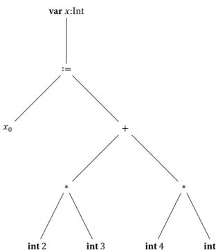
Following Krebbers et al. [37], we can adapt and extend the zipper to model program execution: The focus shall be on (sub)expressions in our model language and the context will consist of the expression turned inside-out representing a path from the focused subexpression to the whole expression, i.e. the steps executed in the current scope to reach the focused subexpression. We will illustrate this with an example based on theScala Coreprogram given in Listing 26:

var x: Int;

x := 2*3+4*5

Listing 26:A SimpleScala CoreProgram

int2 int3 int4 int5

∗ ∗

𝑥0 +

∶= var𝑥:Int

Figure 15:The Parse Tree of Listing 26

When we focus the rightmost multiplication, the context can be once again visualized – as shown in Fig. 16.

int2 int3

∗

𝑥0 +

∶= var𝑥:Int

Figure 16:The Parse Tree of Listing 26

int6

ref𝑎𝑥 +

∶= var𝑥:Int

Figure 17:The Visualized Context of4*5in Listing 26 with evaluated expressions

Instead of using figures of trees, orScalaprograms, we shall express the context of a focused expression in lists of what we shall call singular expression contexts. For the given example we shall define a number of singular expression contexts – as shown in 18:

⟨𝑏𝑜𝑝⟩ ∶∶=; ∣ + ∣∶=∣ ∗ ∣ …

𝐾𝒮∶∶=⟨𝑏𝑜𝑝⟩ 𝑒2∣ 𝑣1⟨𝑏𝑜𝑝⟩∣ var𝑎

Figure 18:Singular program contexts

The meaning of these singular contexts is as follows:

• The two binary expression contexts,⟨𝑏𝑜𝑝⟩ 𝑒2and𝑣1⟨𝑏𝑜𝑝⟩, mark the currently focused statement as

either the left or right subexpression of a binary expression. if the binary expression context is of the second subexpression, the first subexpression has been evaluated to a value.

• The variable block contextvar𝑎marks the current expression as the subexpression of a variable block, where

the address of the variable is𝑎.

We will add more singular expression contexts to the definition as they are required, e.g. when dealing with function calls.

Using these singular expression contexts, we can now succinctly express the context of4*5in the simple program – as shown in Fig. 19.

𝐤 =int6 +

∶∶ref𝑎𝑥∶=

∶∶ var𝑎_𝑥 ∶∶ []

Figure 19:The Context of4*5in Listing 26

the form6 +. The context of the addition is right hand side of the assignment where the left hand side isref𝑎𝑥, i.e.

ref𝑎𝑥∶=. Finally the context of the addition is the variable declarationblock𝑎𝑥.

As before, we can traverse upwards and downwards along the zipper, in this case to subexpressions and superexpres-sions respectively. For instance, if we move downwards from4*5, the focus shall change to4, with the following context:

𝐤 =∗int5

∶∶int6 +

∶∶ref𝑎𝑥∶=

∶∶ var𝑎_𝑥 ∶∶ []

Figure 20:The Context of4in Listing 26

In the same fashion, if we move upwards from4*5, the focus changes to2*3+4*5, with the following context:

𝐤 =ref𝑎𝑥∶=

∶∶ var𝑎_𝑥 ∶∶ []

Figure 21:The Context of2*3+4*5in Listing 26

The practical effect of defining the data structure in this fashion, is that each focused statement comes with the execution history relevant to its scope, in the form of the context. It is this history which allows us to add non-local effects to the semantics. In the next section we will demonstrate the program contexts in action, as we shall describe the basic structure of program context semantics.

4.3

Scala Core

with only Basic Expressions

For this first foray into program context semantics for aScala Core, we will have a look at the simple expression language which will form the base of our model language. First we will define a syntax for this basic language, then we will provide and explain the runtime structures necessary for the semantics and provide a number of reduction rules and finally we will give a a sample reduction of a small program.

4.3.1 Syntax

The syntax of the basic expression language is defined as follows:

Type ∶∶=RefType ∣Int∣Unit

Value ∶∶=refAddress ∣intInteger ∣unit

Integer = ℕ

Address = ℕ

There are only 3 types:Pointer, which is the type of addresses in memory, parametrized with the type of the element it points to,Int, the type of integer values and theUnittype. Corresponding to these types we have pointer values, integer values and the unit instance. The unit instance can not be directly used, but is used as the return type of expressions such as assignment.

In the semantics, we will generally refer to types as𝑡𝑖, values as𝑣𝑖and addresses as𝑎𝑖, with𝑖 ∈ ℕ, dropping the

subscript in the singular case.

We have the following expressions, which we will refer to using𝑒𝑖:

⟨𝑏𝑜𝑝⟩ ∶∶=; ∣∶=

Expression ∶∶= Expression ⟨𝑏𝑜𝑝⟩ Expression ∣loadExpression ∣varType; Expression ∣ 𝑥𝑖

∣ Value

Figure 23:Expressions in the Basic Expression Language

• Assignment𝑒1∶= 𝑒2, which stores a value to a location on the heap. It will evaluate tounit.

• Sequential𝑒1; 𝑒2, which evaluates two expressions sequentially. It will evaluate to the value of the second

expression.

• Loadload𝑒, which loads a value from a given address in the heap.

• VarBlockvar𝑡; 𝑒, which declares a variable of type𝑡. The variable has no name, as we refer to variables by their position on the stack instead of by name.

• Ident𝑥𝑖, which provides the value at the𝑖𝑡ℎposition of the stack.

4.3.2 Semantics: Runtime Structure

For our model language we shall give a small-step operational semantics which makes extensive use of the previously introduced program contexts.

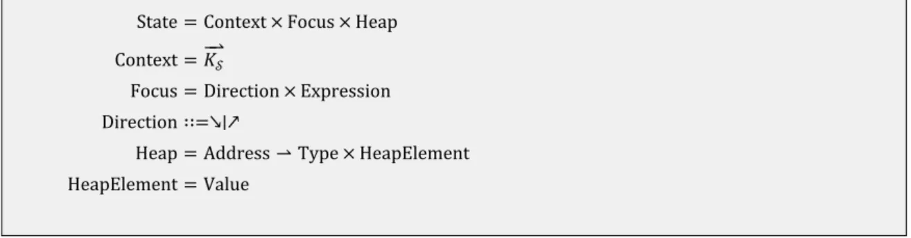
For this we need to define the runtime state of our semantics:

State = Context × Focus × Heap

Context =−𝐾⇀𝒮

Focus = Direction × Expression

Direction ∶∶=↘∣↗

Heap = Address ⇀ Type × HeapElement

HeapElement = Value

Figure 24:Runtime Structure

States consist of a context, a focus and a heap. We will refer to states as𝑆𝑖and use the syntactic shorthand𝑆𝑖 =

S(𝑘, 𝜙, ℎ).

With only primitive types, a heap is a finite partial function from addresses to pairs of a type and a value; we shall refer to them usingℎ𝑖. We shall use the shorthandℎ[𝑎 ↦ 𝑣]to store values in the heap and useℎ[𝑎 ↦ ⊥]to allocate

Contexts are lists of singular expression contexts, as described in Section 4.2. We generally refer to them using𝑘𝑖. We

shall define the singular expressions for the simple language in Fig. 25.

Foci consist of the currently focused expression, i.e. the actual focus of the zipper, and a direction. The direction indicates where the focus will be moved in the next state; up↗, or down↘the parse tree of the expression. We will refer to foci using𝜙𝑖.

In this simple variant of our model language we have the following singular expression contexts:

⟨𝑏𝑜𝑝⟩ ∶∶=; ∣∶=

𝐾𝒮∶∶=⟨𝑏𝑜𝑝⟩ 𝑣2∣ 𝑒1⟨𝑏𝑜𝑝⟩∣ var𝑎∣ load

Figure 25:Basic Singular Expression Contexts

Most of the basic singular expression contexts are already familiar from Section 4.2, but we have addedload, which is used to provide the context for the subexpression𝑒inload𝑒expressions.

The stack𝜌, which is implicitly contained in𝑘, consists not of values, but of pointers to values on the heap, which will simplify capturing local variables by closures, as all captured variables will consist of references to heap-allocated variables. To prevent closures from referring to non-existing variables, variables are not explicitly deallocated when they go out of scope; a garbage collector is assumed to prevent heap pollution. We will refer to the stack using DeBruijn-indices [14] instead of names, meaning that instead of variable names we shall use𝑥𝑖which will refer to the 𝑖𝑡ℎvariable-adress on the stack; this means we do not need special handling of overlapping variable names in different scopes.

The implicit availability of𝜌in𝑘is made possible by the fact that there are singular expression contexts marking every variable allocation. To illustrate this, we look at the example in listing Listing 27:

f(x: Int) : Unit {

var y: Int;

y := 5

}

f(6)

Listing 27:Stack Example

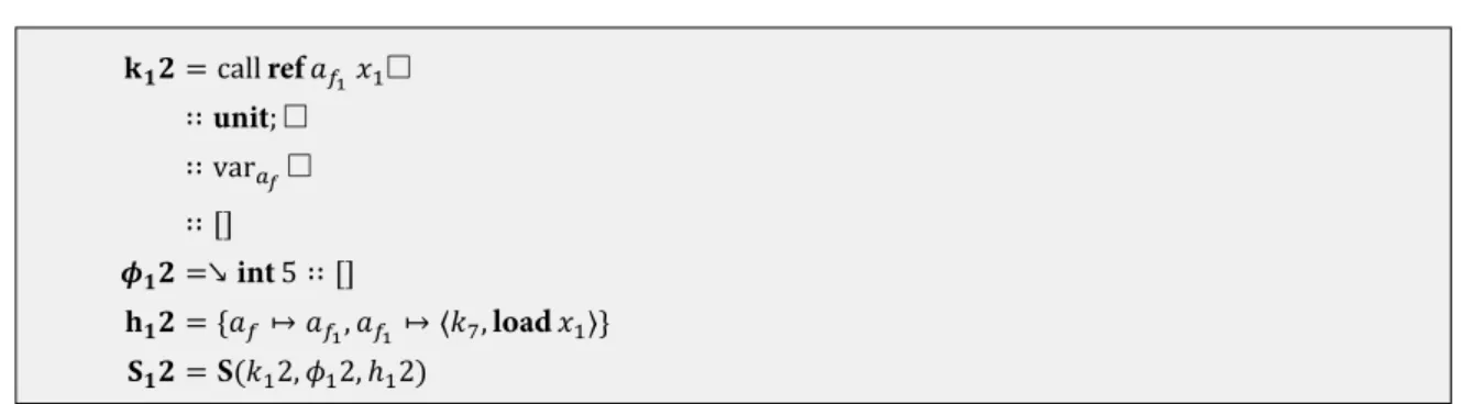
The example program which we use to illustrate the stack implicitly contained in the context, shows a simple function definition and its call. This is one extension past the simple expression language, but it allows for a more effective illustration. The context of interest will be the one wherey:=5is the focussed statement, in the execution of the function body; we provide this context in Listing 28.

𝐤 = var𝑎𝑦

∶∶ funCall 𝑐𝑐 ⟨6⟩

∶∶ var𝑎𝑓

∶∶ []

Listing 28:The Context ofy:=5in Listing 27

which we shall examine in detail in Section 4.4; for now it is important to know that this context contains adresses of the evaluated parameters to the function in the form of−⇀𝑎.

The stack at the time of the assignment consists of the local variable𝑦, the parameters to the function and the variable 𝑓, which is part of the lexical closure of the function. These values are contained in the program context, in the singular var𝑎_𝑦,funCall 𝑐𝑐 ⟨6⟩andvar𝑎_𝑓contexts respectively. In the general case, the concatenation of the addresses, in singular

variable contexts, and the parameters, in singular function call contexts, will provide the stack, in this fashion. We therefore define a𝑔𝑒𝑡𝑆𝑡𝑎𝑐𝑘function in Listing 29, which provides us the stack. We treat this function as an implicit conversion where needed and extend this function as more singular expression contexts are defined.

getStack(⟨𝑏𝑜𝑝⟩ 𝑒2∶∶ 𝑘) ∶= getStack 𝑘

getStack(𝑣1⟨𝑏𝑜𝑝⟩∶∶ 𝑘) ∶= getStack 𝑘

getStack(var𝑎 ∶∶ 𝑘) ∶= 𝑎 ∶∶ getStack 𝑘

getStack(funCall−⇀𝑣 ∶∶ 𝑘) ∶=−⇀𝑣 ⧺ getStack 𝑘

Listing 29:A Function to Derive the Stack from the Context.

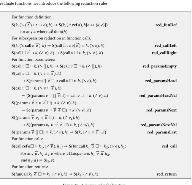
4.3.3 Semantics: Reduction Rules

With the runtime structure defined in the previous section, we can now define the operational semantics for the simple expression language with the following reduction rules:

For the skip expression:

S(𝑘, (↘skip), ℎ) ⇾S(𝑘, (↗unit), ℎ) red_skip

For subexpression reduction in binary expressions:

S(𝑘, (↘ 𝑒1⟨𝑏𝑜𝑝⟩ 𝑒2), ℎ) ⇾S(⟨𝑏𝑜𝑝⟩ 𝑒2∶∶ 𝑘, (↘ 𝑒1), ℎ) red_binSubLeft

S(⟨𝑏𝑜𝑝⟩ 𝑒2∶∶ 𝑘, (↗ 𝑣1), ℎ) ⇾S(𝑣1⟨𝑏𝑜𝑝⟩∶∶ 𝑘, (↘ 𝑒2), ℎ) red_binSubRight

S(𝑘, (↘ 𝑒1⟨𝑏𝑜𝑝⟩ 𝑣2), ℎ) ⇾S(⟨𝑏𝑜𝑝⟩ 𝑣2∶∶ 𝑘, (↘ 𝑒1), ℎ) red_binSubLeftVal

S(𝑘, (↘ 𝑣1⟨𝑏𝑜𝑝⟩ 𝑒2), ℎ) ⇾S(𝑣1⟨𝑏𝑜𝑝⟩∶∶ 𝑘, (↘ 𝑒2), ℎ) red_binSubRightVal

For binary expressions:

S(; 𝑣2∶∶ 𝑘, (↗ 𝑣1), ℎ) ⇾S(𝑘, (↗ 𝑣2), ℎ) red_seqLeft

S(𝑣1;∶∶ 𝑘, (↗ 𝑣2), ℎ) ⇾S(𝑘, (↗ 𝑣2), ℎ) red_seqRight

S(∶= 𝑣 ∶∶ 𝑘, (↗ref𝑎), ℎ) ⇾S(𝑘, (↗unit), ℎ[𝑎 ↦ 𝑣]) red_assignLeft

S(ref𝑎 ∶=∶∶ 𝑘, (↗ 𝑣), ℎ) ⇾S(𝑘, (↗unit), ℎ[𝑎 ↦ 𝑣]) red_assignRight

For variable declaration blocks:

S(𝑘, (↘ (var𝑡; 𝑒)), ℎ) ⇾S(var𝑎 ∶∶ 𝑘, (↘ 𝑒), ℎ[𝑎 ↦ ⊥]) red_varBlock

for any𝑎where𝑎 ̸∈ dom(ℎ)

S(var𝑎 ∶∶ 𝑘, (↗ 𝑣), ℎ) ⇾S(𝑘, (↗ 𝑣), ℎ) red_varBlockUp

S(𝑘, (↘var𝑡; 𝑣), ℎ) ⇾S(𝑘, (↗ 𝑣), ℎ) red_varBlockVal

For variable lookup:

S(𝑘, (↘load𝑒), ℎ) ⇾S(load∶∶ 𝑘, (↘ 𝑒), ℎ) red_loadSub

S(load∶∶ 𝑘, (↗ref𝑎), ℎ) ⇾S(𝑘, (↗ 𝑣), ℎ) red_load

for any𝑣wheresnd ℎ(𝑎) = 𝑣

The basic reduction rules have the following meaning:

• red_binSubLeftevaluates a binary expression one step by marking the first subexpression for evaluation using ↘and prepending a singular binary expression context containing the second subexpression and with a hole for the first.

• red_binSubRightmarks the second subexpression of a binary expression for execution, when it encounters the resulting value of the first subexpression combined with a singular binary expression context. It swaps the encountered singular binary expression context with a hole for the first subexpression, with one for the second subexpression.

• red_binSubLeftValmarks the second subexpression of a binary expression for execution, in case the first one is already a value, skipping the evaluation of the first subexpression.

• red_binSubRightValfinishes up the subexpression reduction of a binary expression, when it encounters a value for the second subexpression and the resulting value of the first subexpression in a singular binary expression context, by removing the singular binary expression context and marking the binary expression for execution, now with values instead of expressions.

• red_seqLeftandred_seqRightevaluate a sequential expression, by discarding the value resulting from the first subexpression and propagating the value of the second subexpression.

• red_assignLeftandred_assignRightassign value𝑣to address𝑎in the heap. The value of an assignment expression is alwaysunit.

• red_varBlockdeclares a local variable by prepending a singular var context, with𝑎the address of the variable, which implicitely pushes𝑎on the stack. The variable is uninitialized.

• red_varBlockUpremoves a singular var context, consequently removing the variable from the stack. It does not deallocate the variable from the heap, as it could have been captured by a function closure. The value of a block is the value of its expression.

• red_varBlockValremoves a singular var context, consequently removing the variable from the stack. It does not deallocate the variable from the heap, as it could have been captured by a function closure. The value of a block is the value of its expression.

• red_loadSubevaluates the subexpression in a load expression.

• red_loadevaluates a load expression from address𝑎to the value stored in the heap at that address.

4.3.4 Reduction of a Simple Program

Since we have defined the semantics formally, let us run through the reduction of a simple program to see them in action:

var x : Int;

x := 5;

x := 3

Listing 31:Simple Program for Reduction Example

𝐤𝟏= []

𝝓𝟏=↘varInt; 𝑥0∶=int5; 𝑥0∶=int3

𝐡𝟏= {}

𝐒𝟏=S(𝑘1, 𝜙1, ℎ1)

Figure 26:The Initial State in the Reduction of Listing 31

The initial state of the reduction of Listing 31 is given by Fig. 26: The context𝑘1consists of an empty list, as we are at

the top expression, and the heapℎ1starts empty as well. The focused expression𝜙1is a variable block, which will

declare the local variable𝑥for the expression𝑥0∶=int5; 𝑥0∶=int3, which means thered_varBlockrule applies –

resulting in the state of Fig. 27.

𝐤𝟐= var𝑎_𝑥 ∶∶ []

𝝓𝟐=↘ 𝑥0∶=int5; 𝑥0∶=int3

𝐡𝟐= {𝑎𝑥↦ ⊥}

𝐒𝟐=S(𝑘2, 𝜙2, ℎ2)

Figure 27:The Second State in the Reduction of Listing 31

After applyingred_varBlock, we have reached the second state of the reduction: A singular var context with the address of𝑥has been appended to the context, making the address of𝑥the zeroeth of the stack. The variable𝑥has been defined and now points to an empty location in the heap. The focus is now on the sequence subexpression in the scope of the block, which has been marked for execution using↘. This means thered_binSubLeftrule applies – resulting in the state of Fig. 28.

𝐤𝟑=; 𝑥0∶=int3

∶∶ var𝑎𝑥 ∶∶ []

𝝓𝟑=↘ 𝑥0∶=int5

𝐡𝟑= {𝑎𝑥↦ ⊥}

𝐒𝟑=S(𝑘3, 𝜙3, ℎ3)

Figure 28:The Third State in the Reduction of Listing 31

In the third state,red_binExphas been applied, which resulted in a singular sequence context being appended to the context, which signifies that we are executing the first subexpression of the sequence. The focused statement consists of this first subexpression, which is the assignment𝑥0∶=int5, marked for execution using↘. While the right hand

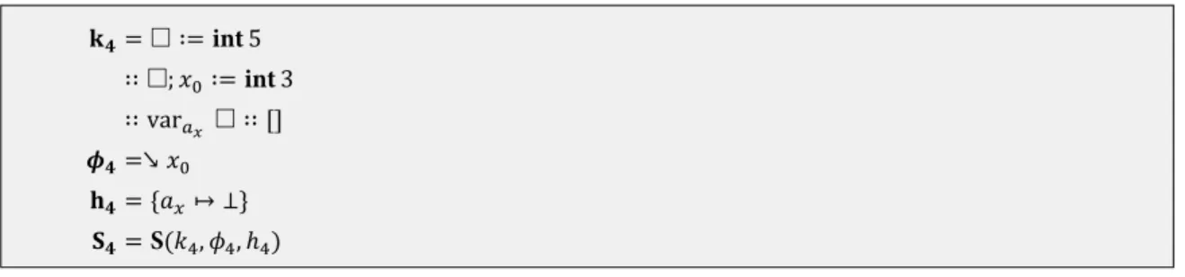
𝐤𝟒=∶=int5

∶∶; 𝑥0∶=int3

∶∶ var𝑎_𝑥 ∶∶ [] 𝝓𝟒=↘ 𝑥0

𝐡𝟒= {𝑎𝑥↦ ⊥}

𝐒𝟒=S(𝑘4, 𝜙4, ℎ4)

Figure 29:The Fourth State in the Reduction of Listing 31

In the fourth state,red_binSubLeftValhas been applied and the variable corresponding to the first element of the stack evaluates to the address of the variable𝑥. Since the first subexpression has been reduced and the second is already a value, we can now applyred_assignLeft– resulting in the state of Fig. 30.

𝐤𝟓=; 𝑥0∶=int3

∶∶ var𝑎𝑥 ∶∶ []

𝝓𝟓=↗unit

𝐡𝟓= {𝑎𝑥↦ 5}

𝐒𝟓=S(𝑘5, 𝜙5, ℎ5)

Figure 30:The Fifth State in the Reduction of Listing 31

In the fifth state, the application ofred_assignLefthas resulted in the heap changing, to reflect the assignment of the integer value5to𝑥, and the direction of the focused statement changing to↗. This direction combined with the singular sequential context, with theon the left side, at the head of the context, means thered_binSubRightrule now applies – resulting in the state of Fig. 31.

𝐤𝟔=unit;

∶∶ var𝑎_𝑥 ∶∶ [] 𝝓𝟔=↘ 𝑥0∶=int3

𝐡𝟔= {𝑎𝑥↦ 5}

𝐒𝟔=S(𝑘6, 𝜙6, ℎ6)

Figure 31:The Sixth State in the Reduction of Listing 31