BACHELOR THESIS
MODEL FITTING FOR
ALTERNATIVE STATISTICAL
MODELS FOR BINARY
SURVEY DATA
Konrad Klotzke
DEPARTMENT OF RESEARCH
METHODOLOGY, MEASUREMENT AND DATA ANALYSIS
Enschede, June 2015
EXAMINATION COMMITTEE
1
Abstract
Strong empirical evidence suggests that respondents are more likely to respond truthfully to
a sensitive question if they feel that the anonymity and confidentiality of their response is
granted. The Randomized Response Technique provides an approach to increase the
response accuracy on sensitive questions while allowing a valid estimation of the
prevalence of illegal or socially undesirable behavior and attitudes in the population. It was
assumed that existing goodness-of-fit tests are suited for Randomized Response designs
with binary data if the link function is adjusted. The assumption was evaluated in a
simulation study for categorical and continuous data. Across a total amount of 210000
randomly generated samples, no significant difference in type-1 errors was found between
randomized data and non-randomized data. The statistical power declined as the degree of
randomization of the data was increased. No difference between categorical and continuous
data was found. The obtained results strongly indicate that existing goodness-of-fit tests can
2
Table of Contents
Abstract ... 1
1. Introduction ... 5
1.1 Surveys ... 5
1.2 Error and bias... 5
1.3 Sensitive questions and response accuracy ... 6
1.4 Increasing the response accuracy on sensitive questions... 7
2. Representing Randomized Response Models in Generalized Linear Models ... 8
2.1 Predicting responses using linear regression ... 8
2.2 Generalized Linear Models ... 9
2.3 Generalized Linear Models with a linear link function ...10
2.4 Generalized Linear Models with a logit link function ...10
2.5 Randomized response in Logistic regression models ...11
3. Randomized Response Models ...13
3.1 Warner ...13
3.2 Forced-Response ...14
3.3 Two Bernoulli distributions ...14
4. Problem description...16
4.1 Hypothesis testing and model choice ...16
4.2 Measures of goodness-of-fit ...17
4.3 Goodness-of-fit tests for RR models for binary data ...19
4.4 Evaluating the goodness-of-fit of one model against a single alternative ...20
4.5 Research question ...21
5. Method ...22
5.1 Procedure and technical implementation in R ...22
5.2 Randomized Response designs ...24
5.3 Components of the simulation...24
3
5.3.2 Logistic regression with a continuous predictor and controlled cluster size ...25
6. Data analysis ...27
6.1 Logistic regression with categorical predictors ...27
6.2 Logistic regression with a continuous predictor and controlled cluster size ...28
7. Discussion ...36
7.1 Do the type-1 and type-2 error rates change in an RR design with categorical data, and in what way? ...36
7.2 Do the type-1 and type-2 error rates change in an RR design with continuous data, and in what way? ...36
7.3 Conclusion ...36
4
List of Figures
Figure A: Simulation modules design diagram ...23
Figure B: Type-1 errors for categorical predictors and different RR designs ...30
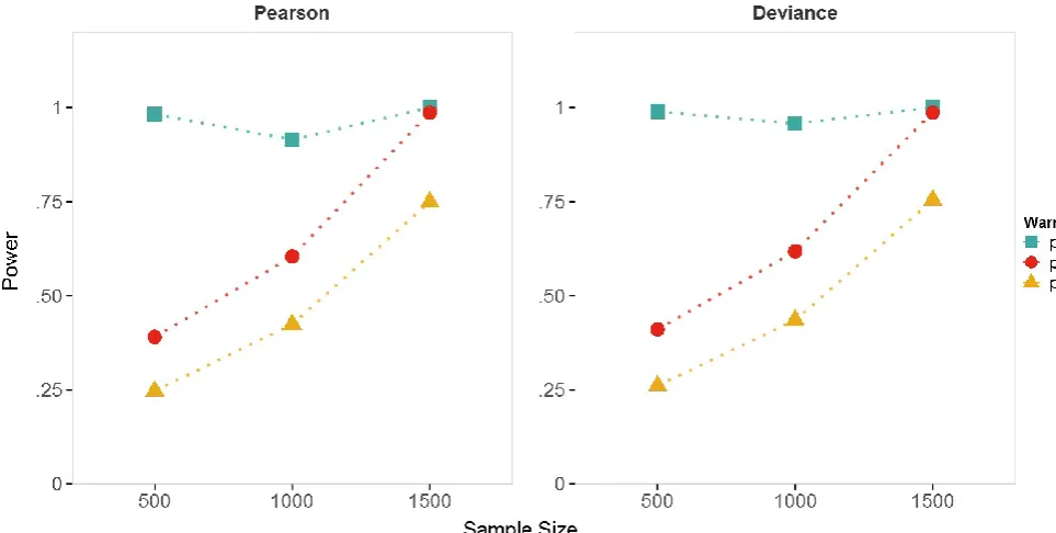
Figure C: Statistical power for categorical predictors and different RR designs ...31
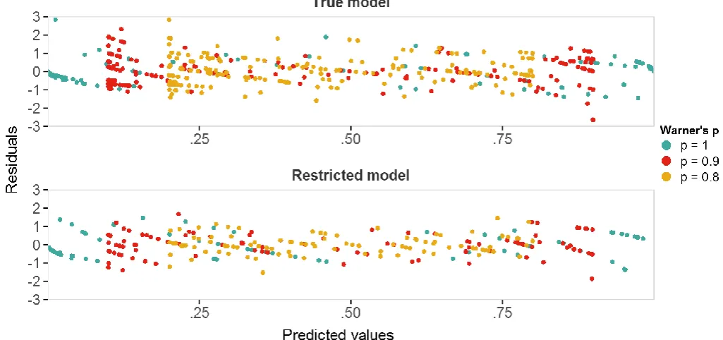
Figure D: Residuals for different RR designs against fitted values ...32
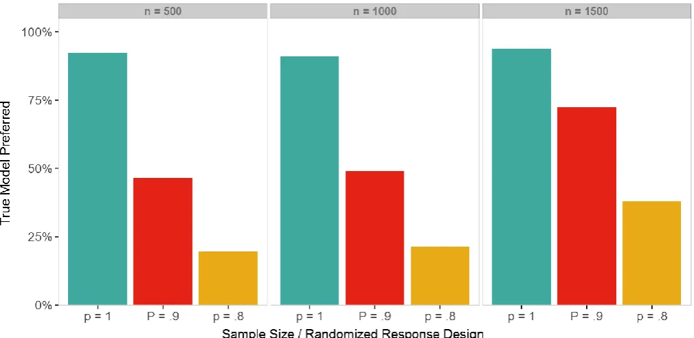
Figure E: Goodness-of-fit of the true model against a single incorrect alternative ...33
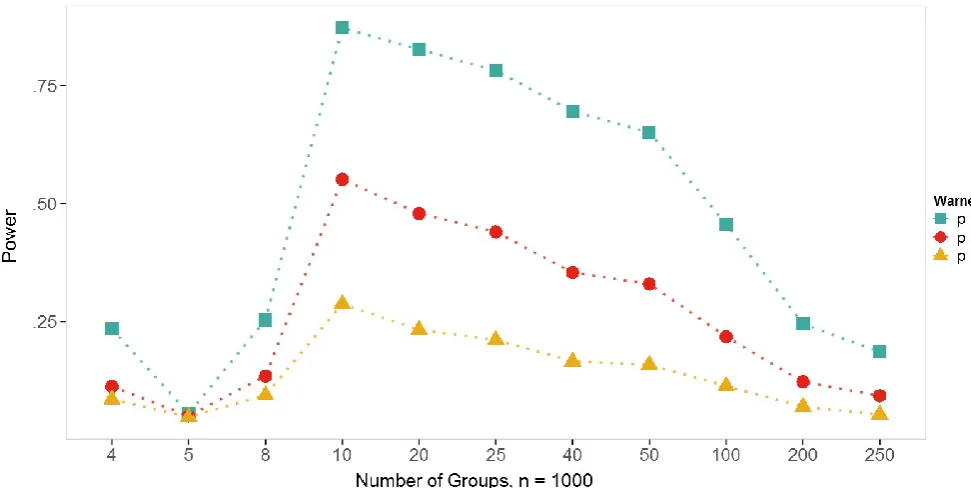
Figure F: Statistical power for different RR designs across different cluster sizes ...34
Figure G: Type-1 errors for different RR designs across different cluster sizes ...35
List of Tables Table A: Data collection designs with parameters c and d...24
Table B: Type-1 error rate for RR data collection designs compared to a non-RR design ...29
5
1. Introduction
1.1 Surveys
During the past decades surveys have served a major role in collecting empirical data for the
purpose of social observational studies. In general, a survey consists out of a set of questions
or statements that, when answered, judged or commented by a representative sample of
respondents, give insight into the prevalence of one or more predefined constructs within
the population the study is aimed at. For example, a study aiming to explore the construct of
intrinsic motivation among students of Dutch universities could utilize a survey that
contains a set of questions that cover all aspects of the construct intrinsic motivation. As it is
often impracticable to collect data from the whole population, in this case the data of all
students of Dutch universities, a representative sample is being studied. In other words, a
sample of the population takes the survey which yields data that aims to be representative
for the whole population.
1.2 Error and bias
Even though there exists a great variety of methods when it comes to selecting a sample
(Hibberts et al., 2012), it is virtually impossible to draw a sample that perfectly represents
the population that it is drawn from. The difference between the data obtained through
applying a sampling method and the true values, as present in the population, is called the
sampling error. If the difference randomly varies with each sample taken, this error is also
referred to as random error. Random error must be distinguished from systematic error, or
bias, which describes a systematic difference in one direction.
According to the Total Survey Error approach, error within survey studies can be
discriminated into three categories (Weisberg, 2005). The first category leads to what is also
called the sampling error, while the second and third category is often unified as the
nonsampling error (Krumpal, 2011). First of all, error can occur at the selection of
respondents, for example in the form of nonresponse bias or sampling bias. Nonresponse
bias means that members of a sample do not become respondents due to a common
characteristic, e.g. if the survey is offered solely in Dutch, international students that do not
speak Dutch systematically will not participate. If the respondents are not selected
randomly but for example by asking for volunteers through a notice at the bulletin board
6 high intrinsic motivation are more likely to voluntarily take part in a study that does not
lead to an extrinsic reward such as extra study points or money.
Second, error can be introduced when processing and analyzing the data as well as when
reporting the results. Potential causes of postsurvey error are mistakes that might occur
when entering the data from a pen-and-paper survey into a computer and applying the
wrong statistical method which leads to a false estimation of the prevalence of the studied
construct in the population.
And finally, a variety of factors influence the accuracy of the responses. In surveys, the
accuracy of a response can be defined as the extent to which the respondent answers in
accordance with the intentions of the researcher (Weisberg, 2005). Weisberg (2005)
furthermore separates response accuracy as measurement error and nonresponse error.
Measurement error can be caused either by the interviewer or the respondent.
Interviewer-related measurement error occurs if the observed responses differ because of the
interviewer. Respondent-related measurement error reflects the discrepancy between the
expected and the observed value. This can range from simple factual checks, e.g. “Did you
ever drink and drive?” in which the researcher expects an answer that matches reality, to
questions about attitude, e.g. “Do you think driving under the influence of alcohol should be
punished more severely?” on which the respondent should provide an answer that is in
accordance with the theoretical model. In other words, if the theoretical model expects that
a respondent who scores high or low on a certain construct provides certain answers, then
any discrepancy between the expected and the observed value increases the measurement
error, lowers the response accuracy, and hence contributes to the total error of the survey.
In some cases a respondent is unable or not willing to answer a question, which causes
nonresponse error at the item level. Nonresponse error at the item level often leads to
biased results as the likelihood to respond to a particular question can be governed by
certain characteristics of the respondent, such as his attitudes and his current or past
behavior.
1.3 Sensitive questions and response accuracy
Questions about topics that are perceived as private or taboo by the respondent, such as
sexual behavior, as well as questions about attitudes and activities that are in contradiction
7 Tourangeau, Rips, and Rasinski (2000) identified three aspects of these so-called sensitive
questions which affect the response accuracy.
The first aspect of sensitivity is the intrusiveness of a question. A question is intrusive to a
respondent if he feels like it invades his privacy by touching a topic that he considers too
private or taboo. Examples of topics that are commonly regarded as intrusive refer to the
income (Moore et al., 2000) and the sexual behavior of the respondent (Fenton et al., 2001).
Another aspect that affects the sensitivity of a question is the perceived risk of disclosure
and possible negative consequences of providing a truthful answer. A student might for
example hesitate to truthfully respond to a question about committing fraud during exams
as he fears that his response might be disclosed, leading to a severe punishment by his
university. Lastly, the sensitivity of a question is influenced by social desirability. Randall
and Fernandes (1991) describe social desirability in terms of two dimensions: a personal
dimension and an item-related dimension. The personal dimension refers to the
respondent’s need of approval as a stable trait. According to the item-related dimension,
respondents judge possible answers of questions based on how far these answers conform
with social norms. From that follows that the degree of perceived sensitivity of a question
depends on the respondent’s need of approval and how the respondent judges the social
desirability of the answer that he is supposed to present under the condition of answering
truthfully.
To sum up, the perceived sensitivity of a question depends as well on the question as on the
answer. A question can touch topics that are too private for the respondent to talk about,
regardless of possible answers. On the other hand, whether or not social desirability
influences the perceived sensitivity of a question depends on if the respondent’s truthful
answer is in conformance with social norms. To illustrate this with an example, the question
“How many sexual partners have you had in the past year?” is likely to be perceived as
touching on a private topic and thus as sensitive while the question “Have you ever
committed rape?” is perceived as sensitive only by those respondents that would answer
with a “yes”. Finally, the perceived risk of disclosure contributes to the perceived sensitivity
of a question.
1.4 Increasing the response accuracy on sensitive questions
First described by Warner (1965), the random response technique (RRT) offers a solution to
8 traditional direct questioning (DQ) methods, the RRT does not require the respondent to
reveal his answer to the researcher. Instead, using a randomizing device, e.g. rolling a dice,
the respondent decides whether he presents his truthful answer or a prescribed response.
The researcher has no insight into the randomizing device and thus the anonymity and
confidentiality of the respondent is granted. In other words, it is not possible for the
researcher to identify the information that belongs to a certain respondent and it is also not
possible to identify the respondent by the information he provided. This successfully
addresses the sensitivity of questions, the sensitivity of answers and the fear of disclosure.
While the researcher cannot draw conclusions about a single respondent, there is strong
evidence that applying the RRT can lead to a valid estimation of the prevalence of illegal or
socially undesirable behavior and attitudes in the population (Lensvelt-Mulders et al., 2005;
Silva & Vieira, 2009; Simon et al., 2006).
2. Representing Randomized Response Models in Generalized Linear Models
2.1 Predicting responses using linear regression
Imagine a researcher theorizing that the performance on a particular task of university
students depends on the students’ intrinsic motivation towards their study and their
intelligence. Here, we have three variables: the response variable , which is the measured
task performance in a controlled laboratory environment of the i-th student, and a set of two
explanatory variables and , representing the intrinsic motivation of the i-th student,
respectively his intelligence. By applying linear regression to the data gained through a
drawing a sample, the researcher can create a function ( ), with being a vector of
explanatory variables to predict the response variable . More concrete, applying linear
regression leads the a linear function ( ), that consists out of the explanatory variables
... , a constant and the regression coefficients ... that determine the weight of the
j-th explanatory variable xij in predicting . From that follows the equation
= ( ) = + ∙ + ⋯ + ∙
with being the predicted response for the i-th respondent. The constant and the
regression coefficients ... are calculated in a way that the sum of the squared
differences between the observed response variable and predicted response variable is
minimized. Hence, unless all observed responses lay on a straight line, each observed
response can differ from its predicted response. The difference between and is named
9
̂ = −
The fitting error is an estimation based on sample data of the of the unknown statistical
error in the population, which captures the influence of any variables other than the
explanatory variables on . The equation for the observed response variable according to
the linear model is thus:
= ( ) +
2.2 Generalized Linear Models
Williams et al. (2013) distinguish three categories of assumptions underlying the
application of the linear regression to sample data in order to yield valid results. First of all a
linear relationship between the response variable and the regression coefficients ...
is assumed. Second, the errors are required to be independent and normally distributed
with a mean of zero and a constant, finite variance across all levels of the explanatory
variables. Finally, it is assumed that the explanatory variables are measured without error.
First described in by Nelder and Wedderburn (1972), the Generalized Linear Model (GLM)
not only allows non-linear relationships between the response variable and the explanatory
variables, but also removes the requirement of having a constant, normally distributed error
for all levels of the explanatory variables (Fox, 2008). The GLM consists out of three parts
(Agresti, 2015): the random component, the linear predictor and the link function. The
random component represents the response variable and its probability distribution. The
observed responses are assumed to be independent. The second component is the linear
predictor which, similar to a linear model equation, may contain explanatory variables,
regression coefficients and constants:
= + ∙ + ⋯ + ∙
Finally, the link function defines how the linear predictor is connected to the mean of the
predicted response variable thus It can be specified as:
( ) = = + ∙ + ⋯ + ∙
Instead of assuming that the variance of the errors ɛ is constant across all levels of the
10 variance function can either depend on the mean, on the predicted value of the response
variable or be a constant.
2.3 Generalized Linear Models with a linear link function
A linear model is the most simple implementation of a GLM as the link function equals the
mean predicted response variable :
( ) = = + ∙ + ⋯ + ∙
As noted above, this can also be written as
= + ∙ + ⋯ + ∙ +
with the error having an estimated mean of ̂ = 0 and a variance of ( ) = ( ) =
σ .
2.4 Generalized Linear Models with a logit link function
While linear models can be utilized to predict a continuous, normally distributed response
variable, research in social science often calls for the prediction of a dichotomous outcome
(Peng et al., 2002). Predicting a dichotomous outcome follows from asking questions such as
whether a student will pass a course or whether a teenager will engage in risky behavior. In
other words, a dichotomous outcome is either a success or a failure and the researcher is
interested in predicting the probability of the observed outcome being a success.
Furthermore predicting dichotomous outcomes can help the researcher or stakeholders to
take decisions, such as classifying a child as learning disabled.
Logistic regression offers a solution to predict dichotomous outcomes by utilizing the
natural exponential function:
= ( = 1| ) =
∙ ⋯ ∙
1 + ∙ ⋯ ∙
Here, ( = 1| ) is the probability that the outcome is a success for a given vector of ,
... are explanatory variables, is a constant and ... are regression coefficients. The
response variable, hence the probability, follows a Bernoulli distribution with a variance of
∙ (1 − ), thus ~ ( ∙ (1 − )). Translated into a GLM the logistic regression
11
= + ∙ + ⋯ + ∙
( ) = ( ) = = log 1 −
( ) = = 1 + ( ) = ∙ (1 − )
The link function ( ) can be any function that maps continuous values from [−∞, ∞] to
[0,1]. However, as a result of its intuitive interpretation as the log of the odds of the
successes, thus on average for every failure there will be /(1 − ) successes, the logit
function is commonly used for this purpose. By applying regression to the linear predictor,
the predicted logit can be computed for each level of the explanatory variables.
Furthermore, the predicted logit can be converted to a predicted probability value by
utilizing the inverse link function ( ). Finally, the variance is calculated based on the
predicted probability using the function ( ).
2.5 Randomized response in Logistic regression models
Under the presumption that the respondent follows the instructions provided by the
researcher, van den Hout, van der Heijden and Gilchrist (2007) demonstrated that the
Randomized Response (RR) models described by Warner (1965), Boruch (1972) and Kuk
(1990) can be represented models by a single equation:
( ∗= 1) = + ∙ ( = 1)
( ∗= 1) is the probability that the first answer, e.g. “yes”, is being observed from the i-th
respondent, ( = 1) is the probability that the i-th respondent gives the first answer and
the parameters c and d model the noise that is introduced if utilizing the randomized
response technique (RRT) during data collection. Veen (2014) and Fox, Klotzke and Veen
(2015) further extended the set of RR models represented by the single equation.
Rearranging the equation to solve for ( = 1) enables the specification of the according
link function in the GLM:
∗ = ( ∗= 1)
= ( = 1) =
12
( = 0) = 1 − = + −
∗
=> ( ∗) = = ( ) = log
1 − = log
∗−
c + d − ∗
The specification of the inverse link function follows the same approach. Given
( ) = ∗
=
∗−
= 1 +
the inverse link function is defined as:
( ) = ∗= + ∙
1 +
Likewise, the equation for the variance function can be set up by simply replacing of the
original equation as defined in the GLM with the according term consisting out of the
parameters ∗, c and d:
( ) = ∙ (1 − )
=
∗−
=> var( ∗) =(
∗− ) ∙ ( + + ∗)
As ∗ follows from Y, it is also Bernoulli distributed based on the predicted value ∗ thus
∗~ ( ∗∙ (1 − ∗)) with ∗= + ∙ ( = 1).
13
3. Randomized Response Models
3.1 Warner
Aiming to protect the privacy of the respondents and by that, increasing the response
accuracy on sensitive questions, in 1965 Warner proposes the historically first random
response (RR) model. In Warner’s model each sensitive question comes along with a
negotiation of the same. For example, the question “Have you consumed drugs in the past
four weeks?” would be presented along with its negotiation “Have you not consumed drugs
in the past four weeks?”. Using a randomizing device, e.g. rolling a dice, the respondent
selects a question to which he provides a truthful answer. The researcher has no insight into
the randomizing device and hence does not know to which of the two questions the
respondent provided an answer. He however is aware of the probability distribution of the
randomizing device and therefore of the probability of the respondent selecting the real
question. For example, if the respondent is instructed to select the real question, as opposed
to the negotiation, if the dice shows a 2, 3, 4, 5 or 6 then the probability for the respondent
to answer the real question is 5/6 and vice versa the probability to choose the negotiated
question is 1/6. This can be expressed with equation given in chapter 2.5 of this paper. First
of all, if the first answer, e.g. “yes”, is observed, it is either possible that it matches the
respondent’s true answer and he is prompted to respond to the real question or that the
respondent’s true answer is actually the opposite but he is prompted to answer the
negotiated question:
( ∗ = 1) = ( ∗= 1| = 1) + ( ∗= 1| = 0)
With p being the probability that the randomizing device leads to instructing the respondent
to answer the real question and π being the true probability of giving the first answer to the
real question, thus (Y = 1) the equation for ( ∗= 1) is as follows:
( ∗= 1) = p ∙ π + (1 − p) ∙ (1 − π)
<=> ( ∗= 1) = π ∙ (2p − 1) + (1 − p)
Finally, the parameters c and d are defined as (1 − p) respectively (2p − 1), which leads to
the following equation:
( ∗= 1) = π ∙ d + c
14 In the aforementioned example of rolling a dice to select either the real question or its
negotiation, c would hence equal 1 − 5/6 = 1/6 and d equals 2 ∗ 5/6 − 1 = 2/3.
3.2 Forced-Response
Contrary to Warner’s model, the forced-response (FR) model, as described by Boruch
(1972), relies on prompting a single, sensitive question to the respondent. Using the
randomizing device, in which the researcher has no insight, the respondent is instructed to
reply with either “yes”, “no” or either “yes” or “no” based on his truthful answer. If a dice is
utilized as randomizing device, the respondent could for example be instructed to reply with
“yes” if the outcome of the dice is a 1, to reply with “no” if the outcome is 6 and to reply
truthfully with either “yes” or “no” if the dice shows a 2, 3, 4 or 5.
With the known probability of an instructed “yes” or “no” reply being respectively , the
probability of a truthful answer is 1 − − . From that follows that the probability for an
observed “yes” is the sum of the probability for the respondent to answer truthfully with
“yes” and the probability of a forced “yes” reply, thus . Defining c as equaling and d as
equaling 1 − − shows that the FR model can be represented by the following equation:
( ∗= 1) = π ∙ 1 − − +
<=> ( ∗= 1) = π ∙ d + c
<=> ( ∗= 1) = c + d ∙ (Y = 1)
3.3 Two Bernoulli distributions
Kuk (1990) offers an RR model in which two separate Bernoulli distributions are used to
add noise to the true answer of the respondent. First, the respondent faces a question that
can be answered with either “yes” or “no”. Next, the respondent is provided with two binary
outcomes that differ in their probability distribution. A concrete example are two packs of
cards. Each pack is shuffled and consists out of blue and yellow cards with the ratio of blue
versus yellow cards differing between the packs. In other words, drawing a card from each
pack leads to two binary outcomes, namely blue or yellow, and the probability for the drawn
card to be blue is higher in one pack. If the respondent’s true answer to the question is “yes”,
then he is asked to show the card drawn from the first pack to the researcher and likewise, if
the respondent’s true answer is “no”, he shows the card drawn from the second pack. The
15 However, as he is aware of the proportion of blue versus yellow cards in each of the two
packs, he possesses insight into the probability distributions of the outcomes.
Let 1 and 2 be the known proportion of blue cards in the first respectively second pack, p1
and p2 are therefore the probabilities to draw a blue card from the first respectively second
pack and being the probability that the respondent would answer with “yes” to the
question. With defining c as equaling p2 and d as equaling (p1 - p2), Kuk’s model can be
represented by the following equation:
( ∗= 1) = ( ∗= 1| = 1) + ( ∗= 1| = 0)
<=> ( ∗= 1) = ∙ π + ∙ (1 − π)
<=> ( ∗= 1) = π ∙ ( − ) +
<=> ( ∗= 1) = π ∙ d + c
16
4. Problem description
4.1 Hypothesis testing and model choice
Goodness-of-fit tests indicate how well a statistical model fits the observed data. In this
simulation the observed data is generated based on the inverse link function which maps
the linear term of explanatory variables and their coefficients thus = + + ⋯ +
to a probability, hence to values between 0 and 1. For the logit link function the
formula looks as follows:
( ) = + ∙ 1 +
Writing the formula in a more general way shows that the mapping can be done with any
link function that maps continuous values from [−∞, ∞] to [0,1]:
( ∗= 1) = c + d ∙ (Y = 1)
Two types of statistical models are used in this paper: First of all, the true model which fully
matches reality and therefore can predict the observed data accurately. In other words, it
contains the complete term of explanatory variables and accurate regression coefficients.
For the purpose of this simulation the true model will therefore use the complete set of
explanatory variables ... and the restricted model contains an incomplete set of
explanatory variables. To illustrate this with a practical example in which the observed data
is generated with two explanatory variables, and : the true model contains the linear
prediction term = 0.2 + 0.4 ∗ − 0.17 ∙ while in the restricted model the effect of
the second predictor is fixed to zero, leading to a linear term based on only the first
predictor , e.g. = −0.1 + 0.6 ∙ .
Two tests for statistical significance can be described. Considering that the true model
matches the model used for simulating the data, a goodness-of-fit test should not indicate a
statistical significant difference between the observed data and predictions from the true
model. In terms of the null hypothesis H0 and an alternative hypothesis Ha, this can be
formulated as follows: H0: there is no significant difference between the observed data and
the predictions of the true model. Ha: there is a significant difference between the observed
data and the predictions of the true model and therefore an alternative model fits the data
17 If this test leads to the incorrect conclusion that H0 must be rejected when the true model is
equal to the model used for generating the data, a so-called type-1 error is made.
The second test concerns the restricted model, which by definition differs from the model
used for generating the data. The corresponding hypotheses are as follows: H0: there is no
significant difference between the observed data and the predictions of the restricted model.
Ha: there is a significant difference between the observed data and the predictions of the
restricted model.
Considering that by definition the restricted model does not fit the data as accurately as the
model used for generating the data, a goodness-of-fit test should lead to the conclusion that
Ha is true and thus that H0 should be rejected. If the conclusion is however that the restricted
model fits the data well enough, then a so-called type-2 error is made. Furthermore, the
statistical power of a test is defined as 1 - the fraction of type-2 errors and hence the
statistical power of a test declines as more type-2 errors occur.
4.2 Measures of goodness-of-fit
For categorical data the Pearson and Deviance goodness-of-fit tests are utilized. While the
exact procedure to compute the goodness-of-fit differs between those two measures, the
general approach is very similar. In short, based on the observed group mean probability ∗
and the predicted group mean probability ∗ the difference between the observed data and
the predictions is computed. As discussed in more detail in the next paragraph, here, each
group consists out of respondents that share the same combinations of explanatory
variables. In simplified terms, the respondents who share the same set of characteristics are
grouped together. For each group, the difference between ∗ and ∗ is furthermore scaled
by the estimated standard deviation within that group. The Pearson statistic is computed
as follows, with being the number of respondents in the i-th group:
= ∙ (
∗− ∗)² ∗∙ (1 − ∗)
For more information on the Pearson and Deviance goodness-of-fit tests see Tutz (2011, pp.
18
Each of the explanatory variables ... represents a certain characteristic of the i-th
respondent. For example the first explanatory variable could contain the age of the
respondent and the second variable could represent his or her gender. If takes the
value 0 for a male and 1 for a female gender, a 30 year old woman would be represented by
= 30 and = 1. Furthermore this woman would have either a positive observed
outcome, i.e. = 1 or a negative outcome, i.e. = 0. Repeating the same procedure for n
– 1 more respondents would result in a total of n individual combinations of , and .
However, for the Pearson and Deviance statistics the degrees of freedom increase along with
the sample size n. As the Pearson test statistic is not guaranteed to be asymptotical
chi-squared distributed for a large degree of freedom, its value cannot be safely evaluated. The
same accounts for the Deviant test statistic (Tutz, 2011, pp. 89-90). The solution is to
group the respondents based on their characteristics. In the former example with two
explanatory variables, the respondents who share the same value of and , would be
placed in the same group, or cluster. For example one cluster contains all 40 year old males,
the next cluster contains all 35 year old females and so on.
Under the assumption that each cluster contains more than one respondent, for each
characteristic, thus combination of explanatory variables, multiple observations are
available. Each cluster with i respondents contains trials for a given combination of
explanatory variables and the outcome of a trial is either a 1 or 0, thus a success respectively
a failure. In other words, the Bernoulli distribution with a single trial for each respondent
has been transformed to a Binominal distribution for each cluster with trails and an
estimated group mean probability , resulting in ~ ( , ). As the number of clusters is
fixed, the test statistic values and can be evaluated with a chi-squared distribution
with N - P degrees of freedom, N being the number of non-empty clusters and P being the
number of estimated parameters.
While the Pearson and Deviance statistics are designed for categorical data, they can also, to
some degree, be applied to continuous variables. In the former example the variable age is
continuous but is treated as categorical due to its discrete character and its fixed number of
possible values, or levels. A continuous variable with a great number of levels would
however strongly increase the number of clusters and as a result the degrees of freedom of
the chi-squared distribution would no longer be fixed. The Hosmer-Lemeshow (H-L) test
approaches this difficulty by offering an alternative way to group the respondents into
19 of grouping respondents based on their shared explanatory variables, the researcher can
choose the number of clusters. The procedure is as follows: first of all, the respondents are
ordered based on their predicted probability of success. As discussed earlier, the predictions
are made for each respondent based on his characteristics, hence his combination of
explanatory variables. Next, the respondents are grouped into N clusters of equal size, with
the n / N respondents with the lowest predicted probability of success entering the first
cluster, the following n / N respondents based on the same criteria enter the next cluster
and so on. Finally, the Pearson statistic can be computed for the chosen set of clusters:
= ∙ (
∗− ∗)² ∗∙ (1 − ∗)
The resulting test statistics is chi-squared distributed with N - 2 degrees of freedom. For
more information about the Hosmer-Lemeshow test see Tutz (2011, pp. 92-93).
Goodness-of-fit test statistics offer an indication about how well a statistical model fits the
observed data on a global level. However, often it is of interest to examine where exactly the
model does or does not fit the observed data. For this purpose, residuals are calculated.
Residuals show the discrepancy between the observed and the predicted values, either for
each individual respondent or per cluster. Furthermore, residuals are usually scaled by the
estimated standard deviation for the particular respondent or cluster. In this paper, the
scaled Pearson residual is utilized, which takes the same parameters ∗, ∗ and as the
earlier described Pearson statistic to compute the discrepancy between the predicted and
observed mean cluster probabilities (Tutz , 2011, pp. 93-94):
( ∗, ∗) =
∗− ∗ ∗∙ (1 − ∗)/
4.3 Goodness-of-fit tests for RR models for binary data
By the time of writing this paper, there was no description of goodness-of-fit tests for RR
models for binary data available in the literature. The following section provides an
explanation on how existing goodness-of-fit tests for binary data, i.e. the Pearson statistic
20
With binary data, the parameter ∗ contains the observed mean probability of success for a
given cluster. Where the observed data ∗ is influenced by the RR design, the RR model with
parameters c and d is given by:
( ∗= 1) = c + d ∙ (Y = 1)
and it follows that with being the true group mean probability:
∗= + ∙
However, the specified glm link function is adjusted to include the influence of the RRT, also
by including the parameters c and d:
( ) = + ∙ 1 +
Therefore, with being the predicted mean probability of success for a given cluster,
without RR influence:
∗= + ∙
It follows that the observed data can be compared to the predictions without requiring a
modification of the Pearson or Deviance goodness-of-fit measures.
4.4 Evaluating the goodness-of-fit of one model against a single alternative
Goodness-of-fit tests evaluate the model against an unspecified alternative model, and
therefore these tests will have poor statistical power. Reliably detecting a discrepancy
between the inaccurate model and the observed data is referred to as strong statistical
power. However, in practice there is often more than one proposed statistical model to
describe the observations. It is then of interest to evaluate which of the models describes the
observed data best. The Pearson, Deviance and Hosmer-Lemeshow test statistics, which are
chi-squared distributed, can be used to indicate how well a model fits the observed data. It
seems straightforward to compare the value of a test statistic of two competing models to
examine which of the models fits the data better. And indeed, after scaling two independent
chi-squared variables for the degrees of freedom of their corresponding distribution, a
F-distributed ratio variable can be computed (Devore & Berk, 2012, pp. 323-325). Let and
be the Pearson test statistics for the true model and a restricted model and and
21
, =
/ /
The ratio variable is thus F-distributed with the degrees of freedom and . If the
p-value stemming from the F-distribution for the ratio variable is smaller than the specified
level of significance α, then the true model fits the data significantly better in comparison
with the restricted model. In terms of statistical hypotheses the null hypothesis states thus
that no significant difference exists between the goodness-of-fit of the true model and the
restricted model. Accordingly, the alternative hypothesis is accepted if the true model fits
the data better than the restricted model.
If both models share one or more explanatory variables, independence of the chi-squared
variables in the nominator and denominator can be questioned. The reason for this is that
the predictions of a model are strongly based on the explanatory variables. However, as the
test statistics are based on the scaled residuals, the test statistics of two models are
independent if for both models the residuals are independent of the predicted values. In
more general terms, for each individual respondent a predicted probability of success is
calculated by the model based on his combination of explanatory variables. Next, the
discrepancy between the observed outcome for this respondent and his predicted
probability of success is calculated in the form of a residual. Finally, based on the residuals
of all respondents or clusters the test statistic is computed. Therefore, if the distribution of
the residuals is independent of the predictions made by the model, then any variable that is
based on the residuals is also independently distributed. Put simply, if the residuals of the
first model do not convey information over the residuals of the second model then the test
statistics that are computed based on said residuals are independent.
4.5 Research question
The main research question for this paper is if the Pearson, Deviance and
Hosmer-Lemeshow tests are suited to evaluate the goodness-of-fit of RR models for binary data. This
can furthermore be split into following sub-questions:
- Do the type-1 and type-2 error rates change in an RR design with categorical data,
and in what way?
- Do the type-1 and type-2 error rates change in an RR design with continuous data,
22
5. Method
5.1 Procedure and technical implementation in R
As shown in Figure A, the simulation consists of five modules. Each of the modules is
implemented in the statistical programming language R. The central module generates the
data based on a link function, an RR design and various user settings. Next, through
interaction with the goodness-of-fit testing module it computes the type1-error rate and the
statistical power for the given data. Finally the results are printed and saved.
The link function can be any glm link function that maps continuous values from [−∞, ∞] to
[0,1]. Examples are the logit and the probit link function. Any RR design modeled by the
parameters c and d can be used in the simulation, e.g. Warner’s design and the Forced
Response design. Three goodness-of-fit tests are implemented for the purpose of the
simulation, namely the Pearson statistic, the Deviance statistic and the Hosmer-Lemeshow
statistic. User settings include a set of predictors and coefficients defining the true model,
the number of samples, the sample size, the level of significance and the RR parameters c
23 Figure A
24
5.2 Randomized Response designs
The collection of data is based on Warner’s RR design. The central parameter in Warner’s
design is the probability p of presenting the true question to the respondent. When
modeling the probability p by the parameters c and d, = 1 − and = 2 ∗ − 1. In
the simulation a non-RR design is compared to two Warner’s RR designs, see Table A.
Table A
Data collection designs with parameters c and d
Design p c d
No RR 1 0 1
Warner .9 .1 .8
Warner .8 .2 .6
5.3 Components of the simulation
The simulation consists of two parts, aimed at different components of the research
question: logistic regression with categorical predictors and logistic regression with a
continuous predictor and controlled cluster size. Each part is carried out with a separate
function, implemented in the statistical programming language R. If not stated otherwise,
the term goodness-of-fit tests comprehends the Pearson, the Deviance and the
Hosmer-Lemeshow tests. By default the Hosmer-Hosmer-Lemeshow test groups the respondents into 10
clusters. A significance level of α = .05 is applied.
5.3.1 Logistic regression with categorical predictors
In the first part of the simulation it is examined in what way an RR design affects the type-1
error rate and the statistical power of goodness-of-fit tests when using solely categorical
predictors to generate the data.
The true model is based on two categorical predictors, , and with respectively 5 and 2
levels:
x1 = sample(0:4,nRespondents,replace=T)
x2 = sample(1:2,nRespondents,replace=T)
25 eta = 3.5 * x1 – 6.0 * x2
prob = c + d * exp(eta)/(1 + exp(eta))
y = rbinom(nRespondents,size=1,prob=prob)
Alternatively, for Warner’s RR design the inverse link function can be written as:
prob = (1 – p) + (2*p – 1) * exp(eta)/(1 + exp(eta))
The restricted model is based solely on , thus restricting the effect of to zero when
predicting the data. For each of the three data collection designs (see Table A), three times
10000 samples are simulated, with respectively = 500, = 1000 and = 1500
respondents. The Pearson and Deviance goodness-of-fit tests are utilized.
Additionally, following the procedure described in chapter 4.4 of this paper, the
goodness-of-fit of the true model is evaluated against a single specified alternative, namely the
restricted model. Ideally the true model should be preferred over the alternative in all
circumstance, i.e. across all analyzed data collection designs and sample sizes. Again, for
each of the three data collection designs three times 10000 samples are simulated, with
respectively = 500, = 1000 and = 1500 respondents. The procedure is executed
based on the Deviance test statistic.
5.3.2 Logistic regression with a continuous predictor and controlled cluster size
The aim of the second part is to assess in what way an RR design affects the type-1 error
rate and the statistical power when using a categorical predictor and a continuous predictor
to generate the data. To control the cluster size, the Hosmer-Lemeshow goodness-of-fit test
is applied with respectively 4, 5, 8, 10, 20, 25, 40, 50, 100, 200 and 250 groups.
The true model is based on a categorical predictors with 5 levels, and a continuous
predictor :
x1 = sample(-2:2,nRespondents,replace=T)
x2 = runif(nRespondents,-1.5,1.5)
x2 = x2[order(x2)]
The linear predictor function to generate the data looks as follows:
26
The restricted model is based solely on , thus restricting the effect of to zero when
predicting the data. For each of the three data collection designs 10000 samples with
27
6. Data analysis
6.1 Logistic regression with categorical predictors
Applying the Pearson and Deviance goodness-of-fit tests to a model with two categorical
predictors revealed a distinct patter in the statistical power of the test across the three data
collection designs. While the power is the highest in a non-RR data collection design,
lowering Warner’s probability p of presenting the real question to the respondent results in
a lower power among RR designs. In other words, goodness-of-fit tests applied to data
gained from an RR design with = .8 show a lower statistical power than tests applied to
data with = .9. As the amount of variance that an RR design adds to the data is directly
linked to its degree of randomization, in the case of Warner’s design thus modeled by p,
these results were expected. More variance, or noise in the data leads to a reduction in
information about the underlying statistical model and therefore results in less power to
reject the incorrect model. However, at a sample size of = 1500, the RR design with = .9
reaches a statistical power of .99 which equals the baseline that was set by the
non-randomized data. The results do not significantly differ between the Pearson and the
Deviance test.
The examination of type-1 errors yielded surprising results, with the error rate decreasing
for the Pearson test as the degree of randomization increases. The Deviance test showed the
same pattern between the two RR designs with = .8 and = .9, however the error rate is
significantly lower for the data obtained without randomization. The results are in
contradiction with the opposite pattern of statistical power for the same data. Thus, a
possible explanation is that the additional variance leads to a slight underestimation of the
type-1 error rate for this data at the chosen sample sizes. Despite the difference, neither the
Pearson nor the Deviance statistic provided results that indicated a significant lack of fit of
the true model with either the non-RR design or the RR designs.
Figure B and Figure C illustrate the results. Each point on the plots represents the average
percentage of type-1 error respectively the average statistical power across 10000
bootstrap samples for a combination of sample size ( = 500, = 1000, = 1500) and data
collection design ( = 1, = .9, =.8). A significance level of α = .05 was applied.
Setting the Pearson residuals against the fitted values for 20 random samples of size = 50
28 correlation between the residuals of the true model and the residuals of the restricted model
at fitted values nearby 0 and 1. Taken into account that a Pearson residual for an
observation that is close to 0 cannot take large positive values and likewise residuals for
observations nearby 1 cannot take large negative values, the distinct pattern at the tails can
possibly be explained. However, independence is not proven. When evaluating the
goodness-of-fit of the true model against the restricted model in a non-RR design with a
significance level of α = .05, for a sample size of = 1000 the true model is detected to fit
the observed data significantly better than the restricted model in approximately 91% of the
cases. The detection rate became significantly worse in an RR design as the degree of
randomization was increased (for = 1000; = .9: 49%; = .8: 21%). Using a larger
sample size of = 1500 respondents raised the detection rate significantly for the
randomized data (for = 1500; = .9: 72%; = .8: 38%). The results indicate that the
noise added by randomizing the data reduces the reliability with which the goodness-of-fit
of one model can be evaluated against a specified alternative model and thus confirm the
findings that were made through evaluating the statistical power with similar data. See
Figure E for an illustration of the results. The estimations are based on 10000 bootstrap
samples for each combination of sample size ( = 500, = 1000, = 1500) and data
collection design ( = 1, = .9, =.8).
6.2 Logistic regression with a continuous predictor and controlled cluster size
When replacing the second categorical predictor with an ordered continuous predictor, the
Hosmer-Lemeshow goodness-of-fit test shows a significant discrepancy in the estimated
statistical power for a sample size of = 1000 respondents between the three data
collection designs ( = 1, = .9, =.8). Across most cluster sizes, the statistical power
noticeably declines as the randomization becomes stronger, thus confirming that the noise
added by the RRT leads to a reduction in power to reject the incorrect model (see Figure F).
As shown in Figure G, no noticeable difference between the estimated percentage of type-1
errors was found between the three data collection designs. Each line in Figure F and G is an
estimation based on mean data from 10000 bootstrap samples and thus each point of the
plots represents the average percentage of type-1 error respectively the average statistical
power across 10000 samples for a defined number of clusters.
See Table B and Table C for an overview of the type-1 error rate respectively the statistical
29 Table B
Type-1 error rate for RR data collection designs compared to a non-RR design
Predictors (Test statistic)
Sample size Type-1 error rate
No RR p = .9 p = .8 Two categorical predictors (Pearson/Deviance) 500 1000 1500 6.2 (0.5) 6.6 (0.8) 8.1 (1.0) 4.8 (6.1) 5.0 (5.1) 4.8 (5.2) 4.3 (4.8) 4.2 (4.6) 4.8 (4.9) One categorical, one continuous predictor (H-L, N = 10)
1000 4.1 4.6 4.3
Table C
Statistical power for RR data collection designs compared to a non-RR design
Predictors (Test statistic)
Sample size Power
No RR p = .9 p = .8 Two categorical predictors (Pearson/Deviance) 500 1000 1500 .98 (.99) .91 (.96) .99 (.99) .39 (.41) .60 (.62) .99 (.99) .25 (.26) .42 (.44) .75 (.75) One categorical, one continuous predictor (H-L, N = 10)
30 Figure B
31 Figure C
32 Figure D
33 Figure E
34 Figure F
35 Figure G
36
7. Discussion
The main research question for this paper was if the Pearson, Deviance and
Hosmer-Lemeshow tests are suited to evaluate the goodness-of-fit of RR models for binary data. For
this purpose, it was examined if and in what way an RR design affects the type-1 error rate
and the statistical power when working with categorical respectively continuous data.
7.1 Do the type-1 and type-2 error rates change in an RR design with categorical data,
and in what way?
There was no evidence found indicating that the type-1 error rate is significantly higher or
lower in RR data collection designs compared to non-randomized data collection designs.
However, while the type-1 error rate computed with the Pearson statistic was slightly
higher for the non-RR design compared to the RR designs, it was noticeably lower when
utilizing the Deviance statistic. Despite the difference, neither the Pearson nor the Deviance
statistic provided results that indicated a significant lack of fit of the true model with either
the non-RR design or the RR designs.
For both test statistics the statistical power to reject an incorrect model declined as the
degree of randomization of the data was increased. When evaluating the true model against
a single, incorrect alternative model the results followed the pattern found in the statistical
power.
7.2 Do the type-1 and type-2 error rates change in an RR design with continuous data,
and in what way?
Simulations made with continuous data did not reveal a significant difference in the type-1
error rate between RR designs and non-RR designs. The statistical power declined with the
degree of randomization of the data being increased. The results for both the type-1 error
rate and the type-2 error rate have been confirmed across various cluster sizes.
7.3 Conclusion
Based on the results of this simulation study, the Pearson, Deviance and Hosmer-Lemeshow
tests are suited to evaluated the goodness-of-fit of RR models for binary data when using an
adjusted logit link function. No significant difference was found for the type-1 error rate for
37 introduces noise to the data. More variance, or noise in the data leads to a reduction in
information about the underlying statistical model and therefore results in less power to
reject the incorrect model. While the variance in the data increased in RR designs, no
indication of systematic bias was observed. Additional testing is required to confirm the
assumption that the results can be reproduced for different link functions.
It must be noted that in the aforementioned approaches to evaluate in what way an RR
design affects the working of goodness-of-fit tests a worst case scenario for the RRT was
assumed: while it did add noise to the collected data, it did not affect the response behavior
of the respondents. However, strong evidence exists supporting that assumption that
respondents answer more truthfully to sensitive questions in an RR design. For example, if
70% of the respondents provide a truthful answer to a particular question, this percentage
might raise to 90% in an RR design. In other words, at that point in the procedure of
collecting data, the observations made in an RR design are less prone to variance. Obviously
the RRT by design introduces noise to the data, and thereby increases the variance at a later
point. However, while it is often difficult for the researcher to estimate the rate of truthful
responses, the variance added by an RR design is known and can be modeled. The known
variance of an RR design is therefore to be preferred over the unknown variance that stems
from whether or not a respondent is willed to answer truthfully. To sum up, the results
obtained in this paper indicate that the randomization of the data can be modelled well,
however in a real-world scenario the utility of the RRT will greatly depend on the
38
References
Agresti, A. (2015). Foundations of Linear and Generalized Linear Models. John Wiley & Sons.
Boruch, R. F. (1972). Relations among statistical methods for assuring confidentiality of
social research data. Social Science Research, 1(4), 403–414.
http://doi.org/10.1016/0049-089X(72)90085-3
Devore, J. & Berk, K. (2012). Modern mathematical statistics with applications. New York, NY:
Springer.
Fenton, K. A., Johnson, A. M., McManus, S., & Erens, B. (2001). Measuring sexual behaviour:
methodological challenges in survey research. Sexually Transmitted Infections, 77(2), 84–92.
doi:10.1136/sti.77.2.84
Fox, J., (2008). Applied regression analysis and generalized linear models. Los Angeles: Sage.
Fox, G.J.A., Klotzke, K., & Veen, D. (2015). Generalized Linear Mixed Modeling of Randomized
Responses. Unpublished manuscript.
Hibberts, M., Johnson, R. B., & Hudson, K. (2012). Common Survey Sampling Techniques. In
L. Gideon (Ed.), Handbook of Survey Methodology for the Social Sciences (pp. 53–74). Springer
New York.
Krumpal, I. (2011). Determinants of social desirability bias in sensitive surveys: a literature
review. Quality & Quantity, 47(4), 2025–2047. doi:10.1007/s11135-011-9640-9
Kuk, A. Y. C. (1990). Asking Sensitive Questions Indirectly. Biometrika, 77(2), 436–438.
http://doi.org/10.2307/2336828
Lensvelt-Mulders, G. J. L. M., Hox, J. J., Heijden, P. G. M. van der, & Maas, C. J. M. (2005).
Meta-Analysis of Randomized Response Research Thirty-Five Years of Validation. Sociological
39 Moore, J., L. Stinson, and E. Welniak. (2000). Income Measurement Error in Surveys: A
Review. Journal of Official Statistics, (16) 4, December.
Nelder, J. A., & Wedderburn, R. W. M. (1972). Generalized Linear Models. Journal of the Royal
Statistical Society. Series A (General), 135(3), 370–384. http://doi.org/10.2307/2344614
Peng, C.-Y. J., Lee, K. L., & Ingersoll, G. M. (2002). An Introduction to Logistic Regression
Analysis and Reporting. The Journal of Educational Research, 96(1), 3–14.
http://doi.org/10.1080/00220670209598786
Randall, D. M., & Fernandes, M. F. (1991). The social desirability response bias in ethics
research. Journal of Business Ethics, 10(11), 805–817. doi:10.1007/BF00383696
Silva, R. de S. e, & Vieira, E. M. (2009). Frequency and characteristics of induced abortion
among married and single women in São Paulo, Brazil. Cadernos de Saúde Pública, 25(1),
179–187. doi:10.1590/S0102-311X2009000100019
Simon, P., Striegel, H., Aust, F., Dietz, K., & Ulrich, R. (2006). Doping in fitness sports:
estimated number of unreported cases and individual probability of doping. Addiction,
101(11), 1640–1644. doi:10.1111/j.1360-0443.2006.01568.x
Tourangeau, R., Rips, L. J., & Rasinski, K. (2000). The Psychology of Survey Response.
Cambridge University Press.
Tourangeau, R., & Yan, T. (2007). Sensitive questions in surveys. Psychological Bulletin,
133(5), 859–883. doi:10.1037/0033-2909.133.5.859
Tutz, G. (2011).Regression for categorical data(Vol. 34). Cambridge University Press.
Van den Hout, A., van der Heijden, P. G. M., & Gilchrist, R. (2007). The logistic regression
model with response variables subject to randomized response. Computational Statistics &
Data Analysis, 51(12), 6060–6069. http://doi.org/10.1016/j.csda.2006.12.002
Veen, D. (2014). Multivariate analysis for using the Crosswise- and Triangular method
40 Warner, S. L. (1965). Randomized Response: A Survey Technique for Eliminating Evasive
Answer Bias. Journal of the American Statistical Association, 60(309), 63–69.
doi:10.2307/2283137
Weisberg, H. F. (2005). The Total Survey Error Approach: A Guide to the New Science of
Survey Research. Chicago: University Of Chicago Press.
Williams, M. N., Grajales, C. A. G., & Kurkiewicz, D. (2013). Assumptions of multiple


![[μ 1,3 Bis(diphenylphosphino)propane κ2P:P′]bis[bromidogold(I)]](data:image/gif;base64,R0lGODlhAQABAIAAAP///wAAACH5BAEAAAAALAAAAAABAAEAAAICRAEAOw==)