Automated tuning of an algorithm for the
vehicle routing problem
Author:
Koen Henk-Johan
Demkes
Supervisors:
Dr. ir. M.R.K.
Mes
Dr. ir. J.M.J.
Schutten
Prof. dr. J.A.
dos Santos Gromicho
vehicle routing problem
K.H. (Koen) Demkes
Industrial Engineering and Management
Production and Logistic Management
Graduation committee:
Dr. ir. M.R.K.
Mes
Dr. ir. J.M.J.
Schutten
Prof. dr. J.A.
dos Santos Gromicho
University of Twente
Drienerlolaan 5
7522 NB Enschede
The Netherlands
http://www.utwente.edu/
ORTEC
Houtsingel 5
2719 EA Zoetermeer
The Netherlands
ORTEC develops advanced planning systems for different areas, including vehicle routing. The routing
algorithms included in these systems are highly customizable: the customization abilities range from
parameter tuning to the definition of the algorithm in terms of composition of steps. Customization is
done by means of a configuration: a sequence of algorithms, including the parameters of each algorithm,
used to solve the vehicle routing problem. The sequence can be adapted to make it suitable for the
customers’ problems (i.e., a sequence that is likely to solve the customer’s problems well). Within
each of these algorithms, we find parameters to control the behavior of the specific algorithm. These
parameters can also be varied to make the configuration even more suitable for a certain customer.
ORTEC knows from experience that adequately tuning of the configuration dramatically changes the
behavior of the algorithms in favor of the specific situation at each customer. The configurations found
with the tuning method used in this research perform up to 10% better than the default configuration.
The tuning method is also able to find configurations that perform better than configurations tuned by
experts of ORTEC. Moreover, expensive time of experts can be saved by using the tuning method.
Problem Tuning the configuration is currently done by the implementation consultants and developers
of ORTEC. However, this is an undesired situation as it is a very time (and hence money) consuming
task as the environments differ strongly between the customers. Therefore, ORTEC wants to automate
the process of tuning these configurations. The main objective of this research is therefore to design and
implement a method able to automatically tune the configuration (i.e., configure the algorithms) used for
routing, to optimize its behavior on future instances. The time the software needs to solve the problem
using the chosen configuration, should be kept within certain bounds. As a consequence, we develop a
tuning method that runs offline: not while the software solves problems but during moments at which
an abundance of computational resources is available (e.g., weekends). We tune the configuration based
on a set of instances from a recent period. By this, the tuning method finds a configuration that is likely
to perform well for problem instances in the near future.
Method We develop a tuning method that is based on Sequential Model-Based Algorithm
Configura-tion (SMAC) (Hutter, Hoos, & Leyton-Brown, 2011). The most important aspect of our tuning method
is that it allows to predict the performance of a configuration without measuring it. These predictions
can be made much faster than actual measurements (seconds versus minutes). We are therefore able to
reject configurations with a bad prediction. Hence, we only measure promising configurations. Many
state-of-the-art tuning methods are not able to deal with categorical parameters: parameters where
the distance between two values cannot be used as a metric. However, such parameters often occur in
such sets, compared to the tuning methods that we consider in this research, namely uRace (van Dijk,
2014) and random sampling. Moreover, the configurations found by our tuning method outperform
all other tested configurations, including those tuned by experts. To summarize, our tuning method
is cheaper to use than the other tuning methods and results in configurations that outperform any
other tested configuration. We also show that the application of our tuning method is not limited to
the software for VRP problems, but that it can be used in combination with many other products at
ORTEC.
Implications Our tuning method allows ORTEC to improve the service it offers their customers, since
the improved configurations lead to improved solutions of the customers’ problem instances. Moreover,
our tuning method simplifies the process of tuning configurations for ORTEC. Since our tuning method
This thesis is the result of a project that I enjoyed very much. In this project I was able to combine two of the most interesting subjects of my study Industrial Engineering and Management at the University of Twente: logistics and IT. I am very grateful to ORTEC for giving me this opportunity. I am also very pleased with the achieved results. I believe ORTEC can improve its products based on my findings, delivering even better products to its customers.
This project would not have been possible without the support of many people. Although I cannot mention everyone explicitly, I like to thank some people in particular.
Martijn and Marco, I know you spent a lot of time on reading my drafts, but the constructive feed-back, interesting suggestions, and corrected sentences, grammar and spelling resulting from this definitely improved the quality of my thesis. Thank you very much!
Joaquim, thank you for giving me this opportunity, your supervision, critical questions, and genuine interest in my research. Moreover, without your efforts to support the technical implementation of my method, this project would not have become such a success. Tim, thank you for sharing your thoughts about my research, and helping me in setting up an experiment to compare our methods. Colleagues at ORTEC, thank you for your fast and clear answers to my questions, this saved me a lot of time!
Management summary i
Preface iii
Contents vii
1 Introduction 1
1.1 Context . . . 1
1.2 Problem identification . . . 3
1.3 Research problem . . . 4
1.3.1 Scope . . . 4
1.3.2 Objective . . . 5
1.3.3 Problem statement . . . 5
1.3.4 Research questions . . . 5
2 Literature review 7 2.1 Vehicle routing problems . . . 7
2.1.1 Variants . . . 7
2.1.2 Solving VRPs . . . 8
2.1.3 Conclusion . . . 12
2.2 Configuration tuning . . . 13
2.2.1 Hyper-heuristics . . . 13
2.2.2 Automated tuning methods . . . 16
3 CVRS 22 3.1 Terminology . . . 22
3.2 Algorithms . . . 22
3.2.1 Construction . . . 22
3.2.2 Improvement . . . 23
3.3 Solution quality . . . 24
4 Search space 26 4.1 Configuration template . . . 26
4.2 Construction algorithm settings . . . 26
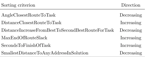
4.2.1 Sorting criteria . . . 27
4.3 Improvement algorithms settings . . . 28
4.4 Size . . . 29
4.4.1 Construction phase . . . 29
4.4.2 Improvement phase . . . 30
4.4.3 Total size . . . 30
4.4.4 Limiting the size . . . 31
4.5 A priori knowledge . . . 31
4.5.1 Analysis . . . 31
4.5.2 Conclusion . . . 32
4.6 Performance landscape . . . 32
5 Tuning method 34 5.1 Tackling general problems . . . 34
5.1.1 Categorical parameters . . . 34
5.1.2 Set of instances . . . 35
5.2 Initial experiment . . . 37
5.2.1 Comparison . . . 39
5.3 Structure of our tuning method . . . 40
5.3.1 Convergence . . . 40
5.3.2 Initial incumbent configuration . . . 41
5.3.3 Building the forest . . . 42
5.3.4 Generating a promising configuration . . . 42
5.3.5 Assessing the promising configuration . . . 43
5.3.6 Limited computation time . . . 45
5.3.7 Multiple objectives . . . 45
6 Experimental results 46 6.1 Modifications . . . 46
6.2 Training and test set design . . . 47
6.2.1 Relevant training instances . . . 48
6.2.2 Training set size . . . 49
6.2.3 Test set . . . 51
6.3 Performance of our tuning method . . . 51
6.3.1 InstanceA. . . 52
6.3.2 InstancesB . . . 53
6.3.3 Conclusion . . . 54
6.4 Performance of our tuned configurations . . . 55
6.4.1 InstanceA. . . 55
6.4.2 InstancesB . . . 56
6.4.3 Conclusion . . . 57
6.5 Versatility . . . 57
6.5.1 Routing benchmark instances . . . 58
7 Conclusions and Recommendations 60
7.1 Conclusions . . . 60
7.2 Recommendations . . . 61
7.2.1 Usage scenarios . . . 61
7.2.2 Other domains . . . 62
7.3 Further research . . . 62
References 64 A Other applications 69 A.1 Forecasting engine . . . 69
Introduction
This research takes place at ORTEC, one of the largest providers of advanced planning and optimization
services. ORTEC’s software products support many types of problems, including, for example, fleet
routing and dispatch, vehicle and pallet loading, workforce scheduling, delivery forecasting, logistics
network planning, and warehouse controlling. In this research, we focus on the solution for routing and
dispatch: ORTEC Routing and Dispatch (ORD). This product supports the process of distributing goods
to customers with a fleet of vehicles. The objective is to minimize the cost of distributing the goods,
while taking into account restrictions and company goals. Instead of delivering goods, also picking up
goods or a mix of delivering and picking up, can be handled by ORD.
ORD bundles the given tasks into routes and adds the right resources (trucks and drivers). This task
is handled by an optimizer, of which two exist for ORD: COMTEC1Distribution Planner Service (CDPS)
and COMTEC Vehicle Routing Service (CVRS). Although they provide basically the same functionality,
differences exist. CDPS is mainly used for solving problems that have a very large number of orders (i.e.,
hundreds to thousands), since it performs significantly faster than CVRS in this case. CVRS is used
for problems in which a large number of restrictions have to be taken into account, which reflects many
practical cases. Our research focuses on the optimizer CVRS.
To optimize the performance of CVRS for a certain customer, its behavior can be influenced by
altering its configuration: a sequence of algorithms, including the parameters of each algorithm, used
to solve the vehicle routing problem. The aim of this research is to develop a method that is able to
systematically find good settings for a given customer. This research is a succession of the recent research
by Van Dijk (2014) at ORTEC, who developed a tuning method for a loading algorithm. This raised
the question at ORTEC whether similar techniques could also be applied to its routing algorithms. The
technique by Van Dijk (2014) is not suitable in this case, due to the reasons we address in Section 1.2.
In this chapter we introduce our research. Section 1.1 provides the context of the optimizer CVRS. We
discuss how this optimizer is working and how we can influence its behavior by changing the configuration.
In Section 1.2, we introduce our problem and break it down in Section 1.3.
1.1
Context
CVRS is an optimization tool for optimizing transport planning. Given a set of tasks (transport orders)
and a set of vehicles, CVRS aims at planning these tasks in those vehicles, while respecting the given
restrictions (e.g., time windows) and optimizing the predefined criteria (e.g., driving distance). This
problem is known as the Vehicle Routing Problem (VRP). CVRS’ primary objective is to plan as many
1ORTECs technical platform common to all its software solutions: a scalable software architecture and application
tasks of the given set as possible. Other objectives can be specified for specific customers, to meet their
wishes. CVRS is designed to assist planners: people that have to solve practical VRPs. CVRS can assist
them in increasing their performance by:
• Speeding up the planning process. CVRS can plan activities much faster than most (experienced) planners.
• Creating planning drafts for the planner to accept or to improve. The planner can use CVRS to create initial plans that could be modified to satisfy these planners’ requirements that are hard to
model.
• Handling complex planning activities (e.g., minimizing costs before minimizing distances, planning routes in areas where the planner is not familiar with, etc.). CVRS can optimize routes under
various criteria and handle planning activities that are outside the capabilities of the planner.
• Optimizing existing routes. The planner can use CVRS to re-optimize existing routes. The sequence of planned tasks within the selected routes will be re-optimized by re-planning the tasks at hand.
• Generate alternatives (proposals) for the planner to choose from. Given a task and a set of routes, CVRS proposes routes in which the task can be planned.
In order to understand the settings that are relevant for CVRS, some background knowledge about the
algorithms used in CVRS is required2. There are two main types of algorithms:
• Construction algorithms, which are used to create an initial solution.
• Improvement (or local search) algorithms, which are used to improve an existing solution.
To construct an initial solution, cheapest insertion is used. After this construction, improvement
algorithms are applied to the initial solution. To influence the behavior of these algorithms, CVRS has to
be configured. Before solving an instance, a configuration has to be specified. This configuration specifies
a sequence of algorithms, including the parameters of each algorithm, used to solve the vehicle routing
problem. A certain configuration is likely to perform different on different problem types. Therefore,
configurations are adapted to make them suitable for the problems of a specific customer (i.e., a sequence
of algorithms and parameter settings that are likely to solve the customer’s problems well). Each of these
algorithms has parameters to control the behavior of the specific algorithm. These parameters can also
be varied to make the configuration even more suitable for a certain customer. There are three main
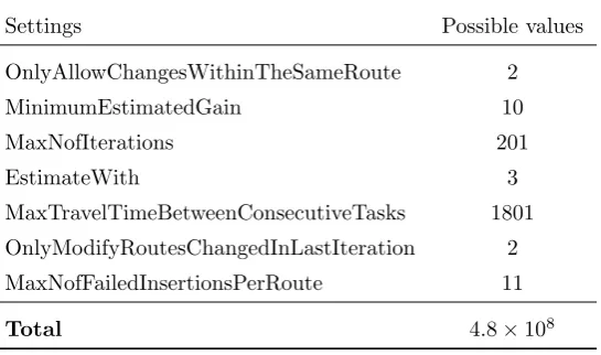
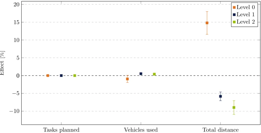
parts, called levels, of the configuration that are highly tunable:
Level 0: The parameters of the construction algorithm For the construction algorithm,
cheap-est insertion, different parameters exist to influence the construction phase. Which parameter
values to use in which case can be specified in the configuration, and could therefore be tuned. The
search space consists of the possible values for the parameters.
Level 1: The sequence of improvement algorithms Within a configuration, we find a sequence
of algorithms used to improve the solution. This sequence can be adapted to align it with the
customer’s situation. This implies that a sequence is chosen that is likely to solve the customer’s
problems well. Different algorithms can be used to improve the solution, e.g., 2-opt, merge and
swap. Which algorithm(s) to use can be specified in the configuration, and could therefore be
tuned. The search space consists of the possible sequences of improvement algorithms.
1 < T e m p l a t e S t r a t e g y=" C o n s t r u c t i o n ">
2 < M a x i m u m B a t c h S i z e v a l u e=" 2 " / >
3 < S o r t i n g C r i t e r i a >
4 < C r i t e r i o n s c a l e=" 0 " d i r e c t i o n=" d e c r e a s i n g " n a m e=" A n g l e C l o s e s t R o u t e T o T r a n s p o r t " / >
5 < / S o r t i n g C r i t e r i a >
6 < C h e a p e s t I n s e r t i o n / >
7 < / T e m p l a t e >
8 < T e m p l a t e S t r a t e g y=" I m p r o v e m e n t ">
9 < 2 O p t E s t i m a t e W i t h=" D i s t a n c e " M i n i m u m E s t i m a t e d G a i n=" 0 " M a x N o f I t e r a t i o n s=" 1 0 0 "
O n l y A l l o w C h a n g e s W i t h i n T h e S a m e R o u t e=" t r u e "/ >
10 < L a r g e N e i g h b o r h o o d M o v e A n d S w a p O n l y M o d i f y R o u t e s C h a n g e d I n L a s t I t e r a t i o n=" f a l s e "
M i n i m u m E s t i m a t e d G a i n=" 0 " M a x N o f I t e r a t i o n s=" 2 0 0 "
M a x T r a v e l T i m e B e t w e e n C o n s e c u t i v e T a s k s I n A G r o u p=" 3 0 0 "
O n l y A l l o w C h a n g e s W i t h i n T h e S a m e R o u t e=" f a l s e " E s t i m a t e W i t h=" D i s t a n c e " / >
11 < 2 O p t E s t i m a t e W i t h=" D i s t a n c e " M i n i m u m E s t i m a t e d G a i n=" 0 " M a x N o f I t e r a t i o n s=" 1 0 0 "
O n l y A l l o w C h a n g e s W i t h i n T h e S a m e R o u t e=" t r u e "/ >
12 < L a r g e N e i g h b o r h o o d M o v e A n d S w a p O n l y M o d i f y R o u t e s C h a n g e d I n L a s t I t e r a t i o n=" f a l s e "
M i n i m u m E s t i m a t e d G a i n=" 0 " M a x N o f I t e r a t i o n s=" 2 0 0 "
M a x T r a v e l T i m e B e t w e e n C o n s e c u t i v e T a s k s I n A G r o u p=" 3 0 0 "
O n l y A l l o w C h a n g e s W i t h i n T h e S a m e R o u t e=" f a l s e " E s t i m a t e W i t h=" D i s t a n c e " / >
13 < 2 O p t E s t i m a t e W i t h=" D i s t a n c e " M i n i m u m E s t i m a t e d G a i n=" 0 " M a x N o f I t e r a t i o n s=" 1 0 0 "
O n l y A l l o w C h a n g e s W i t h i n T h e S a m e R o u t e=" t r u e "/ >
[image:14.595.69.525.93.300.2]14 < / T e m p l a t e >
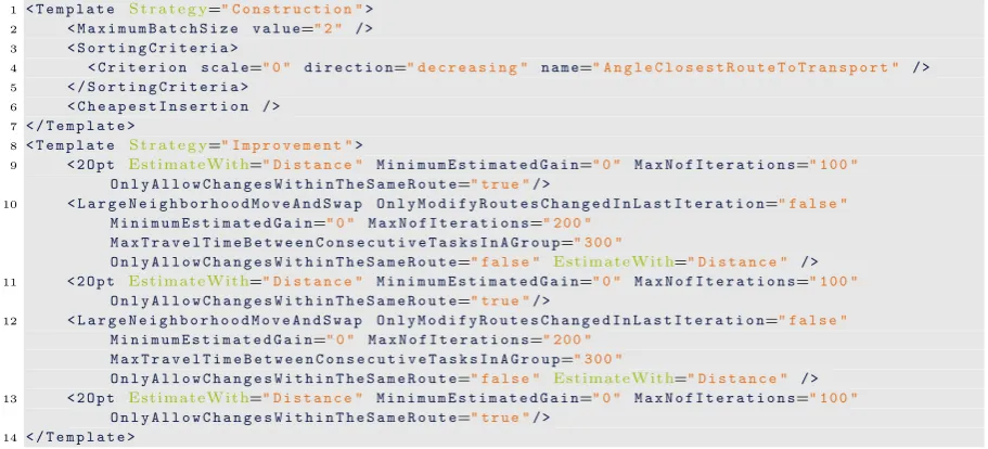
Figure 1.1: Simplified XML representation of the default configuration.
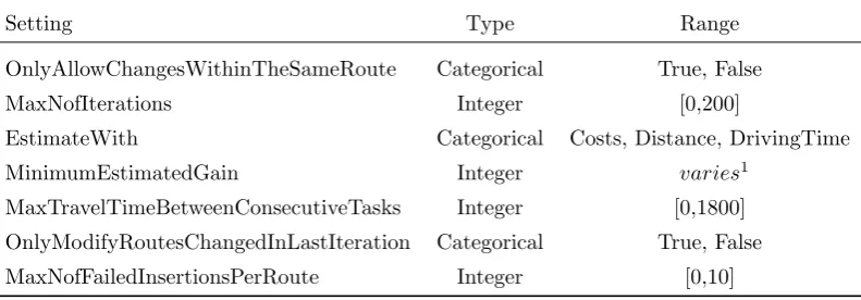
Level 2: The parameters of improvement algorithms A lot of algorithm-specific parameters are
used to control the behavior of the improvement algorithms used. These parameters influence the
trade-off between solution quality and computation time. Which parameter values to use in which
case can be specified in the configuration, and could therefore be tuned as well. The search space
consists of the possible values for the parameters.
The implementation of the configurations is done using so-called command templates. Command
templates are XML files containing information about all three levels. The tuning of these configurations
is currently done manually by the implementation consultants. Figure 1.1 shows an example of the
current default command template.
It is important to note that the optimization tool is deterministic. That is, given a command template
and a problem instance, it always produces the same solution. It has therefore no use to repeatedly solve
a problem instance with the same command template.
1.2
Problem identification
Section 1.1 addressed the tuning options for the configuration in CVRS. Each customer has their own
VRP problems and these problems could differ strongly between customers. We therefore distinguish
different types of customers, grouped by the type of their problem. The optimal configuration is likely to
differ among the problem types. For the same reason, a configuration performs differently for different
customers. That is why configuration tuning is necessary and, at least, type-specific. From experience,
ORTEC knows that the configuration has a large impact on the solution, both its quality and the
required computation time. The need for good configurations is therefore present. However, finding
good configurations is difficult, since it is unclear how a configuration performs for a problem, without
executing (measuring) it. Moreover, measuring the performance of a single configuration on one problem
instance of the customer takes roughly 5 to 15 minutes, which makes finding good configurations also
very time consuming.
The time needed for a measurement, i.e., measuring the performance of a configuration, is the most
important difference between our research and the research of Van Dijk (2014): minutes and seconds
not applicable in our case, due to the tuning time that would be needed.
Tuning the configuration, that is, configuring the routing algorithm, is currently done by the
im-plementation consultants of ORTEC. They manually make tailor-made configurations: configurations
adapted to problems faced by a certain customer. However, this is an undesired situation as it is a
very time (and hence money) consuming task, caused by the facts that the environments differ strongly
between the customers and that configurations are customer-specific. Next to this, there is no empirical
evidence for the performance of the current configurations; they are largely based on the experience of
the consultant. Therefore, ORTEC wants to automate the process of tuning these configurations.
It is important to keep in mind that, since ORTEC operates on many domains, an approach
perform-ing well on many domains, is considered as very valuable. Showperform-ing that a tunperform-ing method performs well
on different domains significantly increases the value of this research for ORTEC.
1.3
Research problem
In this section, we further analyze and break down the problem identified in Section 1.2. First, in
Section 1.3.1, we set the boundaries for our research. Next, in Section 1.3.2, we define our objective, and
in Section 1.3.3 we clearly state our problem. We end this section with the research questions that guide
our research.
1.3.1
Scope
The tuning method we want to develop has to operate within a certain context, whose boundaries we
describe in this section.
To tune the configurations, we use the available improvement methods and parameters. We do not
seek to develop new improvement methods, but limit ourselves to the currently implemented, and
there-fore useable, methods. Besides, we do not want to introduce new parameters, but stick to the currently
available set of parameters. Summarized, we want to take full advantage of the current framework
(CVRS) by deploying it with the best possible configuration for a certain customer.
We consider the time required to solve a problem instance as expensive, since it is the time a planner
has to wait. We denote this time as the computation time. Currently, the configurations are tuned offline:
not while solving a problem instance, but beforehand at moments when an abundance of computational
resources is available. Therefore, tuning does not add to the computation time. We use a set of training
instances that are similar to future, unseen instances. This is needed since the configuration is an input
for CVRS, just as an instance of the problem. Another option might be to tune the configuration
while solving the problem, known as online tuning. In this case, tuning does add to the computation
time. As a result, solving the problem with online tuning requires more computation time compared
to solving the problem with offline tuning. Combined with the desire to keep the computation time for
the customer at a minimum, offline tuning seems to be more appropriate. This is also supported by the
design of CVRS, because of its need for a pre-defined configuration. If online tuning would have been
suitable for the problem instances solved with CVRS, a pre-defined configuration would not have been
necessary. However, we review methods for both variants, since it is likely that we can adapt, or use
logic incorporated in online tuning methods to make them suitable for offline tuning.
A first exploration of the currently used command templates does not give a strong indication about
which level (see Section 1.1) of the configuration is most suitable for tuning. Since level 0 influences
the way the initial solution is created, we expect a significant impact of the parameters on this level.
In addition, our intuition says that changing the order of the sequence of the algorithms, level 1, has
evidence for this thought, we do not focus on a level right now. On the contrary, we try to develop a
method that is able to address the tuning of all three levels. We notice some common patterns in the
command templates, which indicates that certain combinations perform well. We take this into account
when searching for and developing a new tuning method.
For our research, we have access to a single VRP instance of one of ORTEC’s customers with 224
tasks. These tasks are spread over Western Europe and 23 vehicles are available for transporting them.
From now on we refer to this VRP instance asinstanceA. In addition, we have a set of 5 VRP instances
of another customer of ORTEC. Each instance represents one day and contains about 1000 tasks. Each
day, 10 vehicles are available. From now on we refer to these VRP instances as instancesB. Using
these instances we are able to perform experiments and validate our tuning method. Due to the time
restrictions of this research, we were not able to perform experiments with more (sets of) instances.
Unfortunately, it is not possible to use benchmark instances with the software, such as the well-known
Solomon (Solomon, 1987) instances.
1.3.2
Objective
The main objective of this research is to design and implement a method, able to automatically configure
the routing algorithms to optimize their behavior on future instances. By this, the time-consuming
manual tuning of the configuration will be reduced to a minimum. The quality of the solution should at
least be comparable with the current quality. The computation time depends on the chosen configuration,
since it specifies when to stop improving the solution (see Chapter 4). However, this is not based on time
but on the state of the solution. The computation time with the tuned configuration should not exceed
15 minutes, since planners do not want to wait any longer (unless it significantly improves the quality
of the solution). Hereby we discard the computation time needed to create a good configuration using
our tuning method, since this is only done periodically, at moments with an abundance of computational
resources. However, for practical reasons we do not want to spend more than a weekend (i.e., about 60
hours) on tuning. If we do not meet the given requirements, customers are likely to prefer the current
configurations.
1.3.3
Problem statement
The optimization tool CVRS needs a method to automatically configure the routing algorithms to
opti-mize their behavior on future, unseen instances. This, so-called, algorithm configuration problem can be
defined as follows: “given a parameterized algorithm A, a set of problem instancesI, and a cost metric
c, find parameter settings of Athat minimizec onI” (Hutter et al., 2011).
1.3.4
Research questions
We formulate a number of research questions to achieve our research objective in a structured manner.
First, in Chapter 2, we introduce the VRP problem by exploring the comprehensive collection of solution
methods for VRPs by means of a literature study. Maybe some of these methods would fit within our
framework. However, most of the methods are not likely to be able to tune the configuration, since this
would require a structural change to our framework (e.g., adding improvement methods or parameters).
Afterwards, we therefore review methods that are able to tune configurations.
1. What literature is available related to vehicle routing problems and tuning configurations?
(a) What solution methods are available for VRPs?
Second, in Chapter 3, we want to analyze how the optimizer CVRS solves VRPs by using it and reading
the manual. This helps us in understanding the impact of different configurations.
2. How does the optimizer CVRS solve VRPs?
Third, in Chapter 4, we want to analyze the configuration possibilities of CVRS. We discuss to what
extent we can tune the configurations. In Section 1.2 we introduced the issue related to different types
of problems. Our aim is the find a priori knowledge (e.g., algorithms that are suitable for a certain type
of problem) that we can incorporate in our new tuning method. Here we use the experience of ORTECs
experts. We also explore our performance landscape and look at the effect of various parameters.
3. What are the characteristics of our search space?
(a) To what extent can we tune the configurations?
(b) What useful information can we find in tailor-made configurations?
(c) How does our performance landscape look like?
Fourth, in Chapter 5, we want to develop a tuning method that tunes the configuration by combining
the knowledge obtained during our literature study as well as our exploration of the configuration.
4. What tuning method can we develop to automatically tune the routing algorithms?
Fifth, in Chapter 6, we want to test the performance of our new tuning method in various ways: (i) by
comparing our method for tuning routing algorithms with alternative tuning methods, (ii) by comparing
the tuned configurations with the configurations currently used, and (iii) by testing how the method
performs on other problem domains (since ORTEC values general approaches, as mentioned in Section
1.2). To make this possible, we integrate the tuning method with CVRS.
5. How well does our new method perform?
(a) How well does our new tuning method perform compared with alternative tuning methods?
(b) How well do the configurations created with our new tuning method perform compared to
other configurations?
(c) How well does our new tuning method perform for other ORTEC products?
Finally, in Chapter 7, we want to present the conclusions and recommendations. We want to discuss
how ORTEC can use our new tuning method in practice, such that its customers benefit from it. By
discussing with ORTECs experts we find the best manner.
6. How can ORTEC implement our new tuning method?
Literature review
This chapter gives an overview of the literature about vehicle routing problems and configuration tuning.
We start with a overview of methods that are used to solve vehicle routing problems in Section 2.1. Next,
in Section 2.2, we address techniques that are used in the field of configuration tuning.
2.1
Vehicle routing problems
Over 50 years ago, Dantzig and Ramser (1959) introduced The Vehicle Routing Problem (VRP) asThe Truck Dispatching Problem. It is a combinatorial optimization problem in which a number of customers has to be serviced with a fleet of vehicles given a set of constraints, while minimizing the total route cost.
Many companies face this problem on a daily basis, for example if the supplying of supermarkets has to
be planned.
Each VRP instance typically consists of many constraints, such as time windows, precedence
rela-tions, and vehicle capacity. Therefore, many variants of the VRP exist. However, a lot of research has
concentrated on the classical VRP, a basic variant of the problem which can be adapted to meet real-life
situations by adding restrictions.
The most common definition of the classical VRP is as follows. Let G = (V,A) be an undirected graph where V ={0,1, . . . ,n} is the vertex set andA={(i,j) : i,j ∈V, i̸=j} is the arc set. Vertex 0 represents the depot, wheremvehicles of capacityQare located. The other vertices represent customers. Each customer i∈V \ {0} has a non-negative demandqi ≤Q. A cost matrixcij is defined onA. The
problem consists of determining a set of at mostmvehicle routes such that (i) each route starts and ends at the depot, (ii) each customer is visited exactly once by exactly one vehicle, (iii) the total demand of
each route does not exceedQ, and (iv) the total routing cost is minimized.
The VRP is a generalization of the Travelling Salesman Problem (TSP). In a TSP, the goal is to find
the shortest route from an origin, to each of the cities of the problem, and back to the origin.
We start with a discussion of the different variants of the VRP in Section 2.1.1. In Section 2.1.2 we
explore the wide field of solution methods for VRPs.
2.1.1
Variants
The classical VRP does, in many cases, not reflect the real-life situation as a lot of constraints are missing.
Capacity constraints were already included in the classical VRP but other common constraints include
(Laporte, 1992):
• Time windows: locationimust be visited within the time interval [ai, bi] and waiting is allowed at
with Time Windows (VRPTW).
• Precedence relations between pairs of locations: location imay have to be visited before location
j. An example is the pickup of an order at location i which should be delivered at location j by the same vehicle, known as the Vehicle Routing Problem with Pickup and Delivery (VRPPD).
• Driving time restrictions: due to drivers’ legislation, drivers have to comply with rules on driving time, breaks, and rests.
A dynamic VRP (DVRP), which may include any of the above constraints, is a VRP that can change
while solving the problem. Traffic jams or unexpected arrivals as well as cancellations of orders are
examples of such changes.
A typical, practical VRP instance contains several constraints of different types (e.g., time windows
and precedence relations). Since the aforementioned abbreviations are insufficient in those cases,
prob-lems with many types of practical constraints are called rich VRPs. Most practical instances are therefore
rich VRPs.
2.1.2
Solving VRPs
The VRP is a NP-hard problem for which it is hard to determine sharp lower bounds on the objective value
(Cordeau, Gendreau, Laporte, Potvin, & Semet, 2002). Exact algorithms using implicit enumeration will
therefore converge slowly, which makes them incapable of solving realistic problem sizes with a constant
success rate in an acceptable time. The best known exact algorithms are able to handle approximately a
hundred vertices (Baldacci, Christofides, & Mingozzi, 2008), but real instances often exceed this size. As a
consequence, research has focused on heuristics (Laporte, 2007). Heuristics are also easier to adapt (e.g.,
adding restrictions), which is needed in order to meet real-life situations. The dynamic programming
heuristic by Kok, Meyer, Kopfer, and Schutten (2010), for example, takes the full European social
legislation on drivers’ driving and working hours into account. Nevertheless, solution methods for rich
VRPs are scarce.
To structure the remainder of this section, we use the classification of solution methods for the VRP
by Laporte (2007) as a guideline. First, we review conventional methods, divided into exact algorithms
and classical heuristics. With the term “classical” we refer to heuristics that do not allow the objective
function to deteriorate in a consecutive iteration. Heuristics that do allow this, are described later in
this chapter, and we call them metaheuristics. Both classical heuristics and metaheuristics search within
a search space of problem solutions. The so-called hyper-heuristics, on the other hand, search within a
search space that contains heuristics. For this reason, we address them in Section 2.2, where we discuss
configuration tuning methods.
Exact algorithms
Exact algorithms exist to solve the VRP, but their success in solving realistic instances with larger size is
limited. Direct tree search methods, dynamic programming, and inter linear programming are the three
main types of methods within this category.
Direct tree search Direct tree search methods solve the VRP by sequentially building routes by using
a branch and bound tree. Christofides and Eilon (1969) developed one of the first algorithms using a
direct tree search method. Their algorithm branches on arcs, and branches are created by either including
or excluding an arc in the solution. Later, Christofides (1976) developed a branch and bound algorithm
easy or small instances could be solved with these algorithms. The introduction of two methods that
were able to derive sharp lower bounds (Christofides, Mingozzi, & Toth, 1981) considerably enhanced the
performance of these algorithms. Fisher (1994) used this knowledge as well, which resulted in a method
able to solve an instance with 71 customers.
Dynamic programming Dynamic programming (DP) is an optimization approach that can solve
complex problems by dividing them into a sequence of simpler sub-problems. These sub-problems are
solved in multiple stages so that in each stage a part is added to the partial solution. In the last
stage, the optimal solution is found. The following DP algorithm is based on the DP formulation for
the Traveling Salesman Problem by Held and Karp (1961). Let V be a set of nodes representing all customer locations with 0 being the departing node (e.g., the depot). Given S ⊆ V \ {0} and i ∈ S, letC{S,i} be the cost of the best route that starts in node 0, visits all nodes in setS and ends in node
i. Then the recurrence relation isC(S,i) =c0i forS ={i} andC(S,i) =minj∈S\{i}[C(S\ {i},j) +cji]
for S otherwise. The second part of the recurrence relation can be explained as follows. Consider the shortest path from node 0 to nodei, visiting all nodes from S\ {i} which has nodej ∈S immediately preceding node i. Since the nodes in S \ {i} are visited in optimal order, the length of this path is
C(S\ {i},j) +cji. By taking the minimum over all choices ofj we obtain the minimum ofC(S,i). The
ultimate goal is to find the minimum cost of a complete tour, terminating in node 0, which is given
byC(V,0) =mini∈V\{0}[C(V \ {0},i) +ci0]. In each stage, the partial solutions are extended with an extra node. The number of stages is the number of nodes that are available in DP. Each stage can have
multiple states, which are partial solutions of the main problem. The discussed DP algorithm creates
only one route and applying it to the VRP is therefore not straightforward. Gromicho, van Hoorn, Kok,
and Schutten (2012) use the giant-tour representation (GTR) of vehicle routing solutions to apply the
approach to the VRP. In a GTR all routes are connected such that they form one giant route. By this,
the VRP is transformed into a sequencing problem. This makes it possible to use the DP formulation of
the TSP to solve it. The framework of Gromicho et al. (2012) ensures that the DP solution of the GTR
is feasible for the original VRP.
Integer linear programming Most research on exact algorithms for the VRP has been done in the
field of integer linear programming (Laporte & Nobert, 1987), which has resulted in variety of methods
in this category. Vehicle flow formulations are by far the most widely used among the integer linear
programming (ILP) methods. Variables indicating how many times edge [i,j] appears in the solution are used in the two-index variant by Laporte, Nobert, and Desrochers (1985). The three-index variant adds
the vehicle making the route to this variable (xijk) (Fisher & Jaikumar, 1978).
Set partitioning formulations, first suggested by Balinski and Quandt (1964), are rarely used in
practice because of their large number of variables. However, the most successful VRP algorithms
partially use a set partitioning formulation (Laporte, 2009). Examples of such algorithms are found in
Fukasawa et al. (2006) and Baldacci et al. (2008).
Commodity flow formulations, such as the two-index two-commodity flow formulation for the
capac-itated VRP by Baldacci, Hadjiconstantinou, and Mingozzi (2004), use additional variables for both the
vehicle load on an edge and the remaining capacity of the vehicle travelling on an edge. The authors
show that this formulation allows to solve instances up to 100 customers, although with mixed success.
Classical heuristics
Classical heuristics can be subdivided into two categories: construction heuristics and improvement
depot starting line
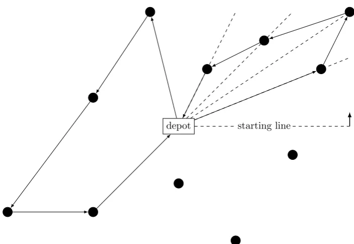
Figure 2.1: An example of the sweep algorithm, in which the capacity of a vehicle is 4 customers and the sweep direction is counter-clockwise.
initial, feasible solution whereas improvement heuristics do start with a feasible solution which they try
to improve.
Construction The most well-known construction heuristic to solve a VRP is probably the saving
algorithm by Clarke and Wright (1964). The main idea is to merge routes based on the generated savings
by this merge. Initial routes are constructed from the depot to the customer and directly back to the
depot (so one customer per route). Next, the algorithm calculates the possible savingssij =ci0+c0j−cij
by removing the arcs (i,0) and (0,j) and adding the arc (i,j), if this results in a positive saving and a feasible merged route. The merge yielding the largest saving is implemented. This process iterates until
profitable and feasible savings are not possible anymore. The simple implementation of this heuristic and
the ease with which additional restrictions can be added explains its popularity. Several improvements to
the saving algorithm have been proposed. Gaskell (1967) and Yellow (1970) try to create more compact
routes by adding a positive parameterλto savings formulation: sij =ci0+c0j−λcij. The enhancement
of Altinel and ¨Oncan (2005) uses a modified savings function that includes the customer demands impact.
Another well-known heuristic is the sweep algorithm by Gillett and Miller (1974). Starting with a
line rooted at the depot, it sweeps this line either clockwise or counter-clockwise. Customers that are
encountered while sweeping this line are added to the route. A new route starts once it is infeasible
to include the next customer to the current route, for example because of capacity restrictions of the
vehicle. Figure 2.1 visualizes the algorithm. This method makes sure that only non-intersecting routes are
generated. This method is a so-called cluster first, route second method. These methods are characterized
by the fact that they first form groups of locations, clusters, and try to build a route based on these
clusters afterwards.
Fisher and Jaikumar (1981) presents an algorithm that consists of two phases. First, seed points (i.e.,
points that will end up in disjoint routes) are chosen and customers are divided in clusters by solving
a generalized assignment problem (GAP). How to determine these seed points is not made clear in the
original article, but some articles address this issue (Bramel & Simchi-Levi, 1995 and Baker & Sheasby,
CVRS uses cheapest insertion, based on the sequential insertion heuristic by Solomon (1987), as its
construction heuristic. Routes are initialized with a seed location, selected by, for example, the location
farthest away from the depot. The remaining locations are added at the cheapest insertion point in the
route constructed so far, until the route is full (e.g., capacity constraints). The insertion cost is defined
ascik+ckj−cij for an insertion of location k. This process repeats until all locations are serviced.
Improvement Improvement heuristics take a feasible route as a starting point. Then, they try to
improve the route by either (i) intra-route or (ii) inter-route changes. Intra-route heuristics switch the
position of one or more customers within a route; inter-route heuristics move one or more customers
between different routes.
The 2-opt heuristic by Croes (1958) is an intra-route improvement method that generates a 2-optimal
route: a route that cannot be shortened by exchanging two arcs. This is achieved by removing crossings
(arcs that intersect) from routes, as crossings are never optimal in the classical VRP with symmetric
cost matrix. However, because of, for example, time-windows, the optimal route could contain crossings
in other VRP variants. A related method is Or-opt (Or, 1976), where a number of consecutive vertices
are relocated while maintaining the orientation of the original route.
Thompson and Psaraftis (1993) describe a b-cyclic,k-transfer scheme in which b routes are selected for a circular permutation and for each routekcustomers are moved to the next route of the permutation. Computational experience shows that combinations of b = 2 or b = variable and k = 1 or 2 seem to produce good results. Slightly modified approaches of this idea are used in the improvement phase of
CVRS.
Numerous other inter-route improvements heuristics have been developed, including ejection chains
(Glover, 1992), GENI (Gendreau, Hertz, & Laporte, 1992), λ-interchange (Osman, 1993), and CROSS (Taillard, Badeau, Gendreau, Guertin, & Potvin, 1997).
Metaheuristics
The exploration of the solution space is much more thorough within metaheuristics compared to classical
heuristics. Within metaheuristic, moves that are inferior or infeasible can also be accepted in order to
escape from local minima. Three main categories exist within this field: (i) local search, (ii) population
search, and (3) neural networks.
Local search Local search methods are methods that explores the neighborhood of the current solution
and moves each iteration to a solution in that neighborhood. Different types of methods exist within
this category to define and explore neighborhoods.
Tabu search methods remember properties of previously visited solutions and make sure that those are
not considered again in subsequent iterations. A metaheuristic based on this approach is TABUROUTE,
developed by Gendreau, Hertz, and Laporte (1994). This algorithm uses neighborhoods that are found
by “repeatedly removing a vertex from its current route and reinserting it into another route”. They also
allow intermediate infeasible solutions to escape from local minima, which is not common for tabu search
methods. Taillard (1993) presents an approach that decomposes a VRP into independently solvable
subproblems. This speeds up the applied iterative search method, in their case tabu search. The
strengths of the unified tabu search algorithm (UTSA) by Cordeau, Laporte, and Mercier (2001) lie in its
flexibility and robustness. Using a simple exchange procedure, controlled by tabu search, neighborhoods
are explored and good quality solutions are found. Toth and Vigo (2003) propose a granularity concept.
Long edges (i.e., edges with a length exceeding a certain threshold) are never considered by the search
Another branch of local search metaheuristics is based on variable neighborhood search. Here, the
algorithms try to find local optima, and switch to another neighborhood once a local optimum is reached.
The two-phase variable neighborhood search heuristic by Kyt¨ojoki, Nuortio, Br¨aysy, and Gendreau (2007) uses a variable neighborhood search scheme to guide the improvement heuristics. Other applications of
variable neighborhood search to the VRP are the two-stage hybrid algorithm by Bent and Van Hentenryck
(2004) and a very-large scale neighborhood search algorithm by Ergun, Orlin, and Steele-Feldman (2006).
A well-known heuristic based on variable neighborhood search is the heuristic by Pisinger and Ropke
(2007). We discuss this heuristic in Section 2.2.1, since it is strongly related to configuration tuning.
Population search Population search methods, such as genetic algorithms (Holland, 1975), simulate
the process of natural selection. By mutating the properties of candidate solutions from a population
of solutions, the population evolves towards a new generation consisting of hopefully better solutions.
Baker and Ayechew (2003) applied this method to the classical VRP problem. Their results show that
the method can be competitive with other heuristics, both in computation time and solution quality.
Often genetic algorithms are combined with local search, as described by Rochat and Taillard (1995),
Mester and Br¨aysy (2007), and Vidal, Crainic, Gendreau, and Prins (2014).
Ant colony optimization has received a lot of attention for VRPs. These methods are based on the
behavior of ants. Edges that appear frequently in good solutions are remembered as good edges and
they are more likely to be included in other solutions. Early attempts based on these ideas applied the
method to the classical VRP (Bullnheimer, Hartl, & Strauss, 1999), and their promising results led to
ant colony optimization methods for variants of the classical VRP (Gambardella, Taillard, & Agazzi,
1999).
Many other population search methods exist, such as genetic programming or evolution strategies,
but they are not noteworthy in the light of the VRP, since, to our knowledge, they have not been applied
successfully.
Neural networks Neural networks mimic the way biological neural systems, such as the brain, operate.
This concept has only received little attention in the context of vehicle routing. Ghaziri (2004) and
Schumann and Retzko (1995) have both applied self-organizing maps, a type of neural network, but they
have not been able to find good solutions in an efficient way. The same holds for the approach of Potvin
and Robillard (1995). To our knowledge, this line of research has received little attention in recent years.
Combined with the unsuccessful early attempts, it is plausible that the opportunities of neural networks
for the VRP are limited.
2.1.3
Conclusion
Exact algorithms are not applicable for our research as none of the described methods is able to solve
instances of a realistic size, especially not with our limitations on computation time. As a result, we
focus on heuristic approaches, which are currently used by CVRS.
The classical heuristics require low computational effort, but they are incorporating many restrictions
is complicated. This makes them unappealing for practical situations in which numerous side constraints
exist.
Metaheuristics are more flexible, which makes them more useful in practice, but this is done at the
expense of computation time. None of the metaheuristics described in our review are solely based on
simple heuristics as we have in our framework. Instead, they are mostly tailor-made for a specific VRP
Feedback Nature of the heuristic search space
Heuristic selection
Construction heuristics
Online learning
Hyper-heuristics
Perturbation heuristics
Offline learning
Heuristic generation
Construction heuristics
No learning
[image:24.595.73.526.82.247.2]Perturbation heuristics
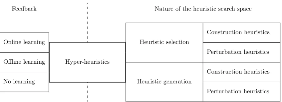
Figure 2.2: A classification of hyper-heuristic approaches (Burke et al., 2010).
Summarized, none of the discussed methods strongly resembles our complete framework, making
them unsuitable to solve our problem.
2.2
Configuration tuning
As mentioned before, we have three levels in the configuration to tune. First, we discuss methods to tune
the sequence of our improvement algorithms, which we called level 1. Therefore we need methods that
use a search space of heuristics rather than solutions (as metaheuristics do). Applicable literature can
be found in the field of hyper-heuristics, which we discuss in Section 2.2.1. Second, we discuss general
tuning methods, which can be applied to all levels, in Section 2.2.2.
2.2.1
Hyper-heuristics
A hyper-heuristic is defined as “an automated methodology for selecting or generating heuristics to solve
hard computational search problems” (Burke et al., 2010). This research field arose from the need to
raise the level of generality at which search methodologies can operate. This term was first used in the
context of combinatorial optimization to define “heuristics that choose heuristics” (Cowling, Kendall,
& Soubeiga, 2001). In this context, hyper-heuristics operate on a search space of low-level heuristics.
Low-level heuristics are generally widely known heuristics that are able to solve (parts of) VRPs, such
as those discussed in Section 2.1.2. From this, given a particular problem instance, they select and
apply suitable heuristics. This seems to fit with our need for a method that selects appropriate low-level
heuristics, given the problem instance at hand.
Burke et al. (2010) propose a classification for hyper-heuristics, which we will use to structure our
discussion on hyper-heuristics. Their classification uses two dimensions: (i) the nature of the heuristic
search space, and (ii) the source of feedback during learning.
From the definition of a hyper-heuristic, we conclude that there are two categories of hyper-heuristics:
heuristic selection and heuristic generation. Figure 2.2 shows that both categories are also present in
the proposed classification. We therefore consider these two categories as the most fundamental, and the
remainder of this section is structured along these.
Figure 2.2 provides us with more information about the different types of hyper-heuristics. Within
both heuristic selection, and heuristic generation, we find another categorization. This categorization
concerns the nature of the search space (i.e., the type of low-level heuristics), namely between
Section 2.1.2). Methods based on construction heuristics build their solution incrementally: an empty
solution gradually evolves to a complete solution by intelligently selecting and applying construction
heuristics from a pre-defined set. On the other hand, methods based on perturbation heuristics do not
start with an empty solution. They aim to improve a candidate solution by selecting and applying
pertur-bation heuristics in a clever way. Hyper-heuristics may also consider both construction and perturpertur-bation
heuristics. We label these as hybrid methods.
The other dimension, the source of feedback, concerns the learning mechanism. This describes the
way feedback from the search process is used. In this classification, we find three groups: (i) online
learning, (ii) offline learning, and (iii) no learning. The first group comprises methods that learn while
solving an instance of a problem. Here feedback is received during the search process of a specific
instance. Therefore, instance-specific properties can be taken into account, resulting in a selection of
low-level heuristics that is tailor-made for the problem instance. On the other hand, offline learning
approaches use a set of training instances. These training instances should be representative for other
unseen problem instances of the same type. The idea is to gather knowledge for a generalized problem
of a particular type to develop a heuristic that, hopefully, performs well on any instance of the same
type. Obviously, the latter group, no learning, does not use any feedback. In this case, choices are made
based on predetermined rules that do not depend on knowledge gathered in previous iterations (e.g.,
randomly).
From the previous paragraph, we conclude that using hyper-heuristics does not, implicitly, make a
choice between online or offline tuning either: a hyper-heuristic could use either method. In our case,
we tune offline, as stated in Section 1.3.1. However, we might be able to use some logic incorporated in
online tuning methods. Here it is important the keep a structural difference between online and offline
tuning methods in mind. As introduced in Section 1.3.1, the time an online tuning method needs is
part of the computation time for a problem instance. As a consequence, online tuning methods typically
focus on parts of the search space that are likely to perform well. By this, the risk that time is spent on
measuring bad performing configurations is reduced. For offline tuning methods, the tuning time does
not add to the computation time. Offline tuning methods can afford to measure configurations in parts
of the search space where the performance is still unknown, to reveal the performance landscape in these
areas. Since we opt for offline tuning, we have the opportunity to explore unknown parts of the search
space. If we (partly) use online methods, we must ensure that we do not focus on known parts of the
search space only.
We continue this chapter with a discussion of examples (in the application domain of vehicle routing,
if possible) of heuristic selection methods and heuristic generation methods. For an exhaustive survey,
we refer to Burke et al. (2013).
Heuristic selection methods
Heuristic selection methods solve a problem by choosing promising combinations of existing low-level
heuristics, both construction and perturbation heuristics.
Among the heuristic selection methods (partly) based on construction heuristics, we find a
hill-climbing based hyper-heuristic by Garrido and Castro (2009). Hill-hill-climbing is a local search method in
which incremental changes to an initial solution are made until no further improvements can be found.
A collaborative framework chooses a combination of simple low-level heuristics, based on the nature of
the problem at hand (online learning). It is a hybrid method since it considers both construction and
perturbation heuristics. Tests of the method on the CVRP show that this method delivers stable and good
quality solutions for various types of problems. This implies that the framework is able to adapt itself to
evolutionary hyper-heuristic is proposed (Garrido, Castro, & Monfroy, 2009). This hyper-heuristic is very
similar, also in terms of performance on the CVRP, to the previously mentioned hill-climbing based
hyper-heuristic. Garrido and Riff (2010) use the idea of an evolutionary hyper-heuristic to solve the DRVP.
To be able to take the unexpected changes that might occur in a DVRP into account, they introduce
a third type of low-level heuristic: noise heuristics. Again it achieves competitive results. Finally,
HyperPOEMS (Mlejnek & Kubal´ık, 2013) is an improved evolutionary hyper-heuristic. An
evolutionary-based iterative search algorithm controls the process of autonomously searching suitable combinations of
low-level heuristics for a particular problem instance. Results indicate that it outperforms the previously
mentioned hyper-heuristics for the CVRP. Although the aforementioned hyper-heuristics are, at least
partly, based on construction heuristics, the main idea could still be used in our case as the effect of the
order of the sequence is taken into account here.
Pisinger and Ropke (2007) present a method that is based on perturbation heuristics. In their
adaptive large neighborhood search (ALNS) “a number of simple algorithms compete to modify the
current solution”. In each iteration a perturbation heuristic, consisting of one algorithm to destroy and
one algorithm to repair the current solution, is chosen. An adaptive layer that uses roulette wheel
selection, makes this choice, based on the low-level heuristics performance during previous iterations, so
it learns online. A local search framework (e.g., simulated annealing or tabu search) decides whether or
not to accept the new solution, created by the chosen heuristics. The generality of the ALNS framework
makes it possible to use the method for a wide spectrum of VRPs. The fact that the method was able
to improve several well known solutions of benchmark instances, shows that it is promising. However,
the framework does not take the sequence of the heuristics into account. Therefore the effect of the
order of the sequence, which we consider as important, is neglected. The coalition-based metaheuristic
(CBM) by Meignan, Koukam, and Cr´eput (2010) is a self-adaptive and distributed metaheuristic. Several
agents concurrently modify the solution by choosing a low-level heuristic. The selection of a heuristic is
adapted dynamically using learning mechanisms, which are applied during the optimization. To assess
the performance of CBM, experiments on the VRP have been conducted. This shows that the heuristic
is competitive with powerful heuristics.
Heuristic generation methods
Heuristic generation methods tackle a problem by searching and selecting from a space of basic
building-blocks of heuristics. These building-building-blocks are obtained by decomposing heuristics into their basic
com-ponents. Heuristic generation methods return, next to the solution, a reusable heuristic that can be used
to solve similar yet unseen problems. At first sight this seems to fit perfectly with our problem and the
desired solution, as we can consider our improvement algorithms as components of our configuration (our
complete improvement algorithms).
To our knowledge, only a few attempts have been made to apply a heuristic generation method to the
VRP. These efforts take a grammatical evolution (GE) (O’Neill & Ryan, 2001) approach. GE is related
to genetic programming: it is an evolutionary algorithm that can evolve complete programs. Drake,
Kililis, and ¨Ozcan (2013) propose a GE hyper-heuristic that evolves components of the well-studied
metaheuristic VNS. Sabar, Ayob, Kendall, and Qu (2013) present a framework that uses GE, “which
takes several heuristic components as inputs and evolves templates of perturbation heuristics”. Although
both methods are categorized as heuristic generation methods, neither reuses the generated heuristic on
other instances of the same type. Instead, the heuristic is applied for each instance individually, making
it hard to predict if the generated heuristic is suitable for reuse.
In other application domains we find methods that generate heuristics, which are thereafter tested
problem that produces good quality perturbation heuristics. Only one training instance is used in
the offline learning process, which is used for the evolution of the heuristic. Still, each run on the
training instance(s) generates a new, and possibly different, heuristic. This set of heuristics maintains its
performance on new problem instances for the same type, i.e., they are appropriate for reuse. A method,
to choose the most suitable heuristic for the problem type out of this set, is not provided. The difference
in computation time for one iteration in the case of Burke et al. (2012) and our case differs strongly, less
than a second and 5 to 15 minutes respectively. In the bin packing case, hours of tuning were needed
to find a suitable solution. As it seems plausible that a comparable part of the search space should be
measured in our case. As a consequence, it would take weeks to find a feasible solution in our case.
Although we did not restrict the time for offline tuning, weeks is obviously too long for the scope of this
research. Other methods are largely based on genetic programming as well, making them unsuitable as
well given the issues with tuning time that will occur.
Conclusion
We discussed several methods to tune the sequence of the algorithms in the configuration. In general,
the methods choose the most applicable low-level heuristic out of a set of low-level heuristics, based on
the nature of the problem on hand. To achieve this, most methods use online learning. However, some
methods seem to be able to make them applicable for offline tuning by slightly modifying them (as we
already expected).
In general, the heuristic selection methods use online learning mechanisms. The use of a certain
low-level heuristic differs between different problem types. We might therefore be able to apply the
methods as offline tuning methods, and use the results for problem instances of the same type. Since
these methods produce sequences of heuristics for a particular problem instance, we would likely end
up with many different sequences. Therefore, we would have to solve the difficult problem of creating
the most promising sequence out of a large set of sequences (evolved from all instances of the training
set). We could simplify this problem by selecting, instead of creating, the most promising sequence.
By enumerating all sequences for all instances, we could then select the sequence that performs best on
average. However, it is far from certain that the sequence we select in this case, is a good sequence on
average. That is, we might have found a completely different, better sequence if we aimed at creating a
single sequence for all instances. This approach seems therefore unsuitable.
The use of a heuristic generation methods seems more appropriate. Several methods show that the
generated heuristics are indeed suitable for reuse. However, none of the methods develops one heuristic
per problem type. Instead, they provide a set of heuristics that, individually, perform well on a certain
problem type. If we would use these methods in our case, we have to find the most suitable heuristic
of this set. We end up with the same problem as for heuristic selection methods. In addition, these
methods would require weeks of computation time, which does not suit this research.
We could adapt the before mentioned methods to align them more with our needs, for example by
using methods that are able to choose the most promising heuristic out of the created set. Nevertheless,
hyper-heuristics are generally used for problems with a much smaller search space. It is therefore likely
that the computation time exceeds our limits. Moreover, tuning the settings of the algorithms (level 2)
is not addressed with these methods, so we would need an additional method. As a consequence, we
would have to combine these methods, which could be complicated as well.
2.2.2
Automated tuning methods
Different configurations typically result in different solutions, so tuning them has a high likelihood of
is time-consuming and hard to do by hand, automation is very likely to be beneficial.
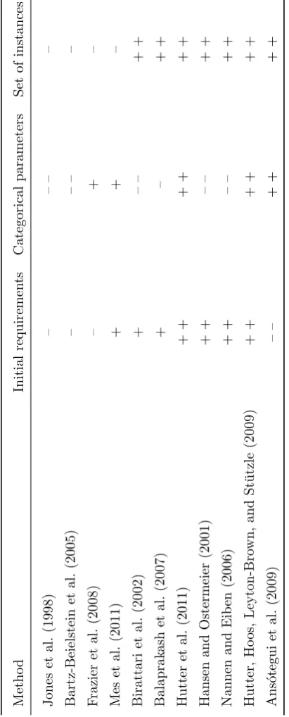
Parameters can be divided into two categories: numerical and categorical. The distance between
numerical parameter values can be used as a metric, but this is not possible for categorical parameter
values. In the case of tuning numerical parameters, this metric is used to guide the search. Categorical
parameters are more difficult to tune, as many samples are required to spot parameter superiority
(Dobslaw, 2010). Assessing this distinction is therefore important and we will take it into account in our
discussion.
Based on Hutter, Hoos, Leyton-Brown, and St¨utzle (2009), we define our problem as follows. Let
A(θ,Π) be the algorithm we want to optimize, with its parametersp1, . . . ,pk that returns the objective
value for a minimization problem. Θi is the domain, i.e., the possible values, for each parameterpi. The
space of all possible configurations is denoted by Θ ⊆Θ1× · · · ×Θk. The quality of the configuration
θ∈Θ isA(θ,Π), which is a deterministic quality measure, which depends on the problem instanceπon hand. We denote the training set by Π. We aim to find the optimal configurationθ∗∈argminθ∈ΘA(θ,Π). Unfortunately, no universally applicable tool to solve this problem exists, but recent developments
have led to significantly improved methods (Dobslaw, 2010). In general, but especially in our case, tools
should be easy to apply without the need for a priori knowledge about parameter interactions, as this can
be difficult to determine. Since we did not yet find a suitable tuning method for level 1 in the field of
hyper-heuristics, we again take this level into consideration. Our search space for the improvement phase has
a hierarchical structure: some parameters are used to select an improvement algorithm, whereas others
control the behavior of an improvement algorithm. Some parameters are conditional. For example, only
if heuristicH is chosen, parameterpi is used. Also, evaluating a configuration is expensive (see Section
1.2), indicating the need for a method that severely limits the number of configuration evaluations.
To structure this topic, we use the recent research of Dobslaw (2010) as a starting point. We divide
the methods into two categories: (i) model-based and (ii) model-free. Model-based approaches run the
algorithm several times with different parameter values. These experimental results are used to build a
model of the relation between the parameter values and the performance. This model is used to decide
which parameter values to use for subsequent measurements. Model-free approaches do not build such a
model, but parameter values are chosen using heuristic rules.
Model-based
Model-based approaches use their evaluations to build a model, reflecting the performance landscape
or response surface. Response surface methods (RSMs) are a good example here. These models make
interpolation and extrapolation possible. Most methods use this characteristic to guide their search. Our
solution spaces, and hence response surfaces, are likely to be irregular, mainly due to the presence of
categorical parameters. Moreover, our solution is optimized on multiple objectives, which means that it
is hard to express the quality of a solution in a single value. This makes the use of response surfaces
complicated.
Efficient Global Optimization (EGO) (Jones, Schonlau, & Welch, 1998) is based on expected
im-provement. A response surface model is built by iteratively evaluating the performance of promising
configurations. To find promising configurations, the expected improvement of the objective function is
used. That is, instead of directly evaluating the performance, which would be too expensive, an
expecta-tion is calculated using a simpler, less-expensive, and deterministic model. However, the performance of
a configuration is not necessary deterministic, since some improvement algorithms contain randomized
parts. An extension to EGO, Sequential Parameter Optimization (SPO) (Bartz-Beielstein, Lasarczyk,
& Preuss, 2005), overcomes this problem and aims at optimizing stochastic algorithms. It iteratively