Dynamic staged trees for discrete multivariate time series : forecasting, model selection and causal analysis

University of Warwick institutional repository: http://go.warwick.ac.uk/wrap

This paper is made available online in accordance with

publisher policies. Please scroll down to view the document

itself. Please refer to the repository record for this item and our

policy information available from the repository home page for

further information.

To see the final version of this paper please visit the publisher’s website

.

Access to the published version may require a subscription.

Author(s): G Freeman and JQ Smith

Article Title: Dynamic staged trees for discrete multivariate time series:

forecasting, model selection and causal analysis

Year of publication: 2010

Link to published article:

http://www2.warwick.ac.uk/fac/sci/statistics/crism/research/2010/paper

10-14

Using dynamic staged trees for discrete time series data:

robust prediction, model selection and causal analysis

Guy Freeman University of Warwick

Jim Q. Smith University of Warwick

Summary. A new tree-based graphical model — the dynamic staged tree — is used to model discrete-valued discrete-time multivariate processes which are hypothesised to exhibit certain sym-metries concerning how situations might unfold. We define and implement a one-step-ahead prediction algorithm using multi-process modelling and the power steady model. This is robust to short-term variations in the data yet sensitive to underlying system changes. We demonstrate that the whole analysis can be performed in a conjugate way so that the vast model space can be traversed quickly and results communicated transparently. We also demonstrate how to analyse causal hypotheses on this model class. Our techniques are illustrated using a simple educational example.

Keywords: Staged trees, Bayesian model selection, Bayes factors, forecasting, discrete time series, causal inference, power steady model, multi-process model

1. Introduction

In this paper we consider a class of dynamic multivariate models with finite discrete state spaces over the observed variables, which have the following characteristics:

(1) A description is provided of the possible development histories each unit in a given time cohort can take. These histories could be radically different from one another in terms of length of development, the variables encountered, the state spaces of each stage of development, and so on.

(2) There are various symmetry hypotheses for a given population of units concerning which situations in the histories have the same distributions over their immediate developments.

(3) The units arrive in discrete equally-spaced time cohorts. The symmetries in the system are allowed to change from one time point to the next to reflect a changing environment.

(4) The system may, at various times, be subject to local interventions. The model then admits a “causal” extension which provides predictions of the process when subject to such a control.

We are particularly interested in this paper in making good one-step ahead predictions for such a model. This will also provide the probabilities of the symmetry hypotheses through time to use as an explanatory tool.

v1

v2

A

v4

1

v8

v5

2

v9

v6

3

v10

v3 N A

v7

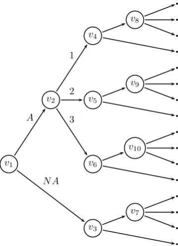
Fig. 1. Event tree for marks for two modules in a course. Marks are discretized into 3 grades, andA

andN Aindicate whether the mark is recorded or missing. The 10 situations are labelled and the 16 leaf nodes are unlabelled.

use this as our running example. The general points above translate into the following specific issues:

(1) The modules of the course are always taken in a particular order (or consistent with some partial order); there might be a requirement to achieve a threshold mark before being allowed to continue onto the next module; and certain modules might have different prerequisite modules.

(2) A student’s performance on a previous module could influence the marks on a later one.

(3) New students come in yearly cohorts. Because of any number of possible changes in any number of unobserved confounding factors the similarities in outcomes between different course histories could change for each cohort.

(4) The administrators will be interested in predicting the effect on the mark distribution by changing the program in some way, such as changing the syllabus or lecturer for a module, changing the prerequisites for a modules, or removing a module entirely. To graphically represent the different histories of a unit in the system one could use event trees (Shafer, 1996). One example of an event tree for the marks for a course with two modules is given by Figure 1.

Different situations having the same subsequent development can be viewed as a kind of conditional independence (Dawid, 1979) where the random variable describing the sub-sequent development is held to be independent of the history that led to the situation — see Studený (2005) for an overview of conditional independence structures. There are many graphical models that aim to represent conditional independence relations between the dif-ferent variables of a system. Bayesian networks (BNs) (Pearl, 2000b; Cowell et al., 1999) are currently the most prominent of these models. However, they cannot easily represent in their graphical structure the asymmetry in the potential histories of a unit. Some enhance-ments to the canonical Bayesian network have therefore been suggested in order to take this “context-specific independence” into account, for example by Boutilier et al. (1996).

Using different semantics from BNs, Smith and Anderson (2008) defined the chain event graph (CEG) as an enhancement of the event tree, where non-leaf nodes with the same probability distribution over their outgoing edges are linked by undirected edges, and where subtrees with identical probability distributions of their root-to-leaf paths are merged. Our model class is therefore based on CEGs, but extended into a more general dynamic scenario where probabilities are allowed to change with time.

In this paper we describe the dynamics of the process by a state space model incorpo-rating a switching mechanism to a neighbouring model at a given time point. The earliest example of this class, to the best of our knowledge, was studied for univariate Gaussian se-ries by Harrison and Stevens (1976) and called Multi-process Models Class II (see West and Harrison (1997) for a more recent review). Frühwirth-Schnatter (2006) reviews switching models for non-Gaussian state spaces, none of which have closed posterior forms. Here, we use a type of multi-process model which allows us to dynamically shift from one symmetry partition to another neighbouring one.

Various classes of discrete multivariate time series are of course well studied. Possibly the closest class to the one considered here are the model used in event history analysis. Event history data relates to when events of interest occur, rather than what events occur at time points of interest. Formally, an event history can be identified as amarked point process, a set{(Ts, Es) :s= 1, . . . , S}of pairs of timesTswhen eventsEsoccurred, where

the times are random variables while the events of interest are fixed beforehand, although their order might be uncertain a priori (Arjas, 1989). Two graphical models developed for event history analysis are local independence graphs (Didelez, 2008) and graphical duration graphs (Gottard, 2007). While there is an overlap between event history data and the problem outlined here, it is clear that the two address quite separate concerns. In event history analyses the number of events under consideration is typically small, with the focus of analysis being the time of events, usually allowed to occur within a continuous time domain. Here, in contrast, we wish to model a complex discrete distribution over a discrete time domain.

In order to take into account possible drifting on the tree parameters through time caused by unobserved background processes, one could follow the filtering approach of stating a transition probability P(θt | θt₋1, S), where θt represents the parameters on the tree at

form, because this speeds up computation of model goodness enormously. Thirdly, models in this class are easier to interpret when they retain their modular and conjugate forms.

Another approach, which we take here, is to set a transition function

T :P(θt₋1|xt−1, S)7→P(θt|xt−1, S) (1)

wherext−1are the observations up to timet−1. Although this approach is more restrictive

in its scope, it can be justified through various characterisations (Smith, 1979, 1992) and we show below that it can have the very attractive property of preserving the conjugate structure of each model in this class, encouraging several different authors to use such transitions.

Interventions on a graphical model are covered by the causal literature (e.g. Pearl (2000b)). Causal analysis on event trees was considered by Shafer (1996) and was defined for chain event graphs by Thwaites et al. (2010). We extend this to the dynamic model class we present here. By retaining conjugacy when learning model probability parameters, this causal extension of the model class is particularly straightforward, allowing us to utilise the model for a controlled environment.

We proceed to developing our new model, thedynamic staged tree. In Section 2 we formally define the necessary concepts. In Section 3 we develop a multi-process model for the dynamic staged tree that can be used to make one-step ahead predictions. In Section 4 we extend the multi-process model to causal analyses on the dynamic staged tree. We end in Section 5 by applying our analyses to some real educational data.

2. Concepts and definitions

2.1. Event tree

We begin the paper with some definitions; see Smith and Anderson (2008) for more details about these concepts.

LetT = (V(T), E(T))be a directed tree whereV(T)is its node set andE(T)its edge set. Let L(T) be the set of leaf nodesand S(T) = {v :v ∈V(T)\L(T)} be the set of

situations of T. Let λ(v, v′) be the path from node v ∈ S(T) to node v′ ∈ V(T) (if it exists), and letΛ(v, T) ={λ(v, v′) :v′∈L(T)}, the set of paths fromvto a leaf node. Let

X= Λ(v0, T), wherev0 is the root node ofT, so that Xis the set of root-to-leaf paths of T. Each pathX ∈Xis anatomic event, corresponding to a possible unfolding of events through time by using the partial ordering induced by the paths.

Let X(v) denote the set of children of v ∈ S(T). In an event tree(ET), each situ-ation v ∈ S(T) has an associated random variable X(v)with sample space X(v), defined conditional on having reachedv. The distribution ofX(v)is determined by theprimitive probabilitiesθ(v) ={θ(v, v′) =p(X(v) =v′) :v′∈X(v)}.

With random variables on the same path being mutually independent, the joint prob-ability of events on a path can be calculated by multiplying the appropriate primitive probabilities together. Each primitive probabilityθ(v, v′) is a colour for the directed edge

e= (v, v′), so that we letπ(e) :=θ(v, v′).

2.2. Staged trees

Starting with an event treeT, define afloretofv∈S(T)as

v

v1

v2

...

vk

−1

vk

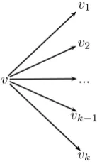
Figure 1: A floret ofv ∈S(T). This subtree represents both the random variable

X(v) and its state space _X(v).

Fig. 2. A floret of v ∈ S(T). This subtree represents both the random variableX(v) and its state spaceX(v).

whereV(F(v)) =v∪X(v)andE(F(v)) ={e∈E(T) :e= (v, v′) :v′∈X(v)}. The floret of a vertexvis thus a sub-tree consisting ofv, its children, and the edges connectingvand its children, as shown in Figure 2. This represents, as defined in section 2.1, the random variableX(v)and its sample spaceX(v).

Two situationsv, v′∈S(T)are said to be in the samestage uif and only ifX(v)and

X(v′)have the same distribution under a bijection

ψu(v, v′) :X(v)→X(v′) (3) It follows that one necessary condition forv andv′ to be in the same stage is that|X(v)|=

|X(v′)|, i.e.vandv′have the same number of children. In particular,ψu(v, v)is the identity function for any stageuthat containsv, includingu={v}.

The set of stages (orstaging) ofT is writtenU(T). It is clear thatU(T)is a partition ofS(T). The setS(T)itself can be thought of as the trivial staging.

Finally, astaged tree ST(T, U(T))is constructed from T by lettingV(ST) =V(T)

andE(ST) =Ed(ST)∪Eu(ST), where Ed(ST)andEu(ST)are constructed as follows:

• Ed(ST)is identical toE(T)except that two edges(v, v∗),(v′, v′∗)are given the same colour if and only ifv∗7→v′∗under someψu(v, v′)as defined above;

• Eu(ST): for every v, v′∈S(T), an undirected edge betweenv andv′ is drawn if and only ifX(v)andX(v′)have the same distribution.

It is easily shown (Smith and Anderson, 2008) that BNs over finite discrete random variables are an important but small subclass of staged trees.

3. Prediction with dynamic staged trees

LetT be an event tree whose topology is known and fixed in time, but with an uncertain and possibly dynamic probability distribution over its structure. Let the set of situations ofT,S(T), be denoted byS={v1, . . . , v|S|

}

.

where xt(v) = (xt(v, v′))v′∈X(v). Then at every time t we need to construct a probability

distribution over the possible values ofxtconditional on all previous observations xt−1 = (x1, . . . ,xt₋1). The marginal joint distribution P(xt) over time of the full data set can

be represented as a product of the one-step ahead predictive probabilities P(xt | xt−1).

Bayes factors associated with different models can then be expressed as a function of these quantities. It is interesting to note that this factorisation corresponds to the prequential likelihood described by Dawid (1984) used for comparing probabilistic forecasting systems. The probability distribution ofxt|xt₋1 can be written parametrically as a function of

θt, the values of θ(v)for allv∈S at time t, so that

P(xt|xt−1) =

∫

Θt

P(xt|θt,xt−1)P(θt|xt−1)dθt (4)

θtis unknown in the general case. One way to specify the distribution ofθtis to assume

the process can be described by adynamic staged tree. We define a dynamic staged tree to be an event tree where at each time pointt= 1, . . . , τ (whereτ can be finite or infinite) an independent sampling overXoccurs but with a possibly different stagingUt(T).

Ifv, v′ ∈S(T)are in the same stageuin a partitionU at timetthen we assume that

θt(v) =θt(v′),θt(u) (5)

With these assumptions, the distribution ofθtunder a stagingUtcan be written as the

product of the distribution of each stage’s parameters:

P(θt|Ut,xt−1) =

∏

u∈Ut

P(θt(u)|Ut,xt−1) (6)

Therefore equation (4) can be written as

P(xt|xt−1) =

∑

Ut∈U

∫

Θt

P(xt|θt, Ut,xt−1)P(θt|Ut,xt−1)P(Ut|xt−1)dθt (7)

= ∑

Ut∈U

∫

Θt

(

P(xt|θt, Ut,xt−1)P(Ut|xt−1)

∏

u∈Ut

P(θt(u)|Ut,xt−1)

)

dθt

(8) So to carry out a one-step ahead forecast on the system three probability distributions must be specified: the sampling distributionP(xt|xt−1,θt, Ut), the stage parameter

dis-tributionsP(θt(u)|Ut,xt−1), and the staging distributions P(Ut|xt−1). We show below how this can be achieved for each term in turn.

3.1. The sampling distributions

Under complete sampling the distribution ofX(v)for any situation v∈S is conditionally independent of any other quantity givenθ(v). In particular, this means that the distribu-tions ofX(v)andX(v′)for two situationsv, v′ ∈S,v̸=v′, are assumed to be independent conditional onθ(v), θ(v′).

This does not necessarily apply to xt(v), because the distribution of the number of

however, that for all situations v bar the root node v0 that Nt(v) equals the value of xt(v∗, v), where v∗ is the situation such that v∈X(v∗), i.e. wherev∗is the parent node of v. We discuss the setting ofNt(v0)shortly.

We can therefore writeP(xt|θt, Ut,xt−1)as

P(xt|θt, Ut,xt−1) =

∑

Nt(v0)

P(xt|Nt(v0),θt, Ut,xt−1)P(Nt(v0)|θt, Ut,xt−1) (9)

= ∑

Nt(v0)

([ ∏

v∈S

P(xt(v)|θt(v), xt(v∗, v))

]

P(Nt(v0)|θt, Ut,xt−1)

)

(10)

= ∑

Nt(v0)

   ∏

v∈S

I{∑xt(v,v′)=xt(v∗,v)}

∏

v′_∈X(v)

θt(v, v′)xt(v,v′)



P(Nt(v0)|θt, Ut,xt−1)

 

(11) where IA is the indicator variable for an event A and xt(v∗, v0) is understood to mean Nt(v0).

The modelling of the distribution of Nt(v0)depends on the details of the system under

consideration. One common scenario is when Nt(v0) is believed to be independent of all

other system parameters apart from, at most, values ofNs(v0)fors < t. One approach in

this case is to modelNt(v0)as a Poisson variable with parameterλ, whereλcan either be

constant or itself given a conjugate prior of Gamma(αλ, βλ)at time 1. WhenNt(v0)is known, equation (11) becomes

P(xt|θt, Ut,xt−1) =

∏

v∈S

 _I{∑_x

t(v,v′)=xt(v∗,v)}

∏

v∗_∈X(v)

θt(v, v′)xt(v,v′)



 (12)

wherext(v∗, v0)should again be read asNt(v0).

3.2. The stage parameter distributions

As with every aspect of the model, the specification of the probability distribution over the floret parameters for each possible stage should be tailored to the scenario at hand. In many cases, however, it is possible to characterise the distribution from some common qualitative modelling assumptions.

Consider first the trivial stagingUt=S. It is shown in Freeman and Smith (2009) that if it is assumed that the relative rates of the root-to-leaf paths are independent, then the additional assumption of mutual independence of the floret distributions implies that each non-trivial floret’s distribution must be Dirichlet. Therefore, denoting its set of hyperpa-rameters asαt(v) = (αt(v, v′))v′∈X(v), the density ofθt(v)| Ut =S,xt−1 for a non-trivial

floretv∈S is

fθt(v)(θt(v)|Ut=S,xt−1) = Γ

  ∑

v′∈X(v)

αt(v, v′)

  ∏

v′∈X(v)

θt(v, v′)αt(v,v′)−1 Γ(αt(v, v′))

(13)

Now consider a staging U that is not a trivial partition of S. In Freeman and Smith (2009) we show that requiringmargin equivalencyto hold for its stagesu∈U charac-terises the prior on the floret distributions. A stageuhas margin equivalency when

P(X(u)|θ, U) =P(X(u)|θ, S). (14)

whereX(u)is the random variable with sample space∪_v′_∈vu{v′∪ {

∪

v∈uψ(vu, v)(v′)}}, i.e.

the edge equivalence classes under a stage. This property is analogous to that of parameter modularity for Bayesian networks (Heckerman, 1999). With the distribution for florets in

Sgiven above, this implies that the prior probability ofθt(u)|Ut=U,xt−1 _{has a Dirichlet}

distribution too, with hyperparameters that are sums of the corresponding hyperparameters underS of the constituent florets:

fθt(u)(θt(u)|Ut=U,xt−1) = Γ



 ∑

v′∈X(vu) ¯ αt(u, v′)



 ∏

v′∈X(vu)

θt(u, v′)α¯t(u,v′)−1

Γ( ¯αt(u, v′)) (15)

wherevu is any situation inu,θt(u, v′)are the elements of the vectorθt(u)andα¯t(u, v′) =

∑

v:v∈uαt(v, ψu(vu, v)(v′)). Informally, equation (15) says that the hyperparameter vector

for all of the floret distributions of the situations in stage u is equal to the sum of the hyperparameter vectors of the floret distributions underS.

With margin equivalency and independence between the floret distributions under S, the floret distributions under different stagings for stages composed of the same situations will always be the same. Therefore the probability distributions for a stage’s parameters (13) and (15) depend only the composition of the stage and not on the rest of the staging. This property is useful since it allows us to discuss the characteristics of stage clusters of variable groups without reference to the partition in which they appear. This makes individual models much simpler to explain. It also reduces the computational complexity in calculating (13) and (15) because they will not be dependent on staging.

As everyθt(u)is conditionally independent of all other quantities givenαt(u) = (αt(v))v∈u,

settingP(θt|Ut,xt−1)only requires the setting ofαt(v)for eachv ∈S for everyt. This

task can be simplified further by assuming

ft+1,v(θ) =T(ft,v∗ (θ)) (16)

for some functionT for allt >1, whereft,v(θ)is the density ofθt(v)|xt−1, Ut=Sas given

in equation (13), and f_t,v∗ (θ)is the density of θt(v) | xt, Ut =S, so that for every v ∈ S

onlyα1(v)needs to be set.

The simplest choice ofT is the identity functional, so thatft+1,v(θ) =ft,v∗ (θ)fort >1.

With ft,v(θ) as given in equation (13) and P(xt(v) | θt(v)) ∝∏_v′_∈X(v)θt(v, v′)

xt(v,v′) as

given by equation (11), Bayes’ theorem requires

f_θ∗

t(v)(θt(v)|x t_{) = Γ}

  ∑

v′∈X(v)

α∗_t(v, v′)

  ∏

v′∈X(v)

θt(v, v′)α∗_t(v,v′)−1

Γ(α∗_t(v, v′)) (17)

whereα∗t(v, v′) =αt(v, v′) +xt(v, v′), and so

As equation (18) is true for allt >1, αt(v)can be written as a function of onlyα1(v)and xt−1_(v),

αt(v) =α1(v) + t−1

∑

τ=1

xτ(v) (19)

for allv∈S.

LettingT be the identity functional reflects a modelling assumption that the underlying probabilities associated with each stage do not evolve from year to year for a given staged tree. Sometimes this will be too strong an assumption to make. In this case, a weaker set of assumptions are needed which will represent the fact that there is an “information drift” between the time points. This will also guard against spurious jumps in the model probabilities from expected model drift.

One way to characteriseT to meet this need is provided by thepower steady model

(Smith, 1979, 1981, 1992). It was shown by Smith (1979) that if, loosely speaking, it is assumed that the Bayes decision under a step loss function would stay the same over time if no more information was gathered about the system but that the expected loss of the decision increases due to increasing uncertainty, then it is required that

ft+1,v(θ)∝(ft,v∗ (θ))

k ₍₂₀₎

for some0< k≤1.

This transition function has a number of appealing properties. Firstly, when applied to the joint distributionP(θt|Ut,xt−1)of theθunder any stagingUt, the floret independence

structure is kept intact.

Secondly, it can be shown that use of the steady model guards against misspecified priors, making predictions more robust. Let the local de Robertis measureDRA be

defined as follows (Smith and Daneshkhah, 2010):

dL_A(f, g) = sup

θ,ϕ∈A

{(logf(θ)−logg(θ))−(logf(ϕ)−logg(ϕ))} (21)

for any A ∈ Θ. Smith and Daneshkhah (2010) show that the local de Robertis mea-sure is a separation meamea-sure where its separations do not change under Bayesian updating (Smith and Daneshkhah, 2010). It therefore represents artifacts of the model that cannot be changed by observation. It can easily be shown that, wheref∗∝fk _{and similarly forg,} dL_A(f∗, g∗) =k(dL_A(f, g)), (22) Thus using the steady model brings distributions closer together when0 < k≤1. In this sense steady models tend to be robust against initial prior misspecification, if we seef as the prior used in the analysis and g as the “true” prior. See Smith and Rigat (2008) for further details.

A similar result can be shown for Kullback-Leibler (KL) distances (Kullback and Leibler, 1951): recall that for two densitiesf andg the KL distance is given by

dKL(f;g) =

∫

(logf(θ)−logg(θ))g(θ)dθ

and that the entropyH of a density is given by

H(f) =−

∫

Letf1, f2be any two densities such thatH(f1) =H(f2). Then

dKL(pt+1;f1)−dKL(pt+1;f2) =k(dKL(pt;f1)−dKL(pt;f2)) (23)

whereptis the density of the stage parameters at timet, both after observingxt, so that pt+1∝(pt)k. Equation (23) says that the distance between the density of the stage

param-eters under any staging and two arbitrary densities with the same entropy decreases by a fixed proportion at each time step, again indicating a robustness to prior mis-specification. Thirdly, withα∗_t(v) =αt(v)+xt(v), equation (20) implies thatθt+1(v)is still distributed

Dirichlet ifθt(v)is Dirichlet but with the hyperparameters of the distribution now given by the values

αt+1(v, v′) =kαt(v, v′) +kxt(v, v′)−k+ 1 (24)

Solving this recurrence relation for a constantk yields

αt(v, v′) =kt−1(α1(v, v′)−1) + t−1

∑

τ=1

kt−τxτ(v, v′) + 1 (25)

which heuristically can be seen as weighting recent observations more heavily for the setting of the latest prior.

Each situation can have its own k, k(v), and it might be desired that this k(v) be different for differentt, for example when an external intervention in the system occurs.

We note that the use of the power steady model has a long history with Dirichlet distributions (e.g. in Smith (1979); Queen et al. (1994); Cowell et al. (1999)) and more generally (e.g. Ibrahim and Chen (2000); Rigat and Smith (2009)), and has also been used in Bayesian forecasting under the alternative name of exponential forgetting (Raftery et al., 2010). Here we use the power steady model as a justifiable and conjugate method for making inference about tree models whose floret probabilities evolve.

3.3. The staging distributions

We have allowed for drift over time in the values of probabilities associated with the con-ditional independence structure implicit in a staged tree model. However, we also want to allow for the possibility that the tree stagings themselves — and not just their parameters — evolve in time. It is unfeasible and usually unnecessary to model all possible changes of this partition space; in most applications it is appropriate to assume that changes in stage structure will be small in number and occur locally.

We therefore propose a dynamic model for the staged trees analogous to the Class 2 Multi-process Models used for dynamic linear models (DLMs) (Harrison and Stevens, 1976; West and Harrison, 1997). This was developed for the case where “no single [model] adequately describes what might happen to the process in the next time interval” (West and Harrison, 1997). We describe the C2MPM here as it applies to the staged tree setting. Let U be the set of all possible stagings of T, and for each U ∈ U and t > 1 let

πt(U) = P(Ut =U | xt−1). There is obviously a large class of possible specifications for πt(U), but we note the three “practically important possibilities” mentioned by (West and

Harrison, 1997):

(1) Fixed model selection probabilities, such that

Here, one needs to only specify one prior over U. This prior remains fixed through time and isn’t changed by observations.

(2) First-order Markov probabilities, where fixed transition probabilities between the models

π(U |U′) =P(Ut=U |Ut₋1=U′) (27)

are specified a priori, so that

πt(U) =

∑

U′∈U

π(U |U′)P(Ut−1=U′|xt−1) (28)

Some initial prior distribution over the staged tree space, π1(C), would need to be

set.

(3) Higher-order Markov probabilities, where the probabilities of the stagings at timet

additionally depend on the stagings att−2,t−3, etc.

While the first possible modelling strategy, of fixed staging probabilities, is much the simpler one (and the option used by West and Harrison for exposition), the second and third strategies are often going to be more accurate reflections of experts’ beliefs. We show here how to implement first-order Markov transitions between stagings.

A common assumption will be thatπ(U |U′)is larger the “closer” U is toU′ in some sense, so that the underlying process is unlikely to change too much over a short period of time. Ifπ(U |U′) = 0 for someU ∈U, this has the advantage of reducing the number of terms in equation (28).

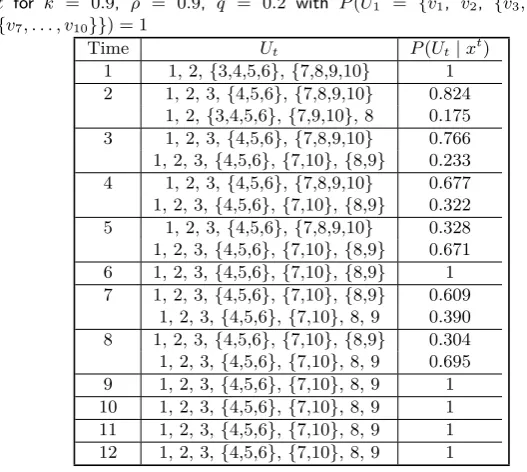
We therefore require a metric onU and then letπ(U |U′)be a function of this metric. Any intuitive metric on general sets of partitions can be used, e.g. that of Meilă (2007). A simple metric that we use here can be derived from the Hasse diagram of the lattice of partitions ofS under the relation “finer than” (see Stanley (1997) for a detailed overview of such lattice terminology). The Hasse diagram for|S|= 4is shown in Figure 3.

The length of the shortest path between two partitions on the Hasse diagram is a metric on the partition space ofS, and we call itℓhere. A distance ofℓ= 1represents the division of a stage or the merging of two stages. One possible way to set π(U |U′) based on this metric is

π(U |U′) =

    

ρ ifU =U′

|Bϵ(U′)|−1(1−ρ) if0< ℓ(U, U′)≤ϵ,

0 otherwise

(29)

whereBϵ(U′) ={U ∈U :ℓ(U, U′)≤ϵ, U ̸=U′, U ∈U}is an ϵ-ball of stagings aroundU′

under theℓmetric. This represents a belief that the underlying symmetry process changes only locally and slowly. If more radical changes in the symmetry process are taking place due to external intervention in the system then the methodology in Section 4.1 can be deployed.

The other term in (27), P(Ut₋1 = U′ | xt−1), can be calculated for eachUt−1 using

Bayes’ theorem:

P(Ut₋1=U′|xt−1)∝P(xt₋1|Ut₋1=U′)P(Ut₋1=U′|xt−2) (30) = P(xt−1|Ut−1=U

′_)P(U

t−1=U′|xt−2)

∑

U′_∈UP(xt₋1|Ut₋1=U′)P(Ut₋1=U′ |xt−2)

{1,2,3,4}

{1,4},{2,3} 1,{2,3,4} {1,2,4},3 {1,3},{2,4} {1,2,3},4 {1,3,4},2 {1,2},{3,4}

1,{2,3},4 {1,4},2,3 1,{2,4},3 {1,3},2,4 {1,2},3,4 1,2,{3,4}

1,2,3,4

Fig. 3. The Hasse diagram of the lattice of partitions ofS when|S|= 4

TheP(Ut−1=U′ |xt−2)terms on the right-hand side of (31) will be already be available

at time t−1. The term P(xt−1 | Ut−1 = U′), meanwhile, can be calculated as follows,

using equations (11) and (15) at timet−1:

P(xt−1|Ut−1=U′) =

∫

Θt−1

P(xt−1|θt−1, Ut−1=U′)P(θt−1|Ut−1=U′)dθt−1 (32)

∝

∫

Θt₋1

∏

u∈U′

 Γ

  ∑

v′∈X(vu) ¯

αt−1(u, v′)



 ∏

v′∈X(vu)

θt₋1(u, v′)α¯

∗

t−1(u,v′)−1

Γ( ¯αt−1(u, v′))

 dθt−1

(33)

= ∏

u_∈U′

 Γ

(∑

v′∈X(vu)αt¯ −1(u, v′)

)

Γ(∑_v′_∈X(vu)α¯∗t−1(u, v′)

) ∏

v′∈X(vu)

Γ( ¯α∗_t−1(u, v′)) Γ( ¯αt₋1(u, v′))



 (34)

wherevu is any situation inu,α¯_t∗₋₁(u, v′) = ¯xt₋1(u, v′) + ¯αt₋1(u, v′), wherext¯₋1(u, v′) =

∑

v:v_∈uxt−1(v, ψu(vu, v)(v′))andαt¯₋1 is as defined in equation (15).

The number of terms in (28) can be reduced further by setting the values ofP(Ut₋1= U′ | xt−1_{) below a threshold q as zero and normalising the remaining probabilities to}

ensure they still sum to 1. A similar approach advocated by Madigan and Raftery (1994) as “Occam’s window” is to discard modelsU′ that are not in the set

Ut∗=

{

Ut∈U : P(Ut|x t₎

maxUP(U |xt) ≤ q

}

(35)

3.4. One-step-ahead prediction

Equation (7) can now be written, using the foregoing, as

P(xt|xt−1) =

∑

Ut∈U

∫

Θt

  ∑

Ut−1∈U

π(Ut|Ut₋1)P(Ut−1|xt−1)

 

  ∑

Nt(v0)

P(Nt(v0)|θt, Ut,xt−1)

· ∏

u_∈Ut IA



Γ( ∑ v′∈X(vu)

¯ αt(u, v′)

)

· ∏

v′∈X(vu)

θt(u, v′)α¯t(u,v

′_)+¯x

t(u,v′)−1 Γ( ¯αt(u, v′))

 

 dθt

(36) whereAis the event ∀v∈u\v0,

∑

v′xt(v, v′) =xt(v∗, v). If it is assumed that the

distri-bution ofNt(v0)depends only onxt−1then (36) can be further simplified to the closed-form

solution

P(xt|xt−1) =

∑

U_t∈U

(   ∑

Ut−1∈U

π(Ut|Ut−1)P(Ut−1|xt−1)

 

  ∑

Nt(v0)

P(Nt(v0)|xt−1)

· ∏

u_∈Ut IA

 Γ

(∑

v′_∈X(vu)αt(u, v¯ ′₎)

Γ(∑_v′_∈X(vu)α¯ ∗ t(u, v′)

) ∏

v′∈X(vu)

Γ( ¯α∗_t(u, v′)) Γ( ¯αt(u, v′))

 

 

)

(37) IfNt(v0)is always known, then (37) can be simplified further to become

P(xt|xt−1) =

∑

Ut∈U

(   ∑

Ut−1∈U

π(Ut|Ut₋1)P(Ut₋1|xt−1)

 

· ∏

u∈Ut IA

 Γ

(∑

v′∈X(vu)α¯t(u, v ′₎)

Γ(∑_v′_∈X(vu)α¯ ∗ t(u, v′)

) ∏

v′∈X(vu)

Γ( ¯α∗_t(u, v′)) Γ( ¯αt(u, v′))

 

)

(38)

4. Causal intervention

With any forecasting system there is also an attendant need to consider the effects of external intervention in the system, including by the forecasters themselves (West and Harrison, 1989). This ensures that all relevant information is taken into account, increasing the accuracy of future forecasts.

We believe that tree-based graphical models are very useful in general for carrying causal analysis. Due to the multiple representations of each variable in the graph — one for each possible path-history on parent variables — much more refined interventions in the system can be represented (Shafer, 1996). How causal hypotheses can be represented within the framework of static CEGs has been investigated by Thwaites and Smith (2006) and Thwaites et al. (2010).

We now show how causal analysis affects the one-step ahead forecast on a dynamic staged tree given by equations (36), (37), and (38) for two different types of intervention: one on the possible stagings on a treeT and one on the structure of the treeT itself.

4.1. Intervention on the staging distribution

Suppose that at time t some situations will be moved into their own stage u, leaving all other stages intact. For example, in our educational example, the exams for the second module might be tailored so that performance in the first module is no longer a predictor in how well students should perform in it. The one-step ahead forecasts can then be modified in the following way to reflect this intervention.

Recall that π_t∗₋₁(U) =P(Ut−1=U |xt−1). Let π†t(U) = P(Ut=U |xt−1, It), where It is the intervention described above. Then one approach to modelling the intervention is

to setπ_t†(U) =π∗_t−1(U)for each U ∈U such thatu∈U, and set π_t†(U†) =π∗_t−1(U)and

π_t†(U) = 0 for U ∈U such that u ̸∈ U, whereU† is the same as U except that u ∈U†

and other stages that contained situationsv∈uare reduced accordingly. The effect of this approach is to transfer the probability massed on the stagings where u ̸∈ U to stagings whereu∈U .

One issue that now arises is how the distribution ofθt|Ut is affected. In the absence

of further information, a good default is to use the steady model as in the idle system but with a lower value for the steady parameter k. This indicates that past data might not be as useful in helping to make predictions in this situation as under the idle system. We note that this is analogous to setting a higher variance on evolution parameters in dynamic linear models when forecasting after interventions is required for that model class (Section 1.2.2 of West and Harrison (1997)).

4.2. Intervention onT

Recalling the event tree pictured in Figure 1, consider the case where at timet the course directors decide to eliminate the first module on the tree from course. This means that the marks that students would have got for this module are unknown from that time onwards, and therefore all of the data at timet for this module will be concentrated on the second (“NA”) edge of thev1 floret.

This type of intervention is analogous to thedooperator introduced for CBNs by (Pearl, 2000a), where a random variable is forced to take a particular value with probability 1. The difference with CBNs is that staged trees allow a richer set of interventions on their structure, including letting an intervention take place at specific time and situations, and not merely changing the value of a variable under all circumstances.

occurs.

Without loss of generality, say that at timetan interventionIt(v, v′)at situationv∈S

occurs so thatθt(v, v′)is equal to 1 for a specificv′ ∈X(v)and to 0 for all otherv∗∈X(v). By the definition of the event tree, along with the causal assumptions, all other floret distributions are technically unchanged. However, notice that the probability of reaching any node in anyΛ(v∗, T), the sub-tree withv∗ as the root node, is zero. It follows that the treeT is equivalent to the reduced treeT′ where allΛ(v∗, T)are deleted and only the edge

(v, v′)remains in the floretF(v), and so the process can henceforth be considered to take place on this reduced treeT′.

The one-step ahead forecasts can now be calculated as before with a few modifications due the set of situationsSchanging; call this new setS†. Firstly, the distribution overU†, the new set of possible stagings, must be set. There are several possible choices here. In the absence of any other information, a good default is to let

P(Ut=U†|xt−1, It(v, v′)) =P(Ut₋1=U |xt−1), (39)

where U† is the staging formed from U by replacing each stage u∈ U with a new stage

u† := u\ {v†}v†∈S\S†, and by splitting the stage u† ∈ U† that contains the intervention

nodev intou†\v andv.

Secondly, the distributions of the stage parametersθt(u)for anyuneed to be

reconsid-ered. Under the causal assumptions considered here, interventions have only local effects, so a sensible default model is to letfθt(u)(θt(u) |Ut =U,x

t−1_{, I}

t(v, v′))be calculated as

before, i.e. as given in Equation (15).

Assuming that all of the other system characteristics, e.g. the steady model and the multinomial sampling, are intact post-intervention, the one-step ahead forecast (37) is ad-justed to become

P(xt|xt−1, It(v, v′)) =

∑

U_t†∈U†

(   ∑

Ut−1∈U

π†(Ut†|Ut−1)P(Ut−1|xt−1)

 

  ∑

Nt(v0)

P(Nt(v0)|xt−1)

· ∏

u∈U_t† IA

 Γ

(∑

v′∈X(vu)α¯t(u, v′)

)

Γ(∑_v′_∈X(vu)α¯∗t(u, v′)

) ∏

v′_∈X(vu)

Γ( ¯α∗t(u, v′)) Γ( ¯αt(u, v′))

 

 

)

(40)

whereπ†(U_t†|Ut−1) =π(Ut|Ut−1)by the argument above.

5. A simple educational example

In this section we illustrate how to carry out one-step ahead predictions with dynamic staged trees using 12 years’ worth of exam marks for two first-year undergraduate modules. The underlying event tree used was that shown in Figure 1.

We made the following assumptions:

(1) Nt(v0)was known for all values oft

(2) The distribution over the root-to-leaf paths at timet= 1underU1=Swas Dirichlet

Table 1. All possible stagings and their posterior probabilities at each time

t for k = 0.9, ρ = 0.9, q = 0.2 with P(U1 = {v1, v2, {v3, . . . , v6},

{v7, . . . , v10}}) = 1

Time Ut P(Ut|xt)

1 1, 2, {3,4,5,6}, {7,8,9,10} 1 2 1, 2, 3, {4,5,6}, {7,8,9,10} 0.824

1, 2, {3,4,5,6}, {7,9,10}, 8 0.175 3 1, 2, 3, {4,5,6}, {7,8,9,10} 0.766 1, 2, 3, {4,5,6}, {7,10}, {8,9} 0.233 4 1, 2, 3, {4,5,6}, {7,8,9,10} 0.677 1, 2, 3, {4,5,6}, {7,10}, {8,9} 0.322 5 1, 2, 3, {4,5,6}, {7,8,9,10} 0.328 1, 2, 3, {4,5,6}, {7,10}, {8,9} 0.671 6 1, 2, 3, {4,5,6}, {7,10}, {8,9} 1 7 1, 2, 3, {4,5,6}, {7,10}, {8,9} 0.609

1, 2, 3, {4,5,6}, {7,10}, 8, 9 0.390 8 1, 2, 3, {4,5,6}, {7,10}, {8,9} 0.304 1, 2, 3, {4,5,6}, {7,10}, 8, 9 0.695 9 1, 2, 3, {4,5,6}, {7,10}, 8, 9 1 10 1, 2, 3, {4,5,6}, {7,10}, 8, 9 1 11 1, 2, 3, {4,5,6}, {7,10}, 8, 9 1 12 1, 2, 3, {4,5,6}, {7,10}, 8, 9 1

(3) For the transitions between stagings we used theℓmetric withϵ= 1, i.e. only transi-tions between models with local changes were considered possible.

We present here the posterior probabilities P(Ut |xt) for the stagings after t = 1 for

each timetfor different hyperparameter values, when analysed with and without an external intervention.

In a full analysis this application could be run over a distribution of the hyperparameters

k(the steady model parameter),ρ(the probability of the underlying model not changing) and q (the Occam’s window threshold), perhaps after taking account of an elicited prior over their possible values. However, to illustrate the efficacy of our methods rather than learn these hyperparameters it is better to hold them fixed so that we can better focus on the impact of various structured assumptions we learn about.

5.1. Analysis of the series without intervention

In Table 5.1 we present P(Ut | xt) for t = 1. . .12 for the model where U1 = {v1, v2,

{v3, . . . , v6},{v7, . . . , v10}}with probability 1 andk= 0.9,ρ= 0.9andq= 0.2. The latter

two parameter values ensure that few new models will be kept in the analysis, as the high value ofρ gives a low prior probability on transitions between stagings and this value of

qmakes the Occam’s window set of equation (35) small. This speeds up the computation of the forecasts at the expense of possibly worse predictions through fewer stagings being included in the model averaging.

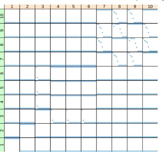
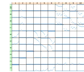
An alternative way of presenting this information is to plot how P(vi, vj ∈ u), the

probability that situationsvi, vj are in the same stage, changes for increasing values of t.

● ● ● ● ● ● ● ● ● ● ● ●1 1 ● ● ● ● ● ● ● ● ● ● ● ● 2 1 ● ● ● ● ● ● ● ● ● ● ● ● 3 1 ● ● ● ● ● ● ● ● ● ● ● ● 4 1 ● ● ● ● ● ● ● ● ● ● ● ● 5 1 ● ● ● ● ● ● ● ● ● ● ● ● 6 1 ● ● ● ● ● ● ● ● ● ● ● ● 7 1 ● ● ● ● ● ● ● ● ● ● ● ● 8 1 ● ● ● ● ● ● ● ● ● ● ● ● 9 1 ● ● ● ● ● ● ● ● ● ● ● ● 10 1 ● ● ● ● ● ● ● ● ● ● ● ● 1 2

● ● ● ● ● ● ● ● ● ● ● ●2

2 ● ● ● ● ● ● ● ● ● ● ● ● 3 2 ● ● ● ● ● ● ● ● ● ● ● ● 4 2 ● ● ● ● ● ● ● ● ● ● ● ● 5 2 ● ● ● ● ● ● ● ● ● ● ● ● 6 2 ● ● ● ● ● ● ● ● ● ● ● ● 7 2 ● ● ● ● ● ● ● ● ● ● ● ● 8 2 ● ● ● ● ● ● ● ● ● ● ● ● 9 2 ● ● ● ● ● ● ● ● ● ● ● ● 10 2 ● ● ● ● ● ● ● ● ● ● ● ● 1 3 ● ● ● ● ● ● ● ● ● ● ● ● 2 3

● ● ● ● ● ● ● ● ● ● ● ●3

3 ● ● ● ● ● ● ● ● ● ● ● ● 4 3 ● ● ● ● ● ● ● ● ● ● ● ● 5 3 ● ● ● ● ● ● ● ● ● ● ● ● 6 3 ● ● ● ● ● ● ● ● ● ● ● ● 7 3 ● ● ● ● ● ● ● ● ● ● ● ● 8 3 ● ● ● ● ● ● ● ● ● ● ● ● 9 3 ● ● ● ● ● ● ● ● ● ● ● ● 10 3 ● ● ● ● ● ● ● ● ● ● ● ● 1 4 ● ● ● ● ● ● ● ● ● ● ● ● 2 4 ● ● ● ● ● ● ● ● ● ● ● ● 3 4

● ● ● ● ● ● ● ● ● ● ● ●4

4

● ● ● ● ● ● ● ● ● ● ● ●5

4

● ● ● ● ● ● ● ● ● ● ● ●6

4 ● ● ● ● ● ● ● ● ● ● ● ● 7 4 ● ● ● ● ● ● ● ● ● ● ● ● 8 4 ● ● ● ● ● ● ● ● ● ● ● ● 9 4 ● ● ● ● ● ● ● ● ● ● ● ● 10 4 ● ● ● ● ● ● ● ● ● ● ● ● 1 5 ● ● ● ● ● ● ● ● ● ● ● ● 2 5 ● ● ● ● ● ● ● ● ● ● ● ● 3 5

● ● ● ● ● ● ● ● ● ● ● ●4

5

● ● ● ● ● ● ● ● ● ● ● ●5

5

● ● ● ● ● ● ● ● ● ● ● ●6

5 ● ● ● ● ● ● ● ● ● ● ● ● 7 5 ● ● ● ● ● ● ● ● ● ● ● ● 8 5 ● ● ● ● ● ● ● ● ● ● ● ● 9 5 ● ● ● ● ● ● ● ● ● ● ● ● 10 5 ● ● ● ● ● ● ● ● ● ● ● ● 1 6 ● ● ● ● ● ● ● ● ● ● ● ● 2 6 ● ● ● ● ● ● ● ● ● ● ● ● 3 6

● ● ● ● ● ● ● ● ● ● ● ●4

6

● ● ● ● ● ● ● ● ● ● ● ●5

6

● ● ● ● ● ● ● ● ● ● ● ●6

6 ● ● ● ● ● ● ● ● ● ● ● ● 7 6 ● ● ● ● ● ● ● ● ● ● ● ● 8 6 ● ● ● ● ● ● ● ● ● ● ● ● 9 6 ● ● ● ● ● ● ● ● ● ● ● ● 10 6 ● ● ● ● ● ● ● ● ● ● ● ● 1 7 ● ● ● ● ● ● ● ● ● ● ● ● 2 7 ● ● ● ● ● ● ● ● ● ● ● ● 3 7 ● ● ● ● ● ● ● ● ● ● ● ● 4 7 ● ● ● ● ● ● ● ● ● ● ● ● 5 7 ● ● ● ● ● ● ● ● ● ● ● ● 6 7

● ● ● ● ● ● ● ● ● ● ● ●7

7 ● ● ● ● ● ● ● ● ● ● ● ● 8 7 ● ● ● ● ● ● ● ● ● ● ● ● 9 7

● ● ● ● ● ● ● ● ● ● ● ●10

7 ● ● ● ● ● ● ● ● ● ● ● ● 1 8 ● ● ● ● ● ● ● ● ● ● ● ● 2 8 ● ● ● ● ● ● ● ● ● ● ● ● 3 8 ● ● ● ● ● ● ● ● ● ● ● ● 4 8 ● ● ● ● ● ● ● ● ● ● ● ● 5 8 ● ● ● ● ● ● ● ● ● ● ● ● 6 8 ● ● ● ● ● ● ● ● ● ● ● ● 7 8

● ● ● ● ● ● ● ● ● ● ● ●8

8 ● ● ● ● ● ● ● ● ● ● ● ● 9 8 ● ● ● ● ● ● ● ● ● ● ● ● 10 8 ● ● ● ● ● ● ● ● ● ● ● ● 1 9 ● ● ● ● ● ● ● ● ● ● ● ● 2 9 ● ● ● ● ● ● ● ● ● ● ● ● 3 9 ● ● ● ● ● ● ● ● ● ● ● ● 4 9 ● ● ● ● ● ● ● ● ● ● ● ● 5 9 ● ● ● ● ● ● ● ● ● ● ● ● 6 9 ● ● ● ● ● ● ● ● ● ● ● ● 7 9 ● ● ● ● ● ● ● ● ● ● ● ● 8 9

● ● ● ● ● ● ● ● ● ● ● ●9

9 ● ● ● ● ● ● ● ● ● ● ● ● 10 9 ● ● ● ● ● ● ● ● ● ● ● ● 1 10 ● ● ● ● ● ● ● ● ● ● ● ● 2 10 ● ● ● ● ● ● ● ● ● ● ● ● 3 10 ● ● ● ● ● ● ● ● ● ● ● ● 4 10 ● ● ● ● ● ● ● ● ● ● ● ● 5 10 ● ● ● ● ● ● ● ● ● ● ● ● 6 10 ● ● ● ● ● ● ● ● ● ● ● ● 7 10 ● ●● ● ● ● ● ● ● ● ● ● 8 10 ● ● ● ● ● ● ● ● ● ● ● ● 9 10 ● ● ● ● ● ● ● ● ● ● ● ● 10 10

Fig. 4. Plots of probabilities that each pair of situations are in the same stage for different values oft, for the case whenk= 0.9,ρ= 0.9,q= 0.2withP(U1={v1,v2,{v3, . . . , v6},{v7, . . . , v10}}) = 1, using the values in Table 5.1

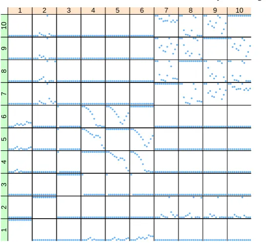
To illustrate how the level of detail in the staging distribution changes as a function the hyperparameters, we carried out the analysis again with radically different values: we set k = 0.5 (so that floret distributions are flattened more quickly and therefore past observations more heavily discounted),ρ= 0.25(so that the probability of moving between stagings is more likely), andq= 0.05(so that stagings with poorer Bayes factors relative to the most likely are kept in the analysis) withP(U1={v1,v2,{v3, . . . , v6},{v7, . . . , v10}}) = 1still assumed for consistency. The resulting matrix plot of probabilities of situations being in the same stage against time is as shown in Figure 5.

It can be seen from the latter figure that the analysis with the new hyperparameter values gives much the same qualitative description of the system as the more conservative hyperparameters at greater computational expense, with the pay-off of greater detail.

Some interesting characteristics of the system can be discerned from this initial ex-ploratory analysis of this system. With regard to the situations concerning whether marks are available for a module or not,θ(v3)— the probability distribution for the second

mod-ule’s marks being available given that the mark in the first module is itself missing — does not appear to be related to the others at any time point. Until t = 7, v4, v5 and v6, the

situations representing the probability of marks being missing in the second module after gaining a high, medium or low mark respectively in the first module, had high but falling probabilities of being in the same stage, implying that independence of the second module’s marks being missing from skill in the first module kept decreasing from a high point. At

● ● ● ● ● ● ● ● ● ● ● ●1 1 ● ● ● ● ● ● ● ● ● ● ● ● 2 1 ● ● ● ● ● ● ● ● ● ● ● ● 3 1 ● ● ●●● ● ●● ● ● ● ● 4 1 ● ● ●●● ● ● ●●● ● ● 5 1 ● ● ●●● ●● ● ● ● ● ● 6 1 ● ● ● ● ● ● ● ● ● ● ● ● 7 1 ● ● ● ● ● ● ● ● ● ● ● ● 8 1 ● ● ● ● ● ● ● ● ● ● ● ● 9 1 ● ● ● ● ● ● ● ● ● ● ● ● 10 1 ● ● ● ● ● ● ● ● ● ● ● ● 1 2

● ● ● ● ● ● ● ● ● ● ● ●2

2 ● ● ● ● ● ● ● ● ● ● ● ● 3 2 ● ● ● ● ● ● ● ● ● ● ● ● 4 2 ● ● ● ● ● ● ● ● ● ● ● ● 5 2 ● ● ● ● ● ● ● ● ● ● ● ● 6 2 ● ● ● ● ● ● ● ● ● ● ● ● 7 2 ● ● ●●●● ● ● ● ● ● ● 8 2 ● ● ● ● ●● ● ● ● ● ● ● 9 2 ● ● ● ● ● ● ● ● ● ● ● ● 10 2 ● ● ● ● ● ● ● ● ● ● ● ● 1 3 ● ● ● ● ● ● ● ● ● ● ● ● 2 3

● ● ● ● ● ● ● ● ● ● ● ●3

3 ● ● ● ● ● ● ● ● ● ● ● ● 4 3 ● ● ● ● ● ● ● ● ● ● ● ● 5 3 ● ● ● ● ● ● ● ● ● ● ● ● 6 3 ● ● ● ● ● ● ● ● ● ● ● ● 7 3 ● ● ● ● ● ● ● ● ● ● ● ● 8 3 ● ● ● ● ● ● ● ● ● ● ● ● 9 3 ● ● ● ● ● ● ● ● ● ● ● ● 10 3 ● ● ● ●● ● ●●● ● ● ● 1 4 ● ● ● ● ● ● ● ● ● ● ● ● 2 4 ● ● ● ● ● ● ● ● ● ● ● ● 3 4

● ● ● ● ● ● ● ● ● ● ● ●4

4 ● ●● ● ● ● ● ● ● ● ● ● 5 4 ● ● ● ● ● ● ● ● ● ● ● ● 6 4 ● ● ● ● ● ● ● ● ● ● ● ● 7 4 ● ● ● ● ● ● ● ● ● ● ● ● 8 4 ● ● ● ● ● ● ● ● ● ● ● ● 9 4 ● ● ● ● ● ● ● ● ● ● ● ● 10 4 ● ● ●●●●● ●●● ● ● 1 5 ● ● ● ● ● ● ● ● ● ● ● ● 2 5 ● ● ● ● ● ● ● ● ● ● ● ● 3 5 ● ●● ● ● ● ● ● ● ● ● ● 4 5

● ● ● ● ● ● ● ● ● ● ● ●5

5 ● ●● ● ● ● ● ● ●● ● ● 6 5 ● ● ● ● ● ● ● ● ● ● ● ● 7 5 ● ● ● ● ● ● ● ● ● ● ● ● 8 5 ● ● ● ● ● ● ● ● ● ● ● ● 9 5 ● ● ● ● ● ● ● ● ● ● ● ● 10 5 ● ● ●● ●●● ● ● ● ● ● 1 6 ● ● ● ● ● ● ● ● ● ● ● ● 2 6 ● ● ● ● ● ● ● ● ● ● ● ● 3 6 ● ● ● ● ● ● ● ● ● ● ● ● 4 6 ● ● ● ● ● ● ● ● ●● ● ● 5 6

● ● ● ● ● ● ● ● ● ● ● ●6

6 ● ● ● ● ● ● ● ● ● ● ● ● 7 6 ● ● ● ● ● ● ● ● ● ● ● ● 8 6 ● ● ● ● ● ● ● ● ● ● ● ● 9 6 ● ● ● ● ● ● ● ● ● ● ● ● 10 6 ● ● ● ● ● ● ● ● ● ● ● ● 1 7 ● ● ● ● ●● ● ● ● ● ● ● 2 7 ● ● ● ● ● ● ● ● ● ● ● ● 3 7 ● ● ● ● ● ● ● ● ● ● ● ● 4 7 ● ● ● ● ● ● ● ● ● ● ● ● 5 7 ● ● ● ● ● ● ● ● ● ● ● ● 6 7

● ● ● ● ● ● ● ● ● ● ● ●7

7 ● ● ● ● ●● ● ●● ● ● ● 8 7 ● ● ● ● ●● ●●● ● ● ● 9 7 ● ● ● ● ● ● ●● ● ● ● ● 10 7 ● ● ● ● ● ● ● ● ● ● ● ● 1 8 ● ● ● ●● ● ● ● ● ● ● ● 2 8 ● ● ● ● ● ● ● ● ● ● ● ● 3 8 ● ● ● ● ● ● ● ● ● ● ● ● 4 8 ● ● ● ● ● ● ● ● ● ● ● ● 5 8 ● ● ● ● ● ● ● ● ● ● ● ● 6 8 ● ● ● ● ●● ● ● ● ● ● ● 7 8

● ● ● ● ● ● ● ● ● ● ● ●8

8 ● ● ● ● ● ● ● ● ● ● ● ● 9 8 ● ● ● ● ●● ● ●● ● ● ● 10 8 ● ● ● ● ● ● ● ● ● ● ● ● 1 9 ● ● ● ● ●● ● ● ● ● ● ● 2 9 ● ● ● ● ● ● ● ● ● ● ● ● 3 9 ● ● ● ● ● ● ● ● ● ● ● ● 4 9 ● ● ● ● ● ● ● ● ● ● ● ● 5 9 ● ● ● ● ● ● ● ● ● ● ● ● 6 9 ● ● ● ● ●● ● ●● ● ● ● 7 9 ● ● ● ● ● ● ● ● ● ● ● ● 8 9

● ● ● ● ● ● ● ● ● ● ● ●9

9 ● ● ● ● ● ● ●●● ● ● ● 10 9 ● ● ● ● ● ● ● ● ● ● ● ● 1 10 ● ● ● ● ●● ● ● ● ● ● ● 2 10 ● ● ● ● ● ● ● ● ● ● ● ● 3 10 ● ● ● ● ● ● ● ● ● ● ● ● 4 10 ● ● ● ● ● ● ● ● ● ● ● ● 5 10 ● ● ● ● ● ● ● ● ● ● ● ● 6 10 ● ● ● ● ● ● ●●●● ● ● 7 10 ● ● ● ● ●● ● ● ● ● ● ● 8 10 ● ● ● ● ● ● ● ● ● ● ● ● 9 10 ● ● ● ● ● ● ● ● ● ● ● ● 10 10

Fig. 5. Plots of probabilities that each pair of situations are in the same stage for different values oft, for the case whenk= 0.5,ρ= 0.25,q= 0.05withP(U1={v1,v2,{v3, . . . , v6},{v7, . . . , v10}}) = 1

deemed to become slightly more likely to be the same after that, with students performing well in the first module continuing to have a very different probability distribution for the missingness of their second module marks. We investigate a possible causal hypothesis that might explain what might have changed att= 8 in the next section.

Another notable finding is that v7 and v10 — the situations concerning marks in the

second module after getting a poor grade or having a missing mark in the first module, respectively — are always strongly related. It therefore appears that the second module marks of students who did poorly in the first module should be used to predict the second module performance of students whose first module marks are missing.

It is worth noting again that these detailed homogeneities would not have been as easily identifiable if the model class was restricted to Bayesian networks.

5.2. Analysis of the series after intervention

We also carried out an analysis with the latter parameters after a hypothesised causal intervention: we assumed that att= 8the situations for the grades (v2, v7, v8, v9, v10) were

put into the same stage. This could have happened, for example, because the modules were re-defined to be very similar in difficulty for students with different skills. The resulting matrix of probabilities of situations being in the same stage through time is shown in Figure 6.

It can be seen that the probabilities are not too different from those in Figure 5, but there are increased probabilities ofv8,v9 andv10 being in the same stage even for t >8, which

● ● ● ● ● ● ● ● ● ● ● ●1 1 ● ● ● ● ● ● ● ● ● ● ● ● 2 1 ● ● ● ● ● ● ● ● ● ● ● ● 3 1 ● ● ●●● ● ● ● ● ● ● ● 4 1 ● ● ●●● ●● ● ● ● ●● 5 1 ● ● ●●● ●●●● ● ● ● 6 1 ● ● ● ● ● ● ● ● ● ● ● ● 7 1 ● ● ● ● ● ● ● ● ● ● ● ● 8 1 ● ● ● ● ● ● ● ● ● ● ● ● 9 1 ● ● ● ● ● ● ● ● ● ● ● ● 10 1 ● ● ● ● ● ● ● ● ● ● ● ● 1 2

● ● ● ● ● ● ● ● ● ● ● ●2

2 ● ● ● ● ● ● ● ● ● ● ● ● 3 2 ● ● ● ● ● ● ● ● ● ● ● ● 4 2 ● ● ● ● ● ● ● ● ● ● ● ● 5 2 ● ● ● ● ● ● ● ● ● ● ● ● 6 2 ● ● ● ● ● ● ● ● ● ● ●● 7 2 ● ● ●●●● ● ● ● ● ● ● 8 2 ● ● ● ● ●● ● ● ● ● ● ● 9 2 ● ● ● ● ● ● ● ● ● ● ● ● 10 2 ● ● ● ● ● ● ● ● ● ● ● ● 1 3 ● ● ● ● ● ● ● ● ● ● ● ● 2 3

● ● ● ● ● ● ● ● ● ● ● ●3

3 ● ● ● ● ● ● ● ● ● ● ● ● 4 3 ● ● ● ● ● ● ● ● ● ● ● ● 5 3 ● ● ● ● ● ● ● ● ● ● ● ● 6 3 ● ● ● ● ● ● ● ● ● ● ● ● 7 3 ● ● ● ● ● ● ● ● ● ● ● ● 8 3 ● ● ● ● ● ● ● ● ● ● ● ● 9 3 ● ● ● ● ● ● ● ● ● ● ● ● 10 3 ● ● ● ●● ● ● ● ● ● ● ● 1 4 ● ● ● ● ● ● ● ● ● ● ● ● 2 4 ● ● ● ● ● ● ● ● ● ● ● ● 3 4

● ● ● ● ● ● ● ● ● ● ● ●4

4 ● ●● ● ● ● ● ● ● ● ● ● 5 4 ● ● ● ● ● ● ● ● ● ● ● ● 6 4 ● ● ● ● ● ● ● ● ● ● ● ● 7 4 ● ● ● ● ● ● ● ● ● ● ● ● 8 4 ● ● ● ● ● ● ● ● ● ● ● ● 9 4 ● ● ● ● ● ● ● ● ● ● ● ● 10 4 ● ● ●●● ●●● ● ●●● 1 5 ● ● ● ● ● ● ● ● ● ● ● ● 2 5 ● ● ● ● ● ● ● ● ● ● ● ● 3 5 ● ●● ● ● ● ● ● ● ● ● ● 4 5

● ● ● ● ● ● ● ● ● ● ● ●5

5 ● ●● ● ● ● ● ● ● ● ● ● 6 5 ● ● ● ● ● ● ● ● ● ● ● ● 7 5 ● ● ● ● ● ● ● ● ● ● ● ● 8 5 ● ● ● ● ● ● ● ● ● ● ● ● 9 5 ● ● ● ● ● ● ● ● ● ● ● ● 10 5 ● ● ●● ●●● ●● ●● ● 1 6 ● ● ● ● ● ● ● ● ● ● ● ● 2 6 ● ● ● ● ● ● ● ● ● ● ● ● 3 6 ● ● ● ● ● ● ● ● ● ● ● ● 4 6 ● ● ● ● ● ● ● ● ● ● ● ● 5 6

● ● ● ● ● ● ● ● ● ● ● ●6

6 ● ● ● ● ● ● ● ● ● ● ● ● 7 6 ● ● ● ● ● ● ● ● ● ● ● ● 8 6 ● ● ● ● ● ● ● ● ● ● ● ● 9 6 ● ● ● ● ● ● ● ● ● ● ● ● 10 6 ● ● ● ● ● ● ● ● ● ● ● ● 1 7 ● ● ● ● ●● ● ● ● ● ● ● 2 7 ● ● ● ● ● ● ● ● ● ● ● ● 3 7 ● ● ● ● ● ● ● ● ● ● ● ● 4 7 ● ● ● ● ● ● ● ● ● ● ● ● 5 7 ● ● ● ● ● ● ● ● ● ● ● ● 6 7

● ● ● ● ● ● ● ● ● ● ● ●7

7 ● ● ● ● ●● ● ● ● ● ● ● 8 7 ● ● ● ● ●● ● ● ● ● ● ● 9 7 ● ● ● ● ● ● ● ● ●● ● ● 10 7 ● ● ● ● ● ● ● ● ● ● ● ● 1 8 ● ● ● ●● ● ● ● ● ● ● ● 2 8 ● ● ● ● ● ● ● ● ● ● ● ● 3 8 ● ● ● ● ● ● ● ● ● ● ● ● 4 8 ● ● ● ● ● ● ● ● ● ● ● ● 5 8 ● ● ● ● ● ● ● ● ● ● ● ● 6 8 ● ● ● ● ●● ● ● ● ● ● ● 7 8

● ● ● ● ● ● ● ● ● ● ● ●8

8 ● ● ● ● ● ● ● ● ● ● ● ● 9 8 ● ● ● ● ●● ● ● ● ● ● ● 10 8 ● ● ● ● ● ● ● ● ● ● ● ● 1 9 ● ● ● ● ●● ● ● ● ● ● ● 2 9 ● ● ● ● ● ● ● ● ● ● ● ● 3 9 ● ● ● ● ● ● ● ● ● ● ● ● 4 9 ● ● ● ● ● ● ● ● ● ● ● ● 5 9 ● ● ● ● ● ● ● ● ● ● ● ● 6 9 ● ● ● ● ●● ● ● ● ● ● ● 7 9 ● ● ● ● ● ● ● ● ● ● ● ● 8 9

● ● ● ● ● ● ● ● ● ● ● ●9

9 ● ● ● ● ● ● ● ● ● ● ● ● 10 9 ● ● ● ● ● ● ● ● ● ● ● ● 1 10 ● ● ● ● ●● ● ● ● ● ● ● 2 10 ● ● ● ● ● ● ● ● ● ● ● ● 3 10 ● ● ● ● ● ● ● ● ● ● ● ● 4 10 ● ● ● ● ● ● ● ● ● ● ● ● 5 10 ● ● ● ● ● ● ● ● ● ● ● ● 6 10 ● ● ● ● ● ● ● ● ● ● ● ● 7 10 ● ● ● ● ●● ● ● ● ● ● ● 8 10 ● ● ● ● ● ● ● ● ● ● ● ● 9 10 ● ● ● ● ● ● ● ● ● ● ● ● 10 10

Fig. 6. Plots of probabilities that each pair of situations are in the same stage for different values oft, for the case whenk= 0.5,ρ= 0.25,q= 0.05withP(U1={v1,v2,{v3, . . . , v6},{v7, . . . , v10}}) = 1, and situationsv2, v7, v8, v9, v10caused to be in the same stage att= 8

for students who performed differently in the first module under the causal hypothesis considered here.

6. Discussion

We have presented in this paper a new discrete time series modelling class, the dynamic staged tree, that is intuitive to use and suitable for carrying out causal analysis.

Obviously the class of models we define here can be usefully refined. In many potential applications we would like to allow for multiple possible trees at any time point. If the general class of event trees T is required, then P(xt | xt−1) can still be calculated as

outlined in this paper but with the additional step of marginalising over theT ∈T such that P(T |xt−1_{)>0, assuming the number of such T is tractable. If all that is required}

is the subclass ofT which is trees that are merely different partitionings of the same set of root-to-leaf path events, then assuming that the same root-to-leaf path events on different trees have the same probability, the floret distributions on all trees can be characterised as Dirichlet by the method used here. The method of assigning probabilities over the tree space in either case, or how those probabilities change over time, would still need to be resolved. We plan to explore this class in a later paper.

Another way of enlarging the model space is to allow for uncertainty in ψu(v, v′), i.e.