Deep Learning Models For Multiword Expression Identification
Waseem Gharbieh and Virendra C. Bhavsar and Paul Cook
Faculty of Computer Science, University of New Brunswick Fredericton, NB E3B 5A3 Canada
{waseem.gharbieh,bhavsar,paul.cook}@unb.ca
Abstract
Multiword expressions (MWEs) are lex-ical items that can be decomposed into multiple component words, but have prop-erties that are unpredictable with respect to their component words. In this paper we propose the first deep learning mod-els for token-level identification of MWEs. Specifically, we consider a layered feed-forward network, a recurrent neural net-work, and convolutional neural networks. In experimental results we show that con-volutional neural networks are able to out-perform the previous state-of-the-art for MWE identification, with a convolutional neural network with three hidden layers giving the best performance.
1 Introduction
Multiword expressions (MWEs) are lexical items that can be decomposed into multiple component words, but have properties that are idiomatic, i.e., marked or unpredictable, with respect to proper-ties of their component words (Baldwin and Kim, 2010). MWEs include a wide range of
phenom-ena such as noun compounds (e.g., speed limit
andmonkey business), verb–particle constructions
(e.g.,clean upandthrow out), and verb–noun
id-iomatic combinations (e.g., hit the roof andblow
the whistle), as well as named entities (e.g.,Prime Minister Justin Trudeau) and proverbs (e.g., Two wrongs don’t make a right). One particular chal-lenge for natural language processing (NLP) is MWE identification — i.e., to identify which to-kens in running text correspond to MWEs so that they can be analyzed accordingly. The challenges posed by MWEs have led to them to be referred to as a “pain in the neck” for NLP (Sag et al., 2002); nevertheless, incorporating knowledge of MWEs
into NLP applications can lead to improvements in tasks including machine translation (Carpuat and Diab, 2010), information retrieval (Newman et al., 2012), and opinion mining (Berend, 2011).
Recent work on token-level MWE identification has focused on methods that are applicable to the full spectrum of kinds of MWEs (Schneider et al., 2014a), in contrast to earlier work that tended to focus on specific kinds of MWEs (Uchiyama et al., 2005; Fazly et al., 2009; Fothergill and Baldwin, 2012). Deep learning is an emerging class of ma-chine learning models that have recently achieved promising results on a range of NLP tasks such as machine translation (Bahdanau et al., 2015; Sutskever et al., 2014), named entity recognition (Lample et al., 2016), natural language generation (Li et al., 2015), and sentence classification (Kim, 2014). Such models have, however, not yet been applied to broad-coverage MWE identification.
In this paper we propose the first deep learn-ing models for broad-coverage MWE identifica-tion. Specifically, we propose and evaluate a layered feedforward network, a recurrent neural network, and two convolutional neural networks. We compare these models against the previous state-of-the-art (Kirilin et al., 2016) and several more-traditional supervised machine learning ap-proaches. We show that the convolutional neural networks outperform the previous state-of-the-art. This finding is particularly remarkable given the relatively small size of the training data available, and demonstrates that deep learning models are able to learn well from small datasets. Moreover, we show that our proposed deep learning models are able to generalize more-effectively than pre-vious approaches, based on comparisons between the models’ performances on validation and test data.
2 Related Work
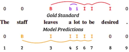
MWE identification is the task of determining, at the token level, which words are parts of MWEs, and which are not. For example, in the sentence
The staff leaves a lot to be desired (also used in
Figure 1) a lot and leaves to be desired are
MWEs. An important part of MWE identifica-tion is to be able to distinguish between MWEs and literal combinations that have the same surface
form; e.g., kick the bucket is ambiguous between
an idiomatic usage — meaning roughly ‘die’ — which is an MWE, and a literal one which is not. Many earlier studies on MWE identification have focused on this type of ambiguity, and treated the problem as one of word sense disambigua-tion, where literal and idiomatic usages are con-sidered different word senses (Birke and Sarkar, 2006; Katz and Giesbrecht, 2006; Li et al., 2010). Other work has leveraged linguistic knowledge of properties of MWEs in order to make these distinctions (Uchiyama et al., 2005; Fazly et al., 2009; Fothergill and Baldwin, 2012). Crucially, this work has typically focused on specific kinds of MWEs, and has not considered identification of the full spectrum of MWEs.
More-recent work has considered the identifica-tion of a wider range of types of MWEs. Brooke et al. (2014) present an unsupervised learning approach to segment a corpus into multiword units based on their predictability. Schneider et al. (2014a) propose methods for broad-coverage MWE identification, and evaluate them on a size-able corpus (Schneider et al., 2014b). They pro-posed a supervised learning approach based on the structured perceptron (Collins, 2002). The
sys-tem labels tokens using theBIOconvention, where
B indicates the beginning of an MWE, I
indi-cates the continuation of an MWE, and O
indi-cates that the token is not part of an MWE. The model includes features based on part-of-speech tags, MWE lexicons, and Brown clusters (Brown et al., 1992). Qu et al. (2015) later improved upon that system by using skip-gram embeddings (Mikolov et al., 2013) instead of Brown clus-ters with a variant of conditional random fields. More recently, Constant and Nivre (2016) incor-porate MWE identification along with dependency parsing by forming two representations for a sen-tence: a tree that represents the syntactic depen-dencies, and a forest of lexical trees that includes the MWEs identified in the sentence.
The recent SemEval shared task on Detect-ing Minimal Semantic Units and their MeanDetect-ings (DiMSUM) focused on MWE identification along with supersense tagging (Schneider et al., 2016). The best performing system for MWE identifica-tion for this shared task was that of Kirilin et al. (2016) which took into consideration all of the ba-sic features used by Schneider et al. (2014a) and two novel feature sets. The first one is based on the YAGO ontology (Suchanek et al., 2007), where heuristics were applied to extract potential named entities from the ontology. The second feature set was GloVe (Pennington et al., 2014) word embed-dings, with the word vectors scaled by a constant and divided by the standard deviation of each of its dimensions. None of the systems that partici-pated in the DiMSUM shared task considered deep learning approaches.
In this paper we propose the first deep learn-ing approaches to MWE identification. We use the DiMSUM data for training and evaluating our models, and compare against the state-of-the-art method of Kirilin et al. (2016). Here we focus solely on the MWE identification task, leaving su-persense tagging for future work.
3 Neural Network Models
In this section, we discuss the features extracted for the neural network models, and the model ar-chitectures. Schneider et al. (2014b) extracted roughly 320k sparse features. Because of the large input feature space, the only feasible way to train a model on those features is by using a linear clas-sifier. In contrast to Schneider et al. (2014b) our aim is to create dense input features to allow neu-ral network architectures, as well as other machine learning algorithms, to be trained on them. Specif-ically, we propose three neural network models: a layered feedforward network (LFN), a recurrent neural network (RNN), and a convolutional neural
network (CNN).1
3.1 Layered Feedforward Network
Although LFNs have been used to solve a wide range of classification and regression problems, they have been shown to be less effective for tasks at which deep learning models excel, such as im-age classification (Krizhevsky et al., 2012) and
machine translation (Bahdanau et al., 2015). The LFN is therefore proposed as a benchmark for comparing the performance of the other architec-tures, as well as for developing informative input features. Most feature engineering was carried out while developing this model and then transferred to the other architectures.
The composition of the DiMSUM corpus (Schneider et al., 2016), and the token-level lemma and part-of-speech annotations it provides, influenced our feature extraction. Most of the text in the DiMSUM corpus is social media text. The tokens and lemmas were therefore preprocessed
by removing#characters from tokens and lemmas
that contain them, and mapping URLs, numbers,
and any token or lemma containing the@symbol
to the special tokensURL,NUMBER, andUSER,
respectively. After pre-processing, distributed rep-resentations of all tokens and lemmas were ob-tained from a skip-gram (Mikolov et al., 2013) model. Specifically, the gensim ( ˇReh˚uˇrek and Sojka, 2010) implementation of skip-gram was trained on a snapshot of Wikipedia from Septem-ber 2015 to learn 100 dimensional word embed-dings. Any token occurring less than 15 times was discarded, the context window was set to 5, the negative sampling rate was set to 5, and un-known tokens were represented with a zero vector. The part-of-speech tag for each token was also en-coded, in this case as a one-hot vector.
Schneider et al. (2014a) included word shape features, which can be informative for the iden-tification of MWEs, especially named entities. We therefore also include word shape features. These are binary features for each token and lemma that capture whether it includes single or double quotes; consists of all capital letters; starts with a capital letter (but is otherwise lowercase);
con-tains a number; includes a# or@character;
cor-responds to a URL; contains any punctuation; and consists entirely of punctuation characters.
Schneider et al. (2014a) include features based on MWE lexicons that represent which tokens and lemmas are potentially part of an MWE and ac-cording to which lexicon. We use a script provided by Schneider et al. (2014a) to include these same features in our representation.
Finally, Salton et al. (2016) showed that embed-ding the entire sentence in which a target MWE occurs was helpful for distinguishing idiomatic from literal verb–noun idiomatic combinations.
We therefore also include a representation for the entire sentence. Specifically, we separately aver-age the skip-gram embeddings for the tokens and lemmas in the sentence containing the target word. These features were then input into an LFN model with a single hidden layer, which we refer to as LFN1.
3.2 Recurrent Neural Network
RNNs are a natural fit for many NLP problems due to their ability to model sequences. Here we apply an RNN to broad coverage MWE identification. The token for the current time step is represented using the same features as LFN1 described above, except we do not include the average of the skip-gram representations for tokens and lemmas in the same sentence as the target word because we ex-pect the RNN to be able to learn a representation of the sentence by itself. We use a single layer RNN model, referred to as RNN1.
3.3 Convolutional Neural Network
CNNs have been shown to be powerful classifiers (Kim, 2014; Kim et al., 2016), and since MWE identification can be formulated as a classification task, CNNs have the potential to perform well on it. The feature representation for the CNN was split into feature columns to enable the implemen-tation of the convolution layer. Each feature col-umn contains the same features as those for the RNN at each time step but since the CNN does not learn sequential information, a window of feature columns was given as an input.
4 Data and Evaluation
This section presents the statistics and structure of the dataset used for this task, as well as the evalu-ation methodology.
4.1 Dataset
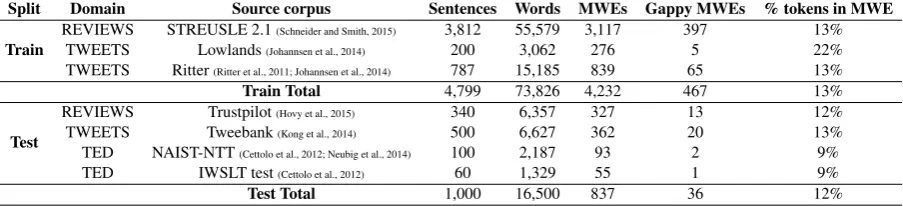
We use the DiMSUM dataset (Schneider et al., 2016) for our experiments, which allows for direct comparison with previous results. Table 1 displays the source corpora from which the dataset was constructed; their domain (i.e., reviews, tweets, or TED talks); the number of sentences, words, MWEs, and gappy (i.e., discontiguous) MWES in each source corpus; and the percentage of tokens belonging to an MWE in each source corpus. The dataset is split into training and testing sets such that the testing data contains a novel text type, i.e., TED talks.
For parameter tuning purposes, we also require validation data. We form a validation set from the training data by splitting the training data to cre-ate 5 folds, where every fold contained 20% vali-dation data, and the remaining 80% was used for training.
4.2 Structure
Every line in the dataset provides 8 pieces of in-formation: the numeric position of the token in its sentence; the token itself; its lemmatized form; its part-of-speech tag; its gold-standard MWE tag; the position of the last token that is part of its
MWE; its supersense tag;2 and the sentence ID.
Six MWE tags are used for MWE identification
in this dataset,Bwhich indicates the beginning of
an MWE,Iwhich indicates the continuation of an
MWE,Owhich indicates that the token is not part
of an MWE, b indicates the beginning of a new
MWE inside an MWE, iindicates the
continua-tion of the new MWE inside an MWE, and finally,
oindicates that the token that is inside an MWE is
not part of the nested MWE. This convention as-sumes that MWEs can only be nested to a depth of one (i.e., an MWE inside an MWE), and that MWEs must be properly nested.
4.3 Performance Metric
We use the link-based F-score evaluation met-ric from Schneider et al. (2014a), which allows
[image:4.595.309.526.62.150.2]2Schneider et al. (2014a) consider MWE identification and super-sense tagging. We focus only on MWE identifica-tion in this work and so don’t use the super-sense tag infor-mation provided in the dataset.
Figure 1: An example of how a model could tag a sequence, along with its gold standard tagging (adapted from Schneider et al. (2016)).
for direct comparison with prior work. Table 1 shows that the percentage of tokens occurring in MWEs ranges from 9–22%. As such, MWEs oc-cur much less frequently than literal word combi-nations. This evaluation metric correspondingly puts more emphasis on the ability of the model to detect MWEs rather than literal word combi-nations.
Figure 1 is a diagram adapted from Schneider et al. (2016) which shows an example of how a model could tag a sequence, as well as its gold standard tagging. The MWE tags on top represent the gold standard, and the MWE tags predicted by a system are shown on the bottom. A link is de-fined as the path from one token to another, as in Figure 1, regardless of the number of tokens in that path. Precision is calculated as the ratio of the number of correctly predicted links to the total number of links predicted by the model. Recall is calculated in the same way but swapping the gold standard and predicted links.
For example, in Figure 1, the model was able to correctly predict two links. The first link goes
frombtoiin the gold standard which is matched
by a predicted link from token 4–5 by the model. The second link is from token 6–7 in the gold stan-dard which matches the model’s prediction. Since the model predicted five links in total, the preci-sion is 25.
To calculate recall, the roles of the gold standard and model predictions are reversed. This way, three links have been correctly predicted. Two of the three links are the previously mentioned links.
The third one is the link fromB toIin the gold
standard which corresponds to the path from to-ken 3–6. Because there are four links in the gold
standard, the recall is therefore 3
4.
Split Domain Source corpus Sentences Words MWEs Gappy MWEs % tokens in MWE
Train REVIEWS STREUSLE 2.1
(Schneider and Smith, 2015) 3,812 55,579 3,117 397 13%
TWEETS Lowlands(Johannsen et al., 2014) 200 3,062 276 5 22%
TWEETS Ritter(Ritter et al., 2011; Johannsen et al., 2014) 787 15,185 839 65 13%
Train Total 4,799 73,826 4,232 467 13%
Test
REVIEWS Trustpilot(Hovy et al., 2015) 340 6,357 327 13 12%
TWEETS Tweebank(Kong et al., 2014) 500 6,627 362 20 13%
TED NAIST-NTT(Cettolo et al., 2012; Neubig et al., 2014) 100 2,187 93 2 9%
TED IWSLT test(Cettolo et al., 2012) 60 1,329 55 1 9%
[image:5.595.74.526.64.167.2]Test Total 1,000 16,500 837 36 12%
Table 1: Statistics describing the composition of the DiMSUM dataset.
1
F =
1 2(
1
P +
1
R) (1)
whereFis the F-score, andP andRare precision
and recall, respectively.
5 Parameter Settings
In this section, the architecture and parameters of all neural network models are presented in detail. The cost function used to train the neural network models was based on the cost function used by Schneider et al. (2014a) for this task:
cost= |y¯i|
X
i=1
c( ¯yi, yi) (2)
wherey¯iis theith gold standard MWE tag, andyi
is the ith MWE tag predicted by the neural
net-work model. To ensure that the MWE tag pre-dicted by the neural network is a probability dis-tribution, the output layer of all neural models was
the softmax layer. The functioncin Equation 2 is
defined as:
c( ¯yi, yi) = ¯yilog(yi) +ρ( ¯yi{B} ∧yi{O}) (3)
Some MWE tag sequences are invalid, for
ex-ample, a B followed immediately by an O
(be-cause MWEs are composed of multiple tokens),
and similarly, anOcannot occur immediately
be-fore an I(because the beginning of every MWE
must be tagged with a B). We therefore use the
Viterbi algorithm on the output of the neural net-work models to obtain the valid MWE tag se-quence with the highest probability. In prelimi-nary experiments we observed that setting all valid
transitions to be of equal probability, and the prob-ability of all invalid transitions to 0, performed best, and therefore use this strategy.
5.1 Layered Feedforward Network
The LFN was used as a benchmark neural network model against which the performance of the other deep learning models was compared. The param-eters that had to be tuned for this model were the size of the context window, the
misclassifica-tion penaltyρ(in Equation 3), the number of
neu-rons in each hidden layer, the number of iterations before training is stopped, and the dropout rate. Optimizing these parameters is important as they greatly influence the performance of the LFN. For all models considered, all parameter tuning was done using the validation data; the test data was never used for setting parameters.
Context window of sizes of 1, 2, and 3 tokens to the left and right were considered. A larger con-text window allows the model to see additional to-kens, but also makes the training process longer
and more prone to overfitting. In the case of ρ,
we investigated setting it between 40 and 100. A
small value of ρ would cause the model to have
decreases the association between neurons. It also has the same effect as ensembling multiple neu-ral network models because different neurons are switched on and off in every training iteration. The dropout rates that we considered ranged from 0.4 to 0.6.
After running multiple experiments, the best performing LFN model (LFN1) had a context win-dow of size 1, which means that the features for the tokens before and after the target token were input into the LFN along with the features of the
target token. The value of ρ was set to 50, and
the LFN had a single hidden layer containing 1000
neurons with the tanh activation function. The
LFN was trained for 1000 iterations with a dropout rate of 0.5.
5.2 Recurrent Neural Network
As previously mentioned in Section 3.2, RNNs are a natural fit to many NLP problems due to their ability to model sequences. At each timestep, the features for a token were input into the RNN which then output the corresponding MWE tag for that token. Many of the parameters that had to be tuned for the LFN had to be tuned for the RNN
as well: ρ ranged from 10 to 50; the number of
neurons in each hidden layer ranged from 50 to 300; the dropout rate ranged from 0.5 to 1; and we again tuned the number of iterations before
train-ing is stopped.3 Parameters specific to the RNN
model that had to be tuned include whether the RNN is unidirectional or bidirectional, and the cell type, where we consider a fully connected RNN, an LSTM cell, and a GRU cell.
After observing the performance of the RNN on the validation set, the best performing RNN
model (RNN1) was a bidirectional LSTM withρ
set to 25, with a single hidden layer containing 100 neurons. It was trained for 60 iterations with no dropout. This indicates that the LSTM cell was able to handle the complexity of the sequences of tokens without requiring regularization.
As we will see in Section 6, RNN1 unfortu-nately did not perform as well as the other neu-ral network models. We therefore attempted to improve its performance using two additional ap-proaches. In the first approach, the RNN LSTM was orthogonally initialized. Saxe et al. (2014) showed that orthogonally initializing RNNs led to
3We choose parameter settings to explore based on per-formance on the validation data, and so consider different pa-rameter settings here than for LFN1.
better learning in deep neural networks. Never-theless, orthogonal initialization did not seem to have an effect on the performance of RNN1. In the second approach, the dataset was artificially expanded by splitting the input sentences on punc-tuation. This provided more “sentences” for the RNN LSTM to learn from, but again did not im-prove performance.
5.3 Convolutional Neural Network
Every token was represented by a feature column and these feature columns were then concatenated to form the input to the CNN. A convolutional layer was then applied to the input and then max-pooled to form the hidden layer which was used to produce the predicted output. There were again many parameters to optimize in the CNN. We con-sidered the same settings for the context window size as for LFN1, i.e., 1, 2, and 3 tokens to the left and right. The number of neurons in each hid-den layer ranged from 25 to 200. In contrast to LFN1 and RNN1, here we consider varying num-bers of fully connected hidden layers from 1–3. The dropout rate at the fully connected layers, as well as the convolutional layer, ranged from 0.3 to
1, andρranged from 10 to 30. Parameters specific
to the convolutional neural network that were op-timized were the number of filters, which ranged from 100 to 500, and spanned 1, 2, or 3 feature columns, and the types of convolution and pooling operations that were performed. Having a large number of filters can cause the network to pick up noise patterns which makes the CNN overfit. The size of the filters and the types of convolution and pooling operations is largely dependent on the data and were optimized according to the performance of the model on the validation set.
We experiment with two CNN models, the best performing CNN model with two hidden layers (CNN2) and the best performing CNN model with three hidden layers (CNN3). CNN2 was trained for 600 iterations and had a context window of size
1 andρequal to 20, with 250 filters that spanned
CNN3 is similar to CNN2 but was trained for 900 iterations and had the 450 neuron hidden layer feed to a hidden layer containing 100 neurons with the sigmoid activation function. The output of that layer was then passed to another layer containing
50 neurons with the tanh activation function
be-fore being passed to the output softmax layer. The
intuition behind the tanh activation function for
the last hidden layer is that the layer before it has the sigmoid activation function. This means that the values that are passed to the last hidden layer are between 0 and 1 multiplied by the weights be-tween the two layers. Since these weights can be negative, a sigmoid function that can deal with
negative values is required, and thetanhfunction
satisfies this requirement. Both models have a dropout rate of 60% on the convolutional and hid-den layers. They were also given batches of 6000 random examples at each training iteration.
5.4 Traditional Machine Learning Models
To demonstrate the effectiveness of neural net-work models, we compare them against more-traditional, non-neural machine learning models.
Here we consider k-nearest neighbour, random
forests, logistic regression, and gradient boosting.4
These models were given the same features that were input into LFN1, and parameter tuning was
also carried out on the validation set. For the k
-nearest neighbour algorithm, kwas set to 3, and
the points were weighted by the inverse of their distance. For random forests, 100 estimators were used while multiplying the penalty of
misclassify-ing any class other thanOasOby 1.2. In the case of
logistic regression, L2 regularization was utilized with a regularization factor of 0.5. For gradient boosting, 100 estimators with a maximum depth of 13 nodes were used. Using a larger number of estimators for random forest and gradient boost-ing has shown to improve their cross validation performance. However, the point of diminishing returns was found to be at around 50 estimators, and it was clear that increasing the number of esti-mators above 100 would not yield any significant increase in performance. Added to that, with gra-dient boosting, the cross validation performance also increased with the maximum node depth, but the point of diminishing returns was found to be at around 9, and it was clear that increasing the
4In preliminary experiments we also considered an SVM, but found the training time to be impractical, and so did not consider it further.
maximum depth beyond 13 would not yield any significant increase in performance.
5.5 Implementation Details
Overall, 983 features were input into the LFN and traditional machine learning models, and more than 50 parameter combinations were examined. Every LFN model required up to 2 days of train-ing. For the RNN, every token was represented by a feature vector of length 257, and took around 10 hours to train. More than 30 parameter combi-nations were examined for the RNN model. Ev-ery feature column in the CNN model contained 257 features, this amounts to a total of 771 input features. More than 130 parameter combinations were tested for the CNN, and it required around 12 hours of training. Tensorflow (et al., 2015) ver-sion 0.12 was used to implement the neural net-work models, and scikit-learn (Pedregosa et al., 2011) was used to implement the traditional ma-chine learning models. The experiments were run on 2 GHz Intel Xeon E7-4809 v3 CPUs.
6 Results
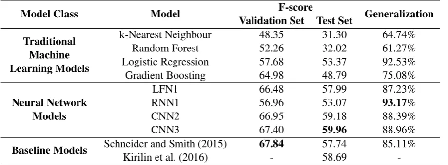
The average F-score of the models on the five fold cross validation set, and their F-score on the test set, along with their generalization, is shown in Table 2. All models except for that of Kirilin et al. (2016) — which was already optimized for this task by its authors — were run on the validation set to tune their parameters. To evaluate the per-formance of the models on the test set, the models were trained on the entire training set (which in-cludes the validation splits) and then tested on the test set.
We first consider the traditional machine learn-ing models. Amongst these models, gradient boosting performed best on the validation set, which can be attributed to the ability of gradient boosting to learn complex functions and its ro-bustness to outliers. However, it did not perform as well on the test set, where logistic regression performed best, and achieved the best generaliza-tion out of the tradigeneraliza-tional machine learning mod-els. This shows that relatively many instances in the test set can be correctly classified by using a hyperplane to separate the dense feature represen-tations.
Model Class Model Validation Set Test SetF-score Generalization
Traditional Machine Learning Models
k-Nearest Neighbour 48.35 31.30 64.74%
Random Forest 52.26 32.02 61.27%
Logistic Regression 57.68 53.37 92.53%
Gradient Boosting 64.98 48.79 75.08%
Neural Network Models
LFN1 66.48 57.99 87.23%
RNN1 56.96 53.07 93.17%
CNN2 66.95 59.18 88.39%
CNN3 67.40 59.96 88.96%
Baseline Models Schneider and Smith (2015)Kirilin et al. (2016) 67.84- 57.7458.69 85.11%
-Table 2: The average F-score of each model on the 5 fold cross validation set, and their F-score on the test set, along with their generalization. The best performance in each column is shown in boldface.
comes close to the previous state-of-the-art of Kir-ilin et al. (2016). RNN1 achieved the best gener-alization out of all models considered; however, it performed relatively poorly compared to the other neural network models on both the validation and test sets. The CNN models, CNN2 and CNN3, both improved over the previous best results on the test set — with CNN3 achieving the best F-score overall — and outperformed all other models ex-cept for (Schneider et al., 2014a) on the validation set. This shows that the CNN filters were able to learn what makes a feature column a part of an MWE or not. That CNN3 outperforms CNN2 fur-ther shows that adding an extra hidden layer for the CNN model improves its performance as it is able to handle more complex mappings. Moreover, the training data for this task is relatively small; it con-sists of less than 5,000 sentences. These results therefore further show that convolutional neural networks can still achieve good performance when the amount of training data available is limited.
The highest F-score on the test set — achieved by CNN3 — is 59.96. This shows that the task is quite difficult, and suggests that there is scope for further improvements. One issue, however, is that there are notable inconsistencies in the annotations
in the dataset. For example, the expressiona fewis
labeled as an MWE 15 out of 32 times in the train-ing set, even though there appears to be no vari-ation in its usage. Recent efforts have, however, proposed semi-automated methods for resolving these inconsistencies (Chan et al., 2017).
7 Conclusions and Future Work
We proposed and evaluated the first neural net-work approaches for multiword expression identi-fication, and compared their performance against the previous state-of-art, and more-traditional ma-chine learning approaches. We showed that our proposed approach based on a convolutional neu-ral network (CNN2 and CNN3) outperformed the previous state-of-the-art for this task. Therefore, although the task is inherently sequential, formu-lating it as a classification task enabled the CNN models to perform well on it. This finding sug-gests that deep learning methods can still be ef-fective when only limited amounts of training data are available. Furthermore, the proposed neural network-based approaches were able to generalize more-effectively than previous approaches.
[image:8.595.74.534.62.232.2]Acknowledgments
This work is financially supported by the Natu-ral Sciences and Engineering Research Council of Canada, the New Brunswick Innovation Founda-tion, and the University of New Brunswick.
References
Dzmitry Bahdanau, Kyunghyun Cho, and Yoshua Ben-gio. 2015. Neural machine translation by jointly learning to align and translate. InInternational Con-ference on Learning Representations (ICLR2015). Timothy Baldwin and Su Nam Kim. 2010. Handbook
of natural language processing. In Nitin Indurkhya and Fred J. Damerau, editors, Handbook of Natu-ral Language Processing, CRC Press, Boca Raton, USA. 2nd edition.
G´abor Berend. 2011. Opinion expression mining by exploiting keyphrase extraction. In Proceedings of 5th International Joint Conference on Natural Language Processing. Chiang Mai, Thailand, pages 1162–1170.
Julia Birke and Anoop Sarkar. 2006. A clustering ap-proach for nearly unsupervised recognition of non-literal language. In Proceedings of the 11th Con-ference of the European Chapter of the Associa-tion for ComputaAssocia-tional Linguistics (EACL-2006). Trento, Italy, pages 329–336.
Julian Brooke, Vivian Tsang, Graeme Hirst, and Fraser Shein. 2014. Unsupervised multiword segmentation of large corpora using prediction-driven decompo-sition of n-grams. In COLING 2014, 25th Inter-national Conference on Computational Linguistics, Proceedings of the Conference: Technical Papers. Dublin, Ireland, pages 753–761.
Peter F. Brown, Vincent J. Della Pietra, Peter V. de Souza, Jennifer C. Lai, and Robert L. Mercer. 1992. Class-based n-gram models of natural lan-guage. Computational Linguistics18(4):467–479.
Marine Carpuat and Mona Diab. 2010. Task-based evaluation of multiword expressions: a pilot study in statistical machine translation. In Human Lan-guage Technologies: The 2010 Annual Conference of the North American Chapter of the Association for Computational Linguistics. Los Angeles, Cali-fornia, pages 242–245.
Mauro Cettolo, Christian Girardi, and Marcello Fed-erico. 2012. Web inventory of transcribed and trans-lated talks. InProceedings of the 16th Annual Con-ference of the European Association for Machine Translation (EAMT 2012). Trento, Italy, pages 261– 268.
King Chan, Julian Brooke, and Timothy Baldwin. 2017. Semi-automated resolution of inconsistency
for a harmonized multiword expression and depen-dency parse annotation. InProceedings of the 13th Workshop on Multiword Expressions (MWE 2017). Valencia, Spain, pages 187–193.
Kyunghyun Cho, Bart van Merrienboer, C¸aglar G¨ulc¸ehre, Dzmitry Bahdanau, Fethi Bougares, Hol-ger Schwenk, and Yoshua Bengio. 2014. Learning phrase representations using RNN encoder-decoder for statistical machine translation. InProceedings of the 2014 Conference on Empirical Methods in Nat-ural Language Processing, A meeting of SIGDAT, a Special Interest Group of the ACL. Doha, Qatar, pages 1724–1734.
Michael Collins. 2002. Discriminative training meth-ods for hidden markov models: Theory and exper-iments with perceptron algorithms. In Proceed-ings of the 2002 Conference on Empirical Methods in Natural Language Processing (EMNLP 2002). Philadelphia, USA, pages 1–8.
Matthieu Constant and Joakim Nivre. 2016. A transition-based system for joint lexical and syn-tactic analysis. InProceedings of the 54th Annual Meeting of the Association for Computational Lin-guistics. Berlin, Germany, pages 161–171.
Mart´ın Abadi et al. 2015. TensorFlow: Large-scale machine learning on heterogeneous sys-tems. Software available from tensorflow.org. http://tensorflow.org/.
Afsaneh Fazly, Paul Cook, and Suzanne Stevenson. 2009. Unsupervised type and token identification of idiomatic expressions. Computational Linguis-tics35(1):61–103.
Richard Fothergill and Timothy Baldwin. 2012. Com-bining resources for mwe-token classification. In
*SEM 2012: The First Joint Conference on Lexical and Computational Semantics – Volume 1: Proceed-ings of the main conference and the shared task, and Volume 2: Proceedings of the Sixth International Workshop on Semantic Evaluation (SemEval 2012). Montr´eal, Canada, pages 100–104.
Dirk Hovy, Anders Johannsen, and Anders Søgaard. 2015. User review sites as a resource for large-scale sociolinguistic studies. InProceedings of the 24th International Conference on World Wide Web. Flo-rence, Italy, pages 452–461.
Anders Johannsen, Dirk Hovy, H´ector Mart´ınez Alonso, Barbara Plank, and Anders Søgaard. 2014. More or less supervised supersense tagging of twitter. In Proceedings of the Third Joint Conference on Lexical and Computational Semantics (*SEM 2014). Dublin, Ireland, pages 1–11.
Proceedings of the Workshop on Multiword Expres-sions: Identifying and Exploiting Underlying Prop-erties. Sydney, Australia, pages 12–19.
Yoon Kim. 2014. Convolutional neural networks for sentence classification. InProceedings of the 2014 Conference on Empirical Methods in Natural Lan-guage Processing, EMNLP, A meeting of SIGDAT, a Special Interest Group of the ACL. Doha, Qatar, pages 1746–1751.
Yoon Kim, Yacine Jernite, David Sontag, and Alexan-der M. Rush. 2016. Character-aware neural lan-guage models. InProceedings of the Thirtieth AAAI Conference on Artificial Intelligence. Phoenix, Ari-zona, USA, pages 2741–2749.
Angelika Kirilin, Felix Krauss, and Yannick Versley. 2016. ICL-HD at semeval-2016 task 10: Improv-ing the detection of minimal semantic units and their meanings with an ontology and word embeddings. In Proceedings of the 10th International Workshop on Semantic Evaluation, SemEval@NAACL-HLT. San Diego, CA, USA, pages 937–945.
Lingpeng Kong, Nathan Schneider, Swabha Swayamdipta, Archna Bhatia, Chris Dyer, and Noah A. Smith. 2014. A dependency parser for tweets. InProceedings of the 2014 Conference on Empirical Methods in Natural Language Process-ing, A meeting of SIGDAT, a Special Interest Group of the ACL. Doha, Qatar, pages 1001–1012.
Alex Krizhevsky, Ilya Sutskever, and Geoffrey E Hin-ton. 2012. ImageNet classification with deep con-volutional neural networks. In F. Pereira, C. J. C. Burges, L. Bottou, and K. Q. Weinberger, editors,
Advances in Neural Information Processing Systems 25, Curran Associates, Inc., pages 1097–1105.
Guillaume Lample, Miguel Ballesteros, Sandeep Sub-ramanian, Kazuya Kawakami, and Chris Dyer. 2016. Neural architectures for named entity recognition. In NAACL HLT 2016, The 2016 Conference of the North American Chapter of the Association for Computational Linguistics: Human Language Tech-nologies. San Diego, California, USA, pages 260– 270.
Jiwei Li, Minh-Thang Luong, and Dan Jurafsky. 2015. A hierarchical neural autoencoder for paragraphs and documents. InProceedings of the 53rd Annual Meeting of the Association for Computational Lin-guistics and the 7th International Joint Conference on Natural Language Processing of the Asian Feder-ation of Natural Language Processing, ACL, Volume 1: Long Papers. Beijing, China, pages 1106–1115.
Linlin Li, Benjamin Roth, and Caroline Sporleder. 2010. Topic models for word sense disambiguation and token-based idiom detection. In Proceedings of the 48th Annual Meeting of the Association for Computational Linguistics. Uppsala, Sweden, pages 1138–1147.
Tomas Mikolov, Ilya Sutskever, Kai Chen, Greg S Cor-rado, and Jeff Dean. 2013. Distributed representa-tions of words and phrases and their composition-ality. In C. J. C. Burges, L. Bottou, M. Welling, Z. Ghahramani, and K. Q. Weinberger, editors, Ad-vances in Neural Information Processing Systems 26, Curran Associates, Inc., pages 3111–3119.
Graham Neubig, Katsuhito Sudoh, Yusuke Oda, Kevin Duh, Hajime Tsukada, and Masaaki Nagata. 2014. The NAIST-NTT TED talk treebank. In Interna-tional Workshop on Spoken Language Translation (IWSLT). Lake Tahoe, USA.
David Newman, Nagendra Koilada, Jey Han Lau, and Timothy Baldwin. 2012. Bayesian text segmenta-tion for index term identificasegmenta-tion and keyphrase ex-traction. InProceedings of COLING 2012. Mumbai, India, pages 2077–2092.
F. Pedregosa, G. Varoquaux, A. Gramfort, V. Michel, B. Thirion, O. Grisel, M. Blondel, P. Pretten-hofer, R. Weiss, V. Dubourg, J. Vanderplas, A. Pas-sos, D. Cournapeau, M. Brucher, M. Perrot, and E. Duchesnay. 2011. Scikit-learn: Machine learning in Python. Journal of Machine Learning Research
12:2825–2830.
Jeffrey Pennington, Richard Socher, and Christopher Manning. 2014. Glove: Global vectors for word representation. In Proceedings of the 2014 Con-ference on Empirical Methods in Natural Language Processing (EMNLP). Doha, Qatar, pages 1532– 1543.
Lizhen Qu, Gabriela Ferraro, Liyuan Zhou, Wei-wei Hou, Nathan Schneider, and Timothy Baldwin. 2015. Big data small data, in domain out-of domain, known word unknown word: The impact of word representations on sequence labelling tasks. In Pro-ceedings of the Nineteenth Conference on Computa-tional Natural Language Learning. Beijing, China, pages 83–93.
Radim ˇReh˚uˇrek and Petr Sojka. 2010. Software Frame-work for Topic Modelling with Large Corpora. In
Proceedings of the LREC 2010 Workshop on New Challenges for NLP Frameworks. Valletta, Malta, pages 45–50.
Alan Ritter, Sam Clark, Mausam, and Oren Etzioni. 2011. Named entity recognition in tweets: An ex-perimental study. InProceedings of the 2011 Con-ference on Empirical Methods in Natural Language Processing, A meeting of SIGDAT, a Special Inter-est Group of the ACL. Edinburgh, UK, pages 1524– 1534.
Giancarlo Salton, Robert Ross, and John Kelleher. 2016. Idiom token classification using sentential distributed semantics. In Proceedings of the 54th Annual Meeting of the Association for Computa-tional Linguistics (Volume 1: Long Papers). Berlin, Germany, pages 194–204.
Andrew M. Saxe, James L. McClelland, and Surya Ganguli. 2014. Exact solutions to the nonlinear dy-namics of learning in deep linear neural networks. InInternational Conference on Learning Represen-tations (ICLR2014).
Nathan Schneider, Emily Danchik, Chris Dyer, and A. Noah Smith. 2014a. Discriminative lexical se-mantic segmentation with gaps: Running the mwe gamut. Transactions of the Association for Compu-tational Linguistics (TACL)2:193–206.
Nathan Schneider, Dirk Hovy, Anders Johannsen, and Marine Carpuat. 2016. SemEval-2016 task 10: Detecting minimal semantic units and their meanings (DiMSUM). In Proceedings of the 10th International Workshop on Semantic Evalua-tion, SemEval@NAACL-HLT. San Diego, CA, USA, pages 546–559.
Nathan Schneider, Spencer Onuffer, Nora Kazour, Emily Danchik, Michael T. Mordowanec, Henrietta Conrad, and Noah A. Smith. 2014b. Comprehensive annotation of multiword expressions in a social web corpus. In Proceedings of the Ninth International Conference on Language Resources and Evaluation (LREC-2014). Reykjavik, Iceland, pages 455–461. Nathan Schneider and A. Noah Smith. 2015. A corpus
and model integrating multiword expressions and supersenses. InProceedings of the 2015 Conference of the North American Chapter of the Association for Computational Linguistics: Human Language Technologies. Denver, Colorado, pages 1537–1547. Nitish Srivastava, Geoffrey E. Hinton, Alex
Krizhevsky, Ilya Sutskever, and Ruslan Salakhutdi-nov. 2014. Dropout: a simple way to prevent neural networks from overfitting. Journal of Machine Learning Research15(1):1929–1958.
Fabian M. Suchanek, Gjergji Kasneci, and Gerhard Weikum. 2007. Yago: a core of semantic knowl-edge. InProceedings of the 16th International Con-ference on World Wide Web. Banff, Alberta, Canada, pages 697–706.
Ilya Sutskever, Oriol Vinyals, and Quoc V Le. 2014. Sequence to sequence learning with neural net-works. In Z. Ghahramani, M. Welling, C. Cortes, N. D. Lawrence, and K. Q. Weinberger, editors, Ad-vances in Neural Information Processing Systems 27, Curran Associates, Inc., pages 3104–3112. Kiyoko Uchiyama, Timothy Baldwin, and Shun