Chunking with Support Vector Machines
Taku Kudo and Yuji Matsumoto
Graduate School of Information Science, Nara Institute of Science and Technology
taku-ku,matsu @is.aist-nara.ac.jp
Abstract
We apply Support Vector Machines (SVMs) to identify English base phrases (chunks). SVMs are known to achieve high generalization perfor-mance even with input data of high dimensional feature spaces. Furthermore, by the Kernel princi-ple, SVMs can carry out training with smaller com-putational overhead independent of their dimen-sionality. We apply weighted voting of 8 SVMs-based systems trained with distinct chunk repre-sentations. Experimental results show that our proach achieves higher accuracy than previous ap-proaches.
1 Introduction
Chunking is recognized as series of processes — first identifying proper chunks from a sequence of tokens (such as words), and second classifying these chunks into some grammatical classes. Various NLP tasks can be seen as a chunking task. Exam-ples include English base noun phrase identification (base NP chunking), English base phrase identifica-tion (chunking), Japanese chunk (bunsetsu) identi-fication and named entity extraction. Tokenization and part-of-speech tagging can also be regarded as a chunking task, if we assume each character as a token.
Machine learning techniques are often applied to chunking, since the task is formulated as estimating an identifying function from the information (fea-tures) available in the surrounding context. Various machine learning approaches have been proposed for chunking (Ramshaw and Marcus, 1995; Tjong Kim Sang, 2000a; Tjong Kim Sang et al., 2000; Tjong Kim Sang, 2000b; Sassano and Utsuro, 2000; van Halteren, 2000).
Conventional machine learning techniques, such as Hidden Markov Model (HMM) and Maximum Entropy Model (ME), normally require a careful feature selection in order to achieve high accuracy.
They do not provide a method for automatic selec-tion of given feature sets. Usually, heuristics are used for selecting effective features and their com-binations.
New statistical learning techniques such as Sup-port Vector Machines (SVMs) (Cortes and Vap-nik, 1995; VapVap-nik, 1998) and Boosting(Freund and Schapire, 1996) have been proposed. These tech-niques take a strategy that maximizes the margin between critical samples and the separating hyper-plane. In particular, SVMs achieve high generaliza-tion even with training data of a very high dimen-sion. Furthermore, by introducing the Kernel func-tion, SVMs handle non-linear feature spaces, and carry out the training considering combinations of more than one feature.
In the field of natural language processing, SVMs are applied to text categorization and syntactic de-pendency structure analysis, and are reported to have achieved higher accuracy than previous ap-proaches.(Joachims, 1998; Taira and Haruno, 1999; Kudo and Matsumoto, 2000a).
In this paper, we apply Support Vector Machines to the chunking task. In addition, in order to achieve higher accuracy, we apply weighted voting of 8 SVM-based systems which are trained using dis-tinct chunk representations. For the weighted vot-ing systems, we introduce a new type of weightvot-ing strategy which are derived from the theoretical basis of the SVMs.
2 Support Vector Machines 2.1 Optimal Hyperplane
Let us define the training samples each of which belongs either to positive or negative class as:
! #"%$&$'#(
)
is a feature vector of the *-th sample
repre-sented by an + dimensional vector. is the class
(positive(
"%$
) or negative(
&$
) class) label of the *
sam-Small Margin Large Margin
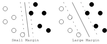
Figure 1: Two possible separating hyperplanes
ples. In the basic SVMs framework, we try to sep-arate the positive and negative samples by a hyper-plane expressed as:
-/.(0"2143656-78901:
;
. SVMs find an “optimal” hyperplane (i.e. an optimal parameter set for
-<=1
) which separates the training data into two classes. What does “optimal” mean? In order to define it, we need to consider the margin between two classes. Figure 1 illus-trates this idea. Solid lines show two possible hyper-planes, each of which correctly separates the train-ing data into two classes. Two dashed lines paral-lel to the separating hyperplane indicate the bound-aries in which one can move the separating hyper-plane without any misclassification. We call the dis-tance between those parallel dashed lines as
mar-gin. SVMs find the separating hyperplane which
maximizes its margin. Precisely, two dashed lines and margin (> ) can be expressed as:
-?.@"A1B3
C
$D
>
36EDFHG-JI
.
To maximize this margin, we should minimize
I=-KI
. In other words, this problem becomes equiva-lent to solving the following optimization problem:
LNMPOQMSRTMVUW9X Y
-Z[3
\
I]-JI
\
^`_`aQb
Wcd8dfe9X
fgh-i.)j)"21lkm6$
*
3n$D
,
The training samples which lie on either of two dashed lines are called support vectors. It is known that only the support vectors in given training data matter. This implies that we can obtain the same de-cision function even if we remove all training sam-ples except for the extracted support vectors.
In practice, even in the case where we cannot sep-arate training data linearly because of some noise in the training data, etc, we can build the sep-arating linear hyperplane by allowing some mis-classifications. Though we omit the details here, we can build an optimal hyperplane by introducing a soft margin parametero , which trades off between
the training error and the magnitude of the margin. Furthermore, SVMs have a potential to carry out the non-linear classification. Though we leave the
details to (Vapnik, 1998), the optimization problem can be rewritten into a dual form, where all feature vectors appear in their dot products. By simply sub-stituting every dot product of
)
and
0p
in dual form with a certain Kernel functionq
rf0p
, SVMs can handle non-linear hypotheses. Among many kinds of Kernel functions available, we will focus on the
s
-th polynomial kernel: q
t)rfuplv3w)D.x0py"z$f{
. Use of
s
-th polynomial kernel functions allows us to build an optimal separating hyperplane which takes into account all combinations of features up to
s
.
2.2 Generalization Ability of SVMs
Statistical Learning Theory(Vapnik, 1998) states that training error (empirical risk)|:} and test error
(risk)|~ hold the following theorem.
Theorem 1 (Vapnik) If
N6,
is the VC dimen-sion of the class functions implemented by some ma-chine learning algorithms, then for all functions of that class, with a probability of at least
$&
, the risk is bounded by
|~ |
}
"6
O
\
"6$[&K
O%
,
(1)
where is a non-negative integer called the Vapnik
Chervonenkis (VC) dimension, and is a measure of the complexity of the given decision function. The r.h.s. term of (1) is called VC bound. In order to minimize the risk, we have to minimize the empir-ical risk as well as VC dimension. It is known that the following theorem holds for VC dimension
and margin> (Vapnik, 1998).
Theorem 2 (Vapnik) Suppose + as the dimension
of given training samples> as the margin, and
as the smallest diameter which encloses all train-ing sample, then VC dimension of the SVMs are
bounded by
R%MPO
\
F
>
\
+
"!$
(2)
In order to minimize the VC dimension , we have
to maximize the margin > , which is exactly the
strategy that SVMs take.
Vapnik gives an alternative bound for the risk.
Theorem 3 (Vapnik) Suppose |
is an error rate estimated by Leave-One-Out procedure, |
is bounded as
|
N
19
DD
#)%=#
14%#
*r+0*x+`
,
Leave-One-Out procedure is a simple method to ex-amine the risk of the decision function — first by removing a single sample from the training data, we construct the decision function on the basis of the remaining training data, and then test the removed sample. In this fashion, we test all, samples of the
training data using, different decision functions. (3)
is a natural consequence bearing in mind that sup-port vectors are the only factors contributing to the final decision function. Namely, when the every re-moved support vector becomes error in Leave-One-Out procedure,|
becomes the r.h.s. term of (3). In practice, it is known that this bound is less predic-tive than the VC bound.
3 Chunking
3.1 Chunk representation
There are mainly two types of representations for proper chunks. One is Inside/Outside representa-tion, and the other is Start/End representation.
1. Inside/Outside
This representation was first introduced in (Ramshaw and Marcus, 1995), and has been applied for base NP chunking. This method uses the following set of three tags for repre-senting proper chunks.
I Current token is inside of a chunk. O Current token is outside of any chunk. B Current token is the beginning of a chunk
which immediately follows another chunk. Tjong Kim Sang calls this method as IOB1 representation, and introduces three alternative versions — IOB2,IOE1 and IOE2 (Tjong Kim Sang and Veenstra, 1999).
IOB2 A B tag is given for every token which exists at the beginning of a chunk. Other tokens are the same as IOB1. IOE1 An E tag is used to mark the last
to-ken of a chunk immediately preceding another chunk.
IOE2 An E tag is given for every token which exists at the end of a chunk. 2. Start/End
This method has been used for the Japanese named entity extraction task, and requires the following five tags for representing proper chunks(Uchimoto et al., 2000)1.
1Originally, Uchimoto uses C/E/U/O/S representation.
However we rename them as B/I/O/E/S for our purpose, since
IOB1 IOB2 IOE1 IOE2 Start/End
In O O O O O
early I B I I B
trading I I I E E
in O O O O O
busy I B I I B
Hong I I I I I
Kong I I E E E
Monday B B I E S
, O O O O O
gold I B I E S
[image:3.612.318.538.72.224.2]was O O O O O
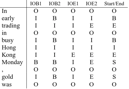
Table 1: Example for each chunk representation
B Current token is the start of a chunk con-sisting of more than one token.
E Current token is the end of a chunk consist-ing of more than one token.
I Current token is a middle of a chunk con-sisting of more than two tokens.
S Current token is a chunk consisting of only one token.
O Current token is outside of any chunk.
Examples of these five representations are shown in Table 1.
If we have to identify the grammatical class of each chunk, we represent them by a pair of an I/O/B/E/S label and a class label. For example, in IOB2 representation, B-VP label is given to a to-ken which represents the beginning of a verb base phrase (VP).
3.2 Chunking with SVMs
Basically, SVMs are binary classifiers, thus we must extend SVMs to multi-class classifiers in order to classify three (B,I,O) or more (B,I,O,E,S) classes. There are two popular methods to extend a binary classification task to that ofq classes. One is one
class vs. all others. The idea is to build q
classi-fiers so as to separate one class from all others. The other is pairwise classification. The idea is to build
q¢¡
q
&!$fFDE
classifiers considering all pairs of classes, and final decision is given by their weighted voting. There are a number of other methods to ex-tend SVMs to multiclass classifiers. For example, Dietterich and Bakiri(Dietterich and Bakiri, 1995) and Allwein(Allwein et al., 2000) introduce a uni-fying framework for solving the multiclass problem
by reducing them into binary models. However, we employ the simple pairwise classifiers because of the following reasons:
(1) In general, SVMs require £
+
\
¥¤
£
+H¦
training cost (where + is the size of training data).
Thus, if the size of training data for individual bi-nary classifiers is small, we can significantly reduce the training cost. Although pairwise classifiers tend to build a larger number of binary classifiers, the training cost required for pairwise method is much more tractable compared to the one vs. all others.
(2) Some experiments (Kreßel, 1999) report that a combination of pairwise classifiers performs bet-ter than the one vs. all others.
For the feature sets for actual training and classi-fication of SVMs, we use all the information avail-able in the surrounding context, such as the words, their part-of-speech tags as well as the chunk labels. More precisely, we give the following features to identify the chunk label
=
for the*-th word:
§
Direction §
Word: ¨ ©
\
¨
©0
¨
¨
Pª
¨
Pª)
POS:
©
\
h©0 Pª) Pª
Chunk:
=©
\
=© =
Here,¨
is the word appearing at*-th position, r
is the POS tag of ¨
, and
=
is the (extended) chunk label for*-th word. In addition, we can reverse the
parsing direction (from right to left) by using two chunk tags which appear to the r.h.s. of the current token (
Pª) = Pª
\
). In this paper, we call the method which parses from left to right as forward parsing, and the method which parses from right to left as
backward parsing.
Since the preceding chunk labels (
©0=©
\
for forward parsing ,
=Pª=Pª
\
for backward parsing) are not given in the test data, they are decided dy-namically during the tagging of chunk labels. The technique can be regarded as a sort of Dynamic Pro-gramming (DP) matching, in which the best answer is searched by maximizing the total certainty score for the combination of tags. In using DP matching, we limit a number of ambiguities by applying beam search with width
. In CoNLL 2000 shared task, the number of votes for the class obtained through the pairwise voting is used as the certain score for beam search with width 5 (Kudo and Matsumoto, 2000a). In this paper, however, we apply determin-istic method instead of applying beam search with keeping some ambiguities. The reason we apply de-terministic method is that our further experiments
and investigation for the selection of beam width shows that larger beam width dose not always give a significant improvement in the accuracy. Given our experiments, we conclude that satisfying accuracies can be obtained even with the deterministic parsing. Another reason for selecting the simpler setting is that the major purpose of this paper is to compare weighted voting schemes and to show an effective weighting method with the help of empirical risk estimation frameworks.
3.3 Weighted Voting
Tjong Kim Sang et al. report that they achieve higher accuracy by applying weighted voting of sys-tems which are trained using distinct chunk rep-resentations and different machine learning algo-rithms, such as MBL, ME and IGTree(Tjong Kim Sang, 2000a; Tjong Kim Sang et al., 2000). It is well-known that weighted voting scheme has a potential to maximize the margin between critical samples and the separating hyperplane, and pro-duces a decision function with high generalization performance(Schapire et al., 1997). The boosting technique is a type of weighted voting scheme, and has been applied to many NLP problems such as parsing, part-of-speech tagging and text categoriza-tion.
In our experiments, in order to obtain higher ac-curacy, we also apply weighted voting of 8 SVM-based systems which are trained using distinct chunk representations. Before applying weighted voting method, first we need to decide the weights to be given to individual systems. We can obtain the best weights if we could obtain the accuracy for the “true” test data. However, it is impossible to estimate them. In boosting technique, the voting weights are given by the accuracy of the training data during the iteration of changing the frequency (distribution) of training data. However, we can-not use the accuracy of the training data for vot-ing weights, since SVMs do not depend on the fre-quency (distribution) of training data, and can sepa-rate the training data without any mis-classification by selecting the appropriate kernel function and the soft margin parameter. In this paper, we introduce the following four weighting methods in our exper-iments:
1. Uniform weights
2. Cross validation
Dividing training data into
portions, we em-ploy the training by using
&2$
portions, and then evaluate the remaining portion. In this fashion, we will have
individual accuracy. Final voting weights are given by the average of these
accuracies. 3. VC-bound
By applying (1) and (2), we estimate the lower bound of accuracy for each system, and use the accuracy as a voting weight. The voting weight is calculated as: ¨
3«$&
o
1
+
s
. The value of , which represents the smallest
diameter enclosing all of the training data, is approximated by the maximum distance from the origin.
4. Leave-One-Out bound
By using (3), we estimate the lower bound of the accuracy of a system. The voting weight is calculated as:¨
3i$&
|
.
The procedure of our experiments is summarized as follows:
1. We convert the training data into 4 representa-tions (IOB1/IOB2/IOE1/IOE2).
2. We consider two parsing directions (For-ward/Backward) for each representation, i.e.
¬
¡
E36
systems for a single training data set. Then, we employ SVMs training using these independent chunk representations.
3. After training, we examine the VC bound and Leave-One-Out bound for each of 8 systems. As for cross validation, we employ the steps 1 and 2 for each divided training data, and obtain the weights.
4. We test these 8 systems with a separated test data set. Before employing weighted voting, we have to convert them into a uniform repre-sentation, since the tag sets used in individual 8 systems are different. For this purpose, we re-convert each of the estimated results into 4 representations (IOB1/IOB2/IOE2/IOE1). 5. We employ weighted voting of 8 systems with
respect to the converted 4 uniform representa-tions and the 4 voting schemes respectively. Fi-nally, we have¬
(types of uniform representa-tions) ¡ 4 (types of weights)
3®$¯
results for our experiments.
Although we can use models with IOBES-F or IOBES-B representations for the committees for the weighted voting, we do not use them in our voting experiments. The reason is that the num-ber of classes are different (3 vs. 5) and the esti-mated VC and LOO bound cannot straightforwardly be compared with other models that have three classes (IOB1/IOB2/IOE1/IOE2) under the same condition. We conduct experiments with IOBES-F and IOBES-B representations only to investigate how far the difference of various chunk representa-tions would affect the actual chunking accuracies.
4 Experiments 4.1 Experiment Setting
We use the following three annotated corpora for our experiments.
°
Base NP standard data set (baseNP-S)
This data set was first introduced by (Ramshaw and Marcus, 1995), and taken as the standard data set for baseNP identification task2. This data set consists of four sections (15-18) of the Wall Street Journal (WSJ) part of the Penn Treebank for the training data, and one section (20) for the test data. The data has part-of-speech (POS) tags annotated by the Brill tag-ger(Brill, 1995).
°
Base NP large data set (baseNP-L)
This data set consists of 20 sections (02-21) of the WSJ part of the Penn Treebank for the training data, and one section (00) for the test data. POS tags in this data sets are also anno-tated by the Brill tagger. We omit the experi-ments IOB1 and IOE1 representations for this training data since the data size is too large for our current SVMs learning program. In case of IOB1 and IOE1, the size of training data for one classifier which estimates the class I and O becomes much larger compared with IOB2 and IOE2 models. In addition, we also omit to estimate the voting weights using cross valida-tion method due to a large amount of training cost.
°
Chunking data set (chunking)
This data set was used for CoNLL-2000 shared task(Tjong Kim Sang and Buchholz, 2000). In this data set, the total of 10 base phrase classes(NP,VP,PP,ADJP,ADVP,CONJP,
2
INITJ,LST,PTR,SBAR) are annotated. This data set consists of 4 sections (15-18) of the WSJ part of the Penn Treebank for the training data, and one section (20) for the test data3.
All the experiments are carried out with our soft-ware package TinySVM4, which is designed and op-timized to handle large sparse feature vectors and large number of training samples. This package can estimate the VC bound and Leave-One-Out bound automatically. For the kernel function, we use the 2-nd polynomial function and set the soft margin parametero to be 1.
In the baseNP identification task, the perfor-mance of the systems is usually measured with three rates: precision, recall and±²D³
j3/EB.
#
*
*
+
.
,j, F
*
*
+
"2
,j, f
. In this paper, we re-fer to± ²D³
as accuracy.
4.2 Results of Experiments
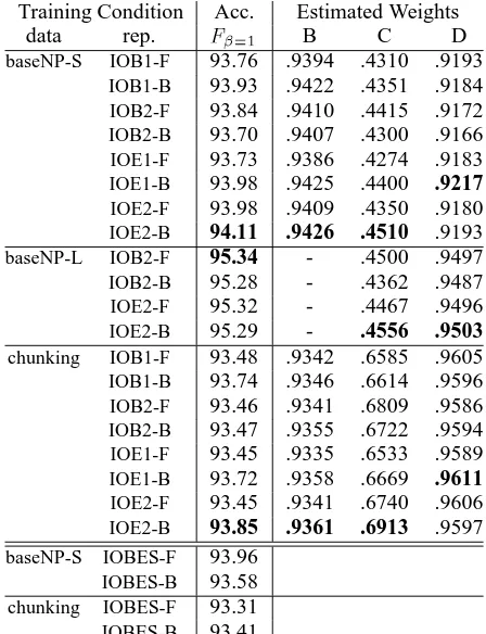
Table 2 shows results of our SVMs based chunk-ing with individual chunk representations. This ta-ble also lists the voting weights estimated by differ-ent approaches (B:Cross Validation, C:VC-bound, D:Leave-one-out). We also show the results of Start/End representation in Table 2.
Table 3 shows the results of the weighted vot-ing of four different votvot-ing methods: A: Uniform, B: Cross Validation (
3µ´
[image:6.612.315.539.72.364.2]), C: VC bound, D: Leave-One-Out Bound.
Table 4 shows the precision, recall and ± ²D³
of the best result for each data set.
4.3 Accuracy vs Chunk Representation
We obtain the best accuracy when we ap-ply IOE2-B representation for baseNP-S and chunking data set. In fact, we cannot find a significant difference in the performance be-tween Inside/Outside(IOB1/IOB2/IOE1/IOE2) and Start/End(IOBES) representations.
Sassano and Utsuro evaluate how the difference of the chunk representation would affect the perfor-mance of the systems based on different machine learning algorithms(Sassano and Utsuro, 2000). They report that Decision List system performs better with Start/End representation than with In-side/Outside, since Decision List considers the spe-cific combination of features. As for Maximum Entropy, they report that it performs better with Inside/Outside representation than with Start/End,
3http://lcg-www.uia.ac.be/conll2000/chunking/ 4
http://cl.aist-nara.ac.jp/ taku-ku/software/TinySVM/
Training Condition Acc. Estimated Weights
data rep. ¶H·¸H¹ B C D
baseNP-S IOB1-F 93.76 .9394 .4310 .9193
IOB1-B 93.93 .9422 .4351 .9184
IOB2-F 93.84 .9410 .4415 .9172
IOB2-B 93.70 .9407 .4300 .9166
IOE1-F 93.73 .9386 .4274 .9183
IOE1-B 93.98 .9425 .4400 .9217
IOE2-F 93.98 .9409 .4350 .9180
IOE2-B 94.11 .9426 .4510 .9193
baseNP-L IOB2-F 95.34 - .4500 .9497
IOB2-B 95.28 - .4362 .9487
IOE2-F 95.32 - .4467 .9496
IOE2-B 95.29 - .4556 .9503
chunking IOB1-F 93.48 .9342 .6585 .9605
IOB1-B 93.74 .9346 .6614 .9596
IOB2-F 93.46 .9341 .6809 .9586
IOB2-B 93.47 .9355 .6722 .9594
IOE1-F 93.45 .9335 .6533 .9589
IOE1-B 93.72 .9358 .6669 .9611
IOE2-F 93.45 .9341 .6740 .9606
IOE2-B 93.85 .9361 .6913 .9597
baseNP-S IOBES-F 93.96 IOBES-B 93.58 chunking IOBES-F 93.31 IOBES-B 93.41
B:Cross Validation, C:VC bound, D:LOO bound
Table 2: Accuracy of individual representations
Training Condition Accuracy¶H·¸H¹
data rep. A B C D
baseNP-S IOB1 94.14 94.20 94.20 94.16
IOB2 94.16 94.22 94.22 94.18 IOE1 94.14 94.19 94.19 94.16 IOE2 94.16 94.20 94.21 94.17
baseNP-L IOB2 95.77 - 95.66 95.66
IOE2 95.77 - 95.66 95.66
chunking IOB1 93.77 93.87 93.89 93.87
IOB2 93.72 93.87 93.90 93.88 IOE1 93.76 93.86 93.88 93.86 IOE2 93.77 93.89 93.91 93.85
A:Uniform Weights, B:Cross Validation C:VC bound, D:LOO bound
Table 3: Results of weighted voting
data set precision recall ± ²D³
baseNP-S 94.15% 94.29% 94.22 baseNP-L 95.62% 95.93% 95.77 chunking 93.89% 93.92% 93.91
[image:6.612.313.542.433.601.2]since Maximum Entropy model regards all features as independent and tries to catch the more general feature sets.
We believe that SVMs perform well regardless of the chunk representation, since SVMs have a high generalization performance and a potential to select the optimal features for the given task.
4.4 Effects of Weighted Voting
By applying weighted voting, we achieve higher ac-curacy than any of single representation system re-gardless of the voting weights. Furthermore, we achieve higher accuracy by applying Cross valida-tion and VC-bound and Leave-One-Out methods than the baseline method.
By using VC bound for each weight, we achieve nearly the same accuracy as that of Cross valida-tion. This result suggests that the VC bound has a potential to predict the error rate for the “true” test data accurately. Focusing on the relationship be-tween the accuracy of the test data and the estimated weights, we find that VC bound can predict the ac-curacy for the test data precisely. Even if we have no room for applying the voting schemes because of some real-world constraints (limited computation and memory capacity), the use of VC bound may al-low to obtain the best accuracy. On the other hand, we find that the prediction ability of Leave-One-Out is worse than that of VC bound.
Cross validation is the standard method to esti-mate the voting weights for different systems. How-ever, Cross validation requires a larger amount of computational overhead as the training data is di-vided and is repeatedly used to obtain the voting weights. We believe that VC bound is more effec-tive than Cross validation, since it can obtain the comparable results to Cross validation without in-creasing computational overhead.
4.5 Comparison with Related Works
Tjong Kim Sang et al. report that they achieve accu-racy of 93.86 for baseNP-S data set, and 94.90 for baseNP-L data set. They apply weighted voting of the systems which are trained using distinct chunk representations and different machine learning al-gorithms such as MBL, ME and IGTree(Tjong Kim Sang, 2000a; Tjong Kim Sang et al., 2000).
Our experiments achieve the accuracy of 93.76 -94.11 for S, and 95.29 - 95.34 for baseNP-L even with a single chunk representation. In addi-tion, by applying the weighted voting framework, we achieve accuracy of 94.22 for baseNP-S, and
95.77 for baseNP-L data set. As far as accuracies
are concerned, our model outperforms Tjong Kim Sang’s model.
In the CoNLL-2000 shared task, we achieved the accuracy of 93.48 using IOB2-F representation (Kudo and Matsumoto, 2000b) 5. By combining weighted voting schemes, we achieve accuracy of
93.91. In addition, our method also outperforms
other methods based on the weighted voting(van Halteren, 2000; Tjong Kim Sang, 2000b).
4.6 Future Work
°
Applying to other chunking tasks
Our chunking method can be equally appli-cable to other chunking task, such as English POS tagging, Japanese chunk(bunsetsu) iden-tification and named entity extraction. For fu-ture, we will apply our method to those chunk-ing tasks and examine the performance of the method.
°
Incorporating variable context length model In our experiments, we simply use the so-called fixed context length model. We believe that we can achieve higher accuracy by select-ing appropriate context length which is actu-ally needed for identifying individual chunk tags. Sassano and Utsuro(Sassano and Ut-suro, 2000) introduce a variable context length model for Japanese named entity identification task and perform better results. We will incor-porate the variable context length model into our system.
°
Considering more predictable bound
In our experiments, we introduce new types of voting methods which stem from the theo-rems of SVMs — VC bound and Leave-One-Out bound. On the other hand, Chapelle and Vapnik introduce an alternative and more pre-dictable bound for the risk and report their proposed bound is quite useful for selecting the kernel function and soft margin parame-ter(Chapelle and Vapnik, 2000). We believe that we can obtain higher accuracy using this more predictable bound for the voting weights in our experiments.
5In our experiments, the accuracy of 93.46 is obtained with
IOB2-F representation, which was the exactly the same repre-sentation we applied for CoNLL 2000 shared task. This slight difference of accuracy arises from the following two reason : (1) The difference of beam width for parsing (N=1 vs. N=5), (2) The difference of applied SVMs package (TinySVM vs.
º`»½¼8¾À¿ÂÁxÃfÄ
5 Summary
In this paper, we introduce a uniform framework for chunking task based on Support Vector Machines (SVMs). Experimental results on WSJ corpus show that our method outperforms other conventional ma-chine learning frameworks such MBL and Max-imum Entropy Models. The results are due to the good characteristics of generalization and non-overfitting of SVMs even with a high dimensional vector space. In addition, we achieve higher accu-racy by applying weighted voting of 8-SVM based systems which are trained using distinct chunk rep-resentations.
References
Erin L. Allwein, Robert E. Schapire, and Yoram Singer. 2000. Reducing multiclass to binary: A unifying approach for margin classifiers. In In-ternational Conf. on Machine Learning (ICML), pages 9–16.
Eric Brill. 1995. Transformation-Based Error-Driven Learning and Natural Language Process-ing: A Case Study in Part-of-Speech Tagging. Computational Linguistics, 21(4).
Oliver Chapelle and Vladimir Vapnik. 2000. Model selection for support vector machines. In Ad-vances in Neural Information Processing Systems 12. Cambridge, Mass: MIT Press.
C. Cortes and Vladimir N. Vapnik. 1995. Support Vector Networks. Machine Learning, 20:273– 297.
T. G. Dietterich and G. Bakiri. 1995. Solving multi-class learning problems via error-correcting out-put codes. Journal of Artificial Intelligence Re-search, 2:263–286.
Yoav Freund and Robert E. Schapire. 1996. Experi-ments with a new boosting algorithm. In Interna-tional Conference on Machine Learning (ICML), pages 148–146.
Thorsten Joachims. 1998. Text Categorization with Support Vector Machines: Learning with Many Relevant Features. In European Conference on Machine Learning (ECML).
Ulrich H.-G Kreßel. 1999. Pairwise Classification and Support Vector Machines. In Advances in Kernel Mathods. MIT Press.
Taku Kudo and Yuji Matsumoto. 2000a. Japanese Dependency Structure Analysis Based on Sup-port Vector Machines. In Empirical Methods in Natural Language Processing and Very Large Corpora, pages 18–25.
Taku Kudo and Yuji Matsumoto. 2000b. Use of Support Vector Learning for Chunk Identifica-tion. In Proceedings of the 4th Conference on CoNLL-2000 and LLL-2000, pages 142–144. Lance A. Ramshaw and Mitchell P. Marcus. 1995.
Text chunking using transformation-based learn-ing. In Proceedings of the 3rd Workshop on Very Large Corpora, pages 88–94.
Manabu Sassano and Takehito Utsuro. 2000. Named Entity Chunking Techniques in Su-pervised Learning for Japanese Named Entity Recognition. In Proceedings of COLING 2000, pages 705–711.
Robert E. Schapire, Yoav Freund, Peter Bartlett, and Wee Sun Lee. 1997. Boosting the margin: a new explanation for the effectiveness of vot-ing methods. In International Conference on Ma-chine Learning (ICML), pages 322–330.
Hirotoshi Taira and Masahiko Haruno. 1999. Fea-ture Selection in SVM Text Categorization. In AAAI-99.
Erik F. Tjong Kim Sang and Sabine Buchholz. 2000. Introduction to the CoNLL-2000 Shared Task: Chunking. In Proceedings of CoNLL-2000 and LLL-2000, pages 127–132.
Erik F. Tjong Kim Sang and Jorn Veenstra. 1999. Representing text chunks. In Proceedings of EACL’99, pages 173–179.
Erik F. Tjong Kim Sang, Walter Daelemans, Herv´e D´ejean, Rob Koeling, Yuval Krymolowski, Vasin Punyakanok, and Dan Roth. 2000. Applying system combination to base noun phrase identi-fication. In Proceedings of COLING 2000, pages 857–863.
Erik F. Tjong Kim Sang. 2000a. Noun phrase recognition by system combination. In Proceed-ings of ANLP-NAACL 2000, pages 50–55. Erik F. Tjong Kim Sang. 2000b. Text Chunking by
System Combination. In Proceedings of CoNLL-2000 and LLL-CoNLL-2000, pages 151–153.
Kiyotaka Uchimoto, Qing Ma, Masaki Murata, Hi-romi Ozaku, and Hitoshi Isahara. 2000. Named Entity Extraction Based on A Maximum Entropy Model and Transformation Rules. In Processing of the ACL 2000.
Hans van Halteren. 2000. Chunking with WPDV Models. In Proceedings of CoNLL-2000 and LLL-2000, pages 154–156.