University of Warwick institutional repository: http://go.warwick.ac.uk/wrap
A Thesis Submitted for the Degree of PhD at the University of Warwick
http://go.warwick.ac.uk/wrap/76651
This thesis is made available online and is protected by original copyright. Please scroll down to view the document itself.
Understanding for Context-Free Point Clouds
Sandro Spina
B.Sc.(Hons), M.Sc.
A thesis submitted in partial fulfilment of the requirements for the degree of
Doctor of Philosophy in Engineering
School of Engineering University of Warwick
List of Publications xi
Acknowledgements xii
Declaration xiii
Abstract xiv
1 Introduction 1
1.1 Structure and Object Identification from Point Clouds . . . 5
1.1.1 Applications . . . 7
1.2 Research Aim . . . 8
1.2.1 PaRSe - Graph-based point cloud segmentation . . . 9
1.2.2 Processing of very large point clouds . . . 10
1.2.3 CoFFrS - Context-free scene understanding framework . . 10
1.3 Thesis Outline . . . 11
2 Preliminaries 12 2.1 Collections . . . 12
2.1.1 Set Comprehensions . . . 12
2.1.2 Set Partitions . . . 13
2.1.3 Power Set and Cartesian Product . . . 14
2.1.4 Relations . . . 14
2.2 Graphs . . . 15
2.2.1 Scene Graph . . . 17
2.2.2 Transition Trees . . . 18
2.2.3 Graph Compatibility . . . 19
2.3 Point Clouds . . . 21
2.3.1 Point Sampling . . . 22
2.3.2 Acquisition Methods . . . 25
2.3.3 Quality . . . 28
2.4 Acceleration Structures for Storing Point Clouds . . . 30
2.4.1 Uniform Grid . . . 31
2.4.2 Kd-tree . . . 31
2.5.2 Principal Component Analysis . . . 32
2.5.3 Volumes . . . 32
2.6 Decimation and Interpolation . . . 34
2.6.1 Point Set Decimation . . . 35
2.6.2 Point Set Up-Sampling . . . 35
2.7 Random Sample Consensus (RanSaC) . . . 36
2.8 Summary . . . 39
3 Segmentation of Point Clouds 40 3.1 Segmentation using Region-Growing Algorithms . . . 42
3.2 Segmentation using Primitive Shape Fitting . . . 46
3.3 Discussion . . . 48
3.4 Summary . . . 50
4 Object Recognition and Indoor Scene Understanding 52 4.1 Object Recognition from Point Clouds . . . 54
4.1.1 Point-Based Object Recognition . . . 57
4.1.2 Segment-Based Object Recognition . . . 67
4.1.3 Summary . . . 72
4.2 Indoor Scene Understanding . . . 73
4.2.1 Supervised Methods . . . 75
4.2.2 Unsupervised Methods . . . 79
4.3 Indoor Scene Understanding Feature Comparison . . . 80
4.4 Discussion . . . 81
4.5 Summary . . . 84
5 Point Cloud Structure Graphs 85 5.1 PaRSe - Method Overview . . . 88
5.1.1 Point Types . . . 90
5.1.2 Segment Types . . . 93
5.2 Generation of Edge and Surface Segments . . . 98
5.2.1 Problems with Surface Generation . . . 101
5.3 RanSaC Plane Fitting . . . 105
5.4 Point Cloud Queries . . . 116
5.5 Results . . . 120
5.5.1 Synthesised point cloud - Kalabsha Temple . . . 120
5.5.2 Cultural Heritage Sites . . . 124
5.5.3 University Green Area . . . 130
5.5.4 Indoor Office Scenes . . . 134
5.5.5 Airborne LiDaR of Maltese Archipelago . . . 136
5.6 Discussion . . . 142
5.6.1 Further Applications . . . 143
5.7 Summary . . . 144
6.1.1 Spatial Subdivision . . . 149
6.1.2 Memory Mapped Files . . . 150
6.2 Concurrent k-NN searches using MMF . . . 150
6.2.1 Loading . . . 152
6.2.2 Sorting . . . 153
6.2.3 Concurrent search for k-NN . . . 156
6.3 Results . . . 157
6.3.1 Execution Time . . . 160
6.4 Discussion . . . 162
6.5 Summary . . . 164
7 Structure Graphs for Indoor Scene Understanding 167 7.1 Method Overview . . . 171
7.1.1 Scanning of Indoor Scenes . . . 174
7.2 Segmentation of Indoor Scenes . . . 174
7.3 Object Graphs . . . 181
7.4 Scene Understanding . . . 187
7.5 Results . . . 200
7.5.1 Indoor Scenes from Nan et al. (2012) . . . 203
7.5.2 Additional Indoor Scenes . . . 210
7.6 Discussion . . . 217
7.7 Summary . . . 220
8 Conclusions and Future Work 221 8.1 Contributions . . . 221
8.1.1 Plane-fitting and region-growing Segmentation (PaRSe) . . 222
8.1.2 Fast Scalable Out-of-Core k-NN Searches . . . 223
8.1.3 Context-Free Framework for Scene Understanding (CoFFrS) 224 8.2 Synopsis . . . 225
8.3 Impact . . . 227
8.4 Limitations and Future Work . . . 229
8.5 Final Remarks . . . 231
References 231
1.1 Acquisition of a scene . . . 2
1.2 Semantic interpretation of a scene . . . 3
1.3 Challenges in scene understanding from point clouds . . . 5
1.4 Examples of point cloud data sets . . . 6
1.5 A general purpose point cloud processing pipeline . . . 9
2.1 Four valid set partitions of the set {1,2,3,4,5,6,7,8,9} . . . 14
2.2 Arrows describing a relation between objects . . . 15
2.3 Graphs describing different problems . . . 16
2.4 Scene graph of a 2D scene . . . 18
2.5 Transition trees examples . . . 19
2.6 2D shapes with their respective graphs . . . 20
2.7 Graph compatibility using transition trees . . . 21
2.8 Sampling of cylinder primitive shape . . . 22
2.9 The function x traces a surface patch in R3 . . . . 23
2.10 Sampling as a ray casting process . . . 24
2.11 Sampling using triangulation-based scanners . . . 26
2.12 Point clouds acquired using commodity scanners . . . 27
2.13 Sampling densities according to distance from object . . . 27
2.14 Point clouds acquired using time-of-flight scanners . . . 29
2.15 Set of points partitioned using a uniform grid . . . 31
2.16 Points partitioned into two lines and one circle . . . 37
2.17 Randomness in the choice of supports in RanSaC . . . 38
3.1 Ambiguity in point cloud segmentation algorithms . . . 41
3.2 Segmentation determines primitives used to identify objects . . . 42
4.1 A 2D scene understanding process . . . 53
4.2 Approaches to shape recognition and scene understanding . . . . 55
4.5 Example of a spin-images descriptor . . . 59
4.6 Example of surface signature descriptor . . . 61
4.7 3D shape descriptor using histogram bins . . . 62
4.8 Example of point feature histogram descriptor . . . 65
5.1 Segmentation pipeline applied to pre-historic wall structure . . . . 85
5.2 Mnajdra pre-historic temple point cloud . . . 87
5.3 Levels of abstraction over a point cloudP . . . 89
5.4 Point cloud of line segments . . . 91
5.5 Point tagging withkmax=3, α=2 and variable point density . . . . 94
5.6 Point tagging withα=2 andkmax=5,7,9 . . . 95
5.7 Edge points from 4 primitive objects . . . 96
5.8 Points sampled from the surface of a turtle . . . 96
5.9 Examples of edge and surface points . . . 97
5.10 Obelisk segmentation process into edge and surface segments . . . 98
5.11 Non-symmetry of neighbourhood membership . . . 100
5.12 State merging in structure graph . . . 101
5.13 Under and over segmentation . . . 103
5.14 Panorama photograph of temple apse . . . 104
5.15 Details of temple apse and over-segmentation . . . 106
5.16 Segmentation of synthesised conference room . . . 107
5.17 Structure graph of Cornell box point cloud . . . 108
5.18 Plane parameters for RanSaC fitting . . . 111
5.19 Plane primitives fitted to obelisk segments . . . 112
5.20 Connectivity between ∗·planar segments in box graph . . . 114
5.21 Example of connectivity between stairs segments . . . 115
5.22 Query graph describing a cylinder using geometric constrains . . . 117
5.23 Query graph using seed segments . . . 118
5.24 Point clouds of the synthesised Kalabsha temple . . . 121
5.25 Column extraction from Kalabsha temple point cloud . . . 122
5.26 Point labelling and surface·planar segments of Mnajdra . . . 123
5.27 Application of query graphs on Mnajdra temple . . . 125
5.28 Largest surf ace and edge segments . . . 126
5.29 Hal-Tarxien point cloud after region-growing and RanSaC fitting . 127 5.30 Hal-Tarxien surface and edge segments . . . 128
5.33 Segmentation of church at Lans le Villard . . . 131
5.34 Roof details, slabs, extracted from segmentation process . . . 132
5.35 Tombstones and window details of the Lans le Villard church . . . 133
5.36 Over segmentation in areas of the Lans le Villard . . . 133
5.37 Query graph used to extract trees from park . . . 134
5.38 Application of trees query graph . . . 135
5.39 Extraction of desktop items from office scene . . . 137
5.40 Segments representing specific objects in point cloud . . . 138
5.41 Segment representing main road network . . . 139
5.42 Segments representing fields in a LiDaR point cloud . . . 139
5.43 Extraction of desk lamp and on shelve items from office scene . . 140
5.44 Segmentation results for a LiDaR data set . . . 141
6.1 Songo Mnara point cloud consisting of 45M points . . . 148
6.2 Input point cloud is loaded in segments. . . 152
6.3 Sparse grid decomposition and cell ordering . . . 154
6.4 Ghost cells and points . . . 156
6.5 The three point clouds used in the results . . . 165
6.6 Optional caption for list of figures . . . 166
7.1 Photographs of typical indoor environments . . . 168
7.2 CoFFrS pipeline components from raw point cloud . . . 169
7.3 Scene Segmentation and Understanding Pipeline Overview . . . . 173
7.4 Example point clouds of indoor scenes . . . 175
7.5 Close up on table and three chairs of office room . . . 176
7.6 Segmentation process on two chairs and an office . . . 177
7.7 Over segmentation in scene from Nan et al. (2012) . . . 178
7.8 RanSaC plane fitting on region grown segment . . . 178
7.9 Description and example of segment spatial context . . . 179
7.10 Coverage score computed on OBB around segment . . . 180
7.11 Point cloud from Nan et al. (2012) - five chairs with different poses 181 7.12 Chair 3D model is scanned and segmented . . . 183
7.13 Connectivity between anchor segments . . . 184
7.14 Three depth images from virtual camera around an object . . . . 187
7.15 A simple Markov decision process tree . . . 188
7.16 2D grid computed around the anchor segment . . . 194
7.19 2D representation of voxel grids around anchors . . . 200
7.20 Definition of boundaries query graph . . . 201
7.21 Definition of shelving query graph . . . 202
7.22 Definition of stairs query graph . . . 203
7.23 Subset of point clouds used by Nan et al. (2012) . . . 203
7.24 All chairs are matched to the chair object graph . . . 204
7.25 Scene understanding result for room with couches . . . 205
7.26 Scene understanding result for office room . . . 205
7.27 Examples showing details produced by PaRSe . . . 206
7.28 Extraction of boundary and anchor segments . . . 206
7.29 Over-segmentation producing many edge segments . . . 207
7.30 Point cloud of trained round table-top table . . . 208
7.31 Inclusion and matching of round table object graph . . . 208
7.32 Matching grids overlaid in indoor scene . . . 209
7.33 Table or cabinet ambiguity in matching process . . . 210
7.34 A low density point cloud acquired using the Asus Xtion sensor . 210 7.35 Plane fitting on couch segment matches couch object graph anchors211 7.36 Scene understanding process for office with chairs and shelving unit214 7.37 Shelving cabinet cluttered with files, boxes and books . . . 215
7.38 Scene understanding process for office with tilted chairs and occlusion215 7.39 CoFFrS applied on office with multiple shelving cabinets . . . 216
7.40 CoFFrS applied on scene with steps . . . 216
7.41 Lack of supporting segments to identify chairs . . . 218
2.1 Set partitions computed according to angle values . . . 20
3.1 Summary of point cloud segmentation techniques . . . 51
4.1 Summary of object/structure recognition techniques using point-based descriptors. . . 73
4.2 Summary of object/structure recognition techniques based on seg-mentation. . . 73
4.3 Summary of techniques used for specific object recognition tasks. 74 4.4 Comparison of scene understanding methods . . . 82
5.1 Segmentation parameters used in results section . . . 119
6.1 Point clouds, corresponding number of points and number of cells created during loading phase in sparse grid . . . 159
6.2 Execution times (in seconds) using 8GB RAM . . . 160
6.3 Execution times (in seconds) using 4GB RAM . . . 162
6.4 Execution times (in seconds) using 2GB RAM . . . 162
6.5 Execution times (in seconds) using 1GB RAM . . . 163
6.6 Varying values of M on the songoX2 data set (with 1GB RAM installed) . . . 163
8.1 Comparison of indoor scene understanding methods . . . 228
Papers
Spina, S., Debattista, K., Bugeja, K. & Chalmers, A. (2011). Point cloud
segmentation for cultural heritage sites, 12th International conference on Virtual Reality, Archaeology and Cultural Heritage, The Eurographics As-sociation, pp. 41-48.
Spina, S., Debattista, K., Bugeja, K. & Chalmers, A. (2012). Fast
scal-able k-NN computation for very large point clouds, Theory and Practice of Computer Graphics, The Eurographics Association, pp. 85-92.
Spina, S., Debattista, K., Bugeja, K. & Chalmers, A. (2014). Scene
semg-mentation and understanding for context-free point clouds, Pacific Confer-ence on Computer Graphics and Applications - Short Papers, The Euro-graphics Association, pp. 7-12.
Publications under preparation
PaRSe - A graph-based segmentation method for raw generic point clouds (Chapter 5, extended), for Computer Graphics and Application
I would first like to express my appreciation and gratitude to my advisors Kurt and Alan;
without your guidance, motivation and continuous support this thesis would not have been
possible. Many thanks for the opportunities given and for always encouraging my research.
Thanks also go to those in the Visualisation Group. Special thanks to Kurt, Vedad, Belma
and Elmedin who have tremendously helped me during my many research visits by always
welcoming me in their homes.
I would also like to thank my colleagues at the Department of Computer Science. In
particu-lar, Keith and Kevin, for voluntarily taking my teaching load during this final year, and thus
allowing me to keep focused on this thesis.
Keith, your input has massively contributed to raising the quality of this work. My heartfelt
thanks!
My most profound gratitude goes to all my family, especially my parents Rita and Frans, my
brother Claudio, various uncles and aunties, for always being there and supporting me
through-out.
Finally, and most importantly, I would like to thank my beloved wife and daughters. Stefania,
without your patience and support this thesis would not have been possible. Eliana and Clara,
you were a continuous source of energy; thanks for filling my sails when the ship was at a
standstill.
The work in this thesis is original and no portion of this work has been submitted
in support of an application for another degree or qualification at this university
or at another university or institution of learning.
Sandro Spina
The acquisition of 3D point clouds representing the surface structure of real-world
scenes has become common practice in many areas including architecture,
cul-tural heritage and urban planning. Improvements in sample acquisition rates and precision are contributing to an increase in size and quality of point cloud data.
The management of these large volumes of data is quickly becoming a challenge,
leading to the design of algorithms intended to analyse and decrease the
com-plexity of this data. Point cloud segmentation algorithms partition point clouds
for better management, and scene understanding algorithms identify the
compo-nents of a scene in the presence of considerable clutter and noise. In many cases,
segmentation algorithms operate within the remit of a specific context, wherein
their effectiveness is measured. Similarly, scene understanding algorithms depend
on specific scene properties and fail to identify objects in a number of situations. This work addresses this lack of generality in current segmentation and scene
understanding processes, and proposes methods for point clouds acquired using
diverse scanning technologies in a wide spectrum of contexts. The approach to
segmentation proposed by this work partitions a point cloud with minimal
infor-mation, abstracting the data into a set of connected segment primitives to support
efficient manipulation. A graph-based query mechanism is used to express further
relations between segments and provide the building blocks for scene
understand-ing. The presented method for scene understanding is agnostic of scene-specific
context and supports both supervised and unsupervised approaches. In the for-mer, a graph-based object descriptor is derived from a training process and used
in object identification. The latter approach applies pattern matching to identify
regular structures. A novel external memory algorithm based on a hybrid spatial
subdivision technique is introduced to handle very large point clouds and
acceler-ate the computation of the k-nearest neighbour function. Segmentation has been
ing has been successfully applied to indoor scenes on which other methods fail. The overall results demonstrate that the context-agnostic methods presented in
this work can be successfully employed to manage the complexity of ever growing
repositories.
Keywords: computer graphics, point cloud processing, segmentation, scene un-derstanding, object tagging
Introduction
Over the past decade, digital photography has been adopted by a large segment
of the population with digital cameras becoming less expensive, more advanced
and ubiquitous. This has led to the creation of massive repositories of digital
content in the form of images and videos. To address this continuous increase
in content, research has looked into ways of automatically organising this data
by using information contained within these images. In particular, computer vision and image processing techniques have been designed to reason about the
content in this data. For instance, face recognition algorithms have experienced
rapid advances and are now employed on social networks and digital cameras to
associate people to photos in which they are visible. The application of these
algorithms adds semantic layers to digital content, which otherwise would simply
consist of a set of coloured pixels when processed by a computer system.
More recently, another digital representation is growing in popularity, one
that describes the geometric surface structure of real-world objects. Instead of
using colour sensors to capture the appearance, 3D cameras or scanners use depth sensors to measure the distance to the objects in view and produce a set
of points in space, a point cloud. Both images and point clouds are necessary
to capture different aspects of a scene. In a similar fashion to digital cameras,
continuous improvements in 3D scanning technologies resulting in improved
pre-cision and higher acquisition rates, have been contributing towards an increase in
the creation and size of point cloud content. This growth is accentuated by the
widespread popularity of commodity hardware which is primarily intended for
the acquisition of small indoor environments. As a result, applications making
use of point clouds have increased, with the acquisition of 3D point information becoming common practice in many areas including architecture, cultural
Sunflower
Image Processing
Acquisition using Depth Sensing Hardware
Acquisition using Photogrammetry
Post Processing (Segmentation)
3D Object Recognition
[image:18.595.119.516.98.246.2]Box
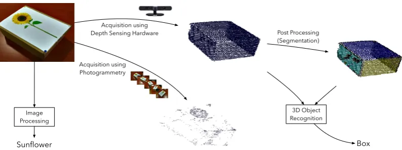
Figure 1.1: Acquisition of a scene into a digital representation, either as a 2D image or 3D point cloud. In the latter case, different methods can be used to scan the scene resulting in different results. The identification of objects in the scene depends on the digital representation and algorithms used. Segmentation plays an important part in the recognition process.
itage (CH), manufacturing and urban planning. A common underlying problem faced within these different domains is the increased complexity in handling these
large data sets, typically ranging from a few thousand to several million points,
which has resulted in the need for automated mechanisms to organise and hence
facilitate the manipulation of point clouds.
While it may be a trivial task for a person to recognise objects and structures
in an image or a point cloud, this is not a straightforward task for a computer
sys-tem. This is particularly challenging in scenes comprised of an unknown number
of different objects, where the complexity of the identification task is augmented
with the added challenge of determining object boundaries, with objects which may only be partially visible to the sensor due to inter-object occlusions.
Typi-cally, using both appearance and shape information increases the potential for a
correct interpretation of a scene. Figure 1.1 illustrates an example, where image
processing techniques may correctly identify a sunflower and 3D object
recogni-tion techniques may determine the presence of a box. The combinarecogni-tion of these
results may contribute to a better interpretation of the scene, such that the
com-puter system can now deduce that the scene contains a box with a sunflower
picture on one of its sides. In many cases, however, information related to the
appearance of a scene is not available with point clouds. For instance, in many point clouds used as case studies in this thesis the acquisition process is carried
out by third parties, and only position information per point is made available.
coordi-Image Processing Techniques
Object Recognition Techniques
+
Scene Understanding Techniques
Digital Scene Representation
{ Circle, Diamond, Triangle, Star }
{Blue, Yellow, Red }
{Blue Diamond, Blue Star, Yellow Triangle, Red Circle}
Figure 1.2: Given a digital representation of a scene, image processing, object recogni-tion and scene understanding techniques have been used to identify the entities/objects contained in the scene. The output is an association between elements of the digital representation and a semantic interpretation, in this case for coloured shapes.
nate space to create a higher quality point cloud, with each depth sensor view
contributing surface points which may not be visible from the other views. In
particular, Iterative Closest Point (ICP) algorithms are used to combine
individ-ual scanner views into one consistent point cloud, and Simultaneous Localization
and Mapping (SLAM) techniques are used to construct a point cloud of a scene by
continuously keeping track of the scanner’s location within the scene. Figure 1.1
illustrates the application of these techniques to produce a point cloud which
closely matches the shape of the box in the image using depth sensing hardware.
Following acquisition, a segmentation process can optionally be applied to parti-tion the point cloud into groups of related points, where in this case, the groups,
rendered using different colours, represent the four sampled sides of the box.
This additional information may be used by a 3D object recognition algorithm
to deduce that the point cloud represents a box. Analogous to a programming
language compiler front-end, segmentation may be viewed as the tokenizer (or
lexer) of the input stream, whereas 3D object recognition may be viewed as the
parser, which groups together tokens representing specific constructs in the
lan-guage. In the case of point clouds, these groups of points, referred to as segments,
may be subsequently used to carry out a variety of tasks, for instance removing objects from a scene to improve visualisation, or measuring distances between
the boundaries of a room.
from point clouds, which include 3D object recognition and scene understanding
techniques. In both cases, the result consists of a mapping between point subsets
of the scene point cloud and semantic labels. Scene understanding algorithms have traditionally been employed to classify images of scenes into semantic
cate-gories; for instance, an input data set classified as an office space. The many
dif-ferent techniques can be divided into two main categories, namely scene-centred
approaches and object-centred approaches. In the former, characteristics of the
scene such as clutter and symmetry are used for classification, whereas in the
lat-ter, classification depends on the identification of objects such as plants, chairs
and tables. These algorithms find application in numerous fields by contributing
additional semantic information, particularly when the input is a set of images,
but also when the input is a point cloud. Figure 1.3 illustrates a point cloud
of a typical scene acquired using triangulation-based (§2.3.2) depth sensors. An autonomous navigation unit moving around such an environment would certainly
benefit from the understanding of surrounding structures, for instance, if given
the task of locating an object on a shelve or a table. In these scenarios, the
majority of samples are initially taken from the surfaces of the larger objects
in the scene, such as the table, chairs and shelving. Since fewer samples cover
small objects that lie on the table or the floor, identification of these elements
becomes more challenging. Proper identification of these smaller objects requires
a separate acquisition step which only considers a small portion of the room such
as the table top, or shelve. If an autonomous navigation system can properly interpret the room, then it can focus its scanners on the smaller section of the
room to locate the required object. 3D object recognition techniques (§4.1) have predominantly been used to identify these small objects using a myriad of
point-based object descriptors. On the other hand, scene understanding techniques
(§4.2) have been employed to identify the more prominent components of a scene by making use of segment-based scene descriptors, which encode via a training
process the objects making up a scene. This approach has been shown to be very
sensitive to changes in the object’s poses between trained and unseen scenes. For
instance, toppled or inclined chairs similar to those in the office point cloud of Figure 1.3 are not correctly classified by any of the state of the art indoor scene
understanding techniques. The chair on a table example highlights another
short-coming of these techniques, in that many work on the assumption that objects
are always located at pre-established distances from a user-defined ground. The
Toppled chair on the floor
Shelving units
Table Inclined chair
Chair
Chair on a table
Room floor Something on the floor
Figure 1.3: Scene understanding of indoor scenes from point clouds acquired using com-modity triangulation-based hardware are typically noisy and cluttered. Moreover these may contain static objects in different poses (chairs) and varying structures (shelving). In order to cover the entire room, the point cloud resolution is not sufficient to identify small objects (object on the floor and shelving units).
1.1
Structure and Object Identification from Point Clouds
Figure 1.4 illustrates point clouds scanned using a variety of scanning
technolo-gies. These include long-range time-of-flight laser scanners to acquire the
Mna-jdra and Tarxien pre-historic sites over a number of hours (second row), and
commodity hardware such as the triangulation-based Asus Xtion scanner, to
ac-quire the office scene in under 1 minute (first row). Segmentation algorithms
(Chapter 3) are necessary when working on very large point clouds, for tasks
such as visualisation, editing and storage. In some cases, segmentation can be as
straightforward as partitioning the points into equally sized regions, as shown in Figure 1.4 (bottom row). Other more complex tasks, such as object recognition or
distance measurements, require the use of a more elaborate segmentation process,
where the output segments correspond to some meaningful concept. For instance,
in the case of object recognition, segments could represent tables and chairs, and
in the case of distance measurements, segments could represent structures such
as floors, walls and ceilings. General purpose segmentation adopts two principal
approaches, namely using processes that fit primitive geometric shapes, such as
spheres and cylinders, to the input point cloud, and region-growing processes
which expand segments from seed points by following some surface property cri-teria such as curvature. Both approaches make a number of assumptions about
tive shapes used, and in the second, that the points are sampled from a relatively
smooth surface with minimal sensor noise. Within these two approaches,
pro-cesses have been tailored to suit specific scenarios, for instance segmentation of point clouds representing buildings, trees or industrial objects. The
identifica-tion of objects and scene structures such as the floor, stairs or shelving, heavily
depends on the segments produced. Whereas segmentation algorithms group
points into related clusters, they do not provide a semantic interpretation for the
segments. Instead, the grouping and labelling of these segments is the remit of
scene understanding and object recognition algorithms. For instance, a number
of segments corresponding to the steps of a flight of stairs, are grouped together
and labelled appropriately as stairs. In addition to correct segmentation results,
many indoor scene understanding methods also rely on scene-specific parameters;
for example, the upward direction of the scene and distances between an object and the ground. This leads to scenarios where slightly changing the size, pose,
or vertical position of an object (e.g. Figure 1.3) renders the method ineffective.
1.1.1
Applications
Many tasks carried out in a variety of fields can benefit from segmentation, 3D
object recognition and scene understanding methods from point clouds.
Cultural Heritage
Many institutions are engaged in the acquisition of point clouds
repre-senting sites and objects of significant CH importance. Segmentation is
necessary for documentation and preservation of a site or object, and
en-ables realistic virtual reconstructions and dissemination to the general
pub-lic (Yastikli, 2007; Rinaudoet al., 2010).
Architecture
Semantically rich digital facility models are usually produced from
com-puter aided design (CAD) models of a building. Given the variance
be-tween CAD models and what is actually built, indoor scene
understand-ing techniques have recently emerged which use point clouds acquired
us-ing laser scanners to automatically synthesise buildus-ing information models
(BIM) (Tang et al., 2010).
Planning
with data acquired using a variety of sensors and acquisition techniques.
In particular, airborne LiDaR scanners producing accurate terrain 3D
in-formation greatly simplifies large-scale urban modelling (Hu et al., 2003). Segmentation and object recognition techniques have been used to
acceler-ate the post-processing effort by automatically partitioning the data into
urban entities.
Robotics
Autonomous robot localisation and navigation greatly benefits from the availability of sensors capable of capturing depth information, for instance
to prevent collisions and to locate specific objects (Biswas & Veloso, 2012).
Indoor scene understanding techniques allow these autonomous robots the
possibility of reasoning about their surroundings.
Manufacturing
Advances in 3D printing technologies have brought about a paradigm shift
in the manufacturing process of small objects. Scanning technologies are
used in order to manufacture replicas of real-world objects, which can then
be accordingly modified using appropriate segmentation algorithms and 3D
printed (Lipson & Kurman, 2013).
1.2
Research Aim
The research aim of this thesis is the advancement of techniques intended to
facilitate the reasoning about and management of point clouds. Both
segmen-tation and scene understanding methods contribute towards this goal. Previous
indoor scene understanding methods, using both supervised and unsupervised
approaches, have shown merit in reasoning about indoor scenes, but have so far
depended on scene-specific context in their interpretation process. This thesis
looks into filling this gap by designing a context-free scene understanding frame-work which is able to, without using scene-specific parameters, provide a valid
interpretation for scenes such as the office in Figure 1.3. Segmentation is a critical
component of this pipeline. Therefore, this work also looks at the development of
a general purpose segmentation algorithm, which is able to reliably partition low
quality point clouds acquired using commodity depth sensors for indoor scene
understanding purposes, but which is also suited to partition point clouds
Physical Scene Sampling
Segmentation Methods Unstructured Points
Structure
Point cloud processing algorithms
chair robot roof
Segmentation Primitives Data Interpretation / Objects
Figure 1.5: Rather than producing multiple point cloud processing pipelines where segmentation and task related processing methods are purposely designed to fit specific tasks, a context-free point cloud processing pipeline tries to minimise the set up required to address tasks from a variety of domains.
1.5). For this purpose, this thesis looks into the design of a general-purpose point
cloud segmentation process which combines the advantages of both shape fitting and region-growing approaches.
1.2.1
PaRSe - Graph-based point cloud segmentation
For most tasks, manipulation of a point cloud usually requires extensive expertise
in the use of CAD and modelling software. In this work, automated mechanisms
which alleviate some of these tasks are presented in the form of a graph-based
point cloud segmentation process, referred to as PaRSe, which combines the
benefits of region-growing and primitive fitting approaches. Rather than just
partitioning the input into a list of segments, a structure graph is built during the
segmentation process which describes connectivity information between segment
primitives. A variety of point clouds are used to evaluate the generality of the
approach in supporting different tasks.
Objectives
• to design a general purpose segmentation algorithm
1.2.2
Processing of very large point clouds
In some cases, the size of the point cloud acquired is so large that it does not
entirely fit in main memory. The majority of post-processing algorithms, such
as segmentation, work under the assumption that the data sets operated on can
fit in main memory, while others take into account the size of the data sets and
are thus designed to keep data on disk. For many post-processing algorithms, a
considerable amount of time is spent searching for the k-nearest neighbour (k-NN)
of each point. Optimal performance results are achieved when k-NN computation
is carried out in-core, i.e. when both points and acceleration structure are stored in main memory. On the other hand out-of-core techniques take into account the
size of the points but are much slower due to overheads related to disk I/O. A
novel out-of-core algorithm is presented in this thesis, which maximizes processor
utilization while keeping I/O overheads to a minimum.
Objectives
• to enable the execution of point cloud segmentation on devices with limited memory
• to design an out-of-core k-NN process with similar running times to an in-memory approach
1.2.3
CoFFrS - Context-free scene understanding framework
The method to scene understanding presented in this thesis adopts a supervised
approach. However, rather than using a training set of scenes to synthesise a
scene descriptor and thus limiting its applicability to very similar unseen scenes,
individual descriptors representing generic objects in the scene are synthesised
us-ing PaRSe and the inclusion of additional shape-related information. Searches for
specific segment patterns in the input point cloud are used to recognise structures such as room boundaries and shelving. A novel scene understanding framework
is introduced, referred to as CoFFrS, which first identifies scene structures by
searching for specific segment patterns and then associates the remaining
Objectives
• to design a scene understanding method that is not sensitive to changes in object pose and scene parameters
• to determine, using a qualitative approach, its effectiveness against scenes from previous literature and new ones
1.3
Thesis Outline
This thesis is organised as follows:
Chapter 2: Preliminaries provides a comprehensive overview of concepts, def-initions and notation used throughout the rest of the thesis.
Chapter 3: Segmentation of Point Clouds provides a detailed literature re-view of the various segmentation methods used on point clouds.
Chapter 4: Object Recognition and Indoor Scene Understanding
provides a detailed literature review on the methods used for 3D object
recognition and indoor scene understanding from point clouds.
Chapter 5: Point Cloud Structure Graphs presents a general purpose graph-based segmentation algorithm and outlines its utility in a variety of tasks.
Chapter 6: Fast Scalable k-NN Searches for Very Large Point Clouds
presents a novel out-of-core algorithm which enables devices with limited
memory to carry out point cloud segmentation processes.
Chapter 7: Structure Graphs for Indoor Scene Understanding presents a novel pipeline for scene understanding tasks which does not rely on a
spe-cific scene context.
Chapter 8: Conclusions concludes the dissertation, discussing contributions and limitations of this work and presenting potential avenues for future
Preliminaries
This chapter provides a comprehensive overview of concepts, definitions and
no-tation used throughout the rest of the thesis. The nono-tation used for sets and
operations on them is first defined, followed by a description of point clouds
in terms of this notation, together with a number of properties and operations
generally associated with them. The acceleration structures used to speed-up
computations on point clouds are then briefly outlined, followed by a description of a number of operations on points which take advantage of these acceleration
structures.
2.1
Collections
An important concept in mathematics and computer science is that of a
col-lection of objects with similar type. Within these colcol-lections, both order and
repetition may or may not be important. In this section sets are defined, which are collections in which neither order nor repetition is important.
2.1.1
Set Comprehensions
The simplest way to define a set is by listing all elements in the collection. For
example, the set of days in the week D = {M onday, T uesday, W ednesday, T hursday, F riday, Saturday, Sunday}. One important set is the one which contains no elements, the empty set: ∅. In general, it is useful to define sets in terms of properties that their elements are expected to satisfy, with properties
expressed as predicates. Consider for example, the set of nationalities of football players who scored at least once in a world cup competition. The notation used
to define sets in terms of properties is called set comprehension and is used to construct sets without having to list all elements:
{p:P erson|p∈W orldCupF ootballers∧score(p)≥1•nationalityOf(p)}
The symbols | and • separate the three parts of the set comprehension. The first part, declaration, declares the variables used in the definition, the second part is a predicate and the third part, theterm, gives an expression representing the objects inserted in the new set. If instead of the nationalities of the players,
age of each player which satisfies the predicate needs to be constructed, then the
term can be changed to ageOf(p). Both predicate and term can sometimes be omitted. For example, the term in the previous comprehension can be dropped
to return persons. Moreover, if there are no constraints in the predicate part, i.e. this always evaluates to true, the predicate part can be omitted.
More complex properties on sets can be described using predicate
quantifi-cation. These include universal quantification (∀) and existential quantification (∃) which are used to state that all or at least one objects in a set satisfy a particular property. Set operators such as subset (S ⊆ T), equality (S == T), union (S∪T), intersection (S∩T), and difference (S\T) provide a mechanism for comparing sets and for creating new ones using sets which are already
de-fined. Union and intersection operators can be generalised in order for them to
be applied on a number of sets rather than just two.
2.1.2
Set Partitions
Generalised union enables the introduction of the notion of a partition of a set. For instance, given the set of all players participating in the world cup, one
possible set partition is the one which creates 32 sets, with each set representing
a specific team. Team membership is said to partition the set of players since (i)
all players must be in at least one team, and (ii) players may not be in more than
one of the teams. Each partition is a subset of the original set and is defined as
follows:
Definition Given an index set I and sets Pi for every i ∈ I, we say that the
indexed sets partition a set S if (i) they include all elements ofS, i. e. S
i∈IPi =
S; and (ii) any two different partitions Pi and Pj have no common elements:
2 1 4 3 8 7 5 6 9 2 1 4 3 8 7 5 6 9 2 1 4 3 8 7 5 6 9 2 1 4 3 8 7 5 6 9
{{1,2,3},{4},{5,6,7,8,9}} {{1,2,3,4,5,6,7,8},{9}} {{1},{2,4},{3,5},{6,7,8},{9}} {{1},{2},{4},{3},{5},{6},{7},{9},{8}}
Figure 2.1: Four valid set partitions of the set{1,2,3,4,5,6,7,8,9}
Given the set {1,2,3,4,5,6,7,8,9}, Figure 2.1 shows a sample of valid set par-titions. Set partitions provide a mechanism to cluster objects within a set, with
the elements of the partition themselves sets, which can be modified using the
set operators described above.
2.1.3
Power Set and Cartesian Product
The elements of a set partition of S are all subsets of S. The power set of
S, written P(S), gives an enumeration of all these possible subsets. Using set comprehension, the power set is constructed as follows:
Definition Given a set S containing objects of type X, the power set of S, written as P(S), is defined to be the set of all subsets of S:
P(S)def= {T|T ⊆S}
Given a set S containingn objects, P(S) contains 2n objects. The Cartesian Product between sets provides a mechanism to combine objects from distinct sets. Using set comprehension, the Cartesian Product between two sets is defined as
follows:
Definition Given a set S of type X, and another T of type Y, the Cartesian Product of S and T, written as S×T, is defines to be the set of all pairs with the first object an element of S, and second object an element of T:
S×T def={x:X, y :Y|x∈S∧y∈T •(x, y)}
2.1.4
Relations
The notation and operations defined so far are used to construct and manipulate
{1,2}
{4,6,8,12}
{3,5}
{9} {10,11}
h
a
s
C
o
l
o
u
r
Figure 2.2: Arrows describe a relation between objects. In this case between objects in a set partition and colours in another set.
between these objects. Given setsS and T, a relation between these sets can be created to map in some specific way objects from one set to the other. Whereas
the Cartesian Product denotes the upper bound on the number of mappings
pos-sible between objects in sets, a relation is used to define specific correspondences
between these objects. Figure 2.2 illustrates two sets storing objects of different
type. The set on the left shows a specific set partition, whereas the one on the right contains three objects, namely colours red, green and blue. A relation, for instance hasColour represented as arrows, maps objects from one set to the other. Note that not all objects need to form part of this mapping. For instance,
in the case of object {10,11}, the relation hasColour is undef ined. Relations can naturally be expressed as sets of pairs. The use of sets to express relations
enables the use of set comprehension to construct relations and the set operators
previously defined can be used to combine relations of the same type.
2.2
Graphs
Figure 2.3 illustrates two graphs representing two different problems. In the first
(left) nodes represent towns, whereas in the second (right) nodes represent process
state. Despite representing different problems, they exhibit common features, in
that both consist of a number of nodes (vertices or states) connected via arcs
(edges or transitions) and both nodes and arcs carry some relevant information.
Marsa Zurrieq Safi Hamrun Sliema 5M 4M 10Miles 3M 2M 12Miles 6M 1.5M running ready blocked done new run create I/O finish time exp’d termination I/O req
Figure 2.3: Graphs representing two different problems. In the first distances between towns is shown, whereas the second describes transitions between the different states of a running process.
which describes the different running process state transitions, or else undirected
as in the distances between towns example. For the towns distance graph, this
relation can be used to answer queries such as give me three towns whose total distance between them is less than 6 miles. The labelled arcs provide sufficient information such that the set {Zurrieq, Sliema, Hamrun} can be computed. In the case of the running process graph, the relation can answer queries such asis create, run and termination a valid sequence of events? which is clearly valid and returns the set{new, ready, running, done}enumerating the nodes visited whilst moving through the sequence. Arcs in the graph can be represented as triples (v, l, v0), wherev and v0 denote nodes in the graph connected via the labelled arc
l. A graph is defined as follows:
Definition The graph G= (V, L, E), consists of a set of nodesV, a set of labels
L, and a set of labelled arcs between vertices E ⊆V ×L×V.
Labels can be used as predicates and thus enable a more generic method of
attaching semantics to arcs and nodes. Consider for example augmenting the
labels of the towns distances graph with elevation information in addition to
distance. Arcs of the form (v, l, v0) are extended to (v, < l, m >, v0), such that (M arsa,6M, Saf i) becomes (M arsa, < 6M,200m >, Saf i) by extending labels to vectors of information. A similar approach is taken with node labels, for
instance instead of including elevation information in E, elevation values can be included within nodes in addition of town names. In general, graph labels for
both nodes and arcs take the form of a sequence of key, value pairs. Keys are
unique whereas values depend on what property is being modelled. In the case of
town names, values can simply be a string of characters; in the case of elevation,
from a pre-established set of possibilities. For instance, if the exact population
size is not important in terms of numbers,sizevalues can be selected from the set
{small, medium, large}. Rather than placing queries on a graphG={V, L, E}, of the type What is the distance betweenZurrieq andSaf i?, it is sometimes useful to query the graph with Are there two towns whose distance between them is less that 4 miles?. The answer to this query is the set of pairs of nodes which satisfy the predicate, in this case {(Zurrieq, Sliema),(Zurrieq, Hamrun)}. Using set comprehension notation, and assuming adistancefunction is available, this query is expressed as follows:
{(v, l, v0) :E|distance(l)<4•(nameOf(v), nameOf(v0))}
2.2.1
Scene Graph
Graphs may be used to represent many different concepts. One which is closely
related to computer graphics, is the scene graph, which in its basic form models the spatial relationships between objects in a virtual scene. Figure 2.4 illustrates
a 2D scene of a room and a scene graph describing it. In its basic form, the
scene graph is used to group together similar objects. For instance, furniture
objects including tables and chairs are all located under the nodeF urnitureand these are further subdivided under Chairs and T ables nodes. The on relation is defined over the objects in the scene in order to describe objects which are
directly placed on other objects. In this specific example, the relation is defined
by the set {(P urpleChair, BlackT able),(T V, BlackT able)}. It clearly does not apply to all objects, however other relations (e.g. proximity, contains) can be added to the graph and set comprehensions can be used to construct these sets
over objects in the scene.
If the objects in Figure 2.4 left are de-constructed, i.e. rather than viewing
the scene as three chairs, one table, one TV, one lamp, two pictures, walls, floor
and ceiling, these are viewed as a set of geometric line primitives making up the scene, then a very useful operation on this set is one which re-constructs the scene
into its constituent objects. This operation takes a set of lines and produces a
set partition whose elements represent individual objects. This specific problem
is addressed by object recognition and scene understanding techniques, which
make use of relations between these different parts to infer an interpretation of
the scene, i.e. three chairs, one table, one TV, one lamp, two pictures, walls,
House Lights Wall Fixtures Blue Painting Red Painting Furniture Chairs Point Light Appliances Tables Purple Chair Orange Chair Green Chair Black Table TV on on
Figure 2.4: A simple 2D scene and a corresponding scene graph describing the elements in the scene. The on relation provides additional information on which objects are located on the table.
2.2.2
Transition Trees
A graph G= (V, L, E) is said to be a tree, if it satisfies a number of constraints, namely, that every node may have no more than one predecessor (called the parent), except for one node which has zero parents and is labelled as the root
node. Every node is reachable from the root node. A predecessor relation,
explicitly defines an order over the nodes in the tree. The leftmost directed
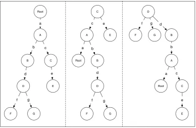
graph of Figure 2.5, illustrates a tree GT with eight vertices and the predecessor
relation:
E ={(root, A),(A, B),(A, C),(B, D),(C, E),(D, F),(D, G)}
A traversal of the tree, in either depth or breadth first order, produces a set of
labels which describe the possibleconnectivity paths starting from the root node. For instance, a depth first traversal of the left-most tree in Figure 2.5 results in:
a →b→d→f a→b →d→g
a→c→e
A transition tree can be created for each node in GT, whereby each node is
set as the root node. The middle and right most trees in Figure 2.5 illustrate the
transition trees for nodes C and D respectively. The depth of a transition tree defines the maximum length of connectivity paths. For instance, if the depth for
Root A C B D F G E a b c d e f g Root A C B D F G E a b c d e f g Root A C B D F G E a b c d e f g
Figure 2.5: Three transition trees, with root nodes set from left to right to Root, C and D.
2.2.3
Graph Compatibility
Two graphs can be compared together in order to establish their compatibility. For instance, graphs encoding 3D objects can be directly compared to establish
object similarity (Maple & Wang, 2004). Graphs G and H are equal only when their respective sets of vertices, labels and edges are equal as follows:
Definition A graph G = (VG, LG, EG) is equal to a graph H = (VH, LH, EH),
written G=H, if an only if VG =VH,LG =LH and EG=EH.
This definition of graph equality is usually relaxed in order to measure the
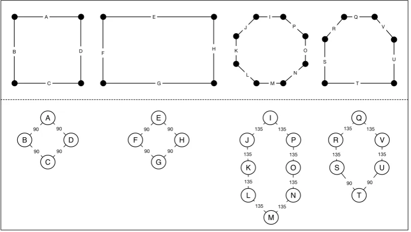
distance between graphs using a variety of metrics. Figure 2.6 illustrates four 2D
shapes with corresponding graphs modelling side connectivity. Nodes represent sides, whereas arcs define a relation specifying which of the sides are connected,
with labels stating the smallest angle subtended between each pair of connected
sides. In this case, a perfectly reasonable distance metric, compares the
cardinal-ity of the elements of the set partition of E when grouped by anglesx∈X. The resulting set partitions are shown in Table 2.1. Using this distance metric, the
first two shapes of Figure 2.6 would appear to be identical, whereas the square
A B C D E F G H I J K L M N O P Q R S T U V A D C B E H G F I P K J 90 90 90 90 L M N O Q V S R U T 90 90 90 90 135 135 135 135 135 135 135 135 135 135 90 90 135 135
Figure 2.6: 2D shapes with their respective graphs, where nodes represent shape sides and edges are labeled with the smallest angle subtended between each pair of adjacent sides.
square {{(A,90, B),(B,90, C),(C,90, D),(D,90, A)}}
rectangle {{(E,90, F),(F,90, G),(G,90, H),(H,90, E)}}
octagon {{(I,135, J),(J,135, K),(K,135, L),(L,135, M),(M,135, N),
(N,135, O),(O,135, P),(P,135, I)}}
house {{(Q,135, R),(R,135, S),(U,135, V),(V,135, Q)},
[image:36.595.116.523.104.334.2]{(S,90, T),(T,90, U)}}
Table 2.1: Set partitions computed according to arc angle values for shapes in Figure 2.6
set partition contains a partition with four arcs at 135 degrees and another with
two arcs at 90 degrees and therefore has elements (in this case angles between
sides) in common with all the three other shapes. The shape distance metric
used here is a heuristic, and therefore not guaranteed to give an optimal
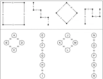
solu-tion on all inputs (in this case 2D shapes) as illustrated in Figure 2.7. Using
this same metric, the first and second shapes are identical, since the respective set partitions both have one partition (90 degrees) of cardinality 4. In order
to further discriminate between these shapes, additional information has to be
stored within the arcs. For instance, direction of rotation as either clockwise or
anti-clockwise can be added and the set partitions originally computed to
distin-guish between relations of various angles can be further refined to now include
A B C D E F G H I J K L M N O P Q R A D C B E F G H I J M L K N O P Q R 90 90 90 90 90 90 90 90 90 90 90 90 90 90 90 90
Figure 2.7: 2D shapes with their respective graphs, where nodes represent shape sides and edges are labelled with the smallest angle subtended between each pair of adjacent sides.
2.3
Point Clouds
A point cloud is a collection of geometric data points within a coordinate
sys-tem. This collection can be viewed as a set, in that order is not important and
no two elements are the same even if these points happen to have exactly the
same properties. In the context of this work, a point cloud is used to describe
a discrete point-based external surface representation. Minimally, it consists of
a collection of geometric points storing per-point position information with no connectivity relation between points. A set embellished only of position
informa-tion is referred to as a raw point cloud. If required, connectivity between points
may be computed by applying some surface reconstruction algorithm to produce
a continuous surface representation. Rapid advancements in acquisition methods
and hardware have resulted in point clouds which can be very large and able to
capture high frequency surface detail, with sizes ranging between 106 and 109
Figure 2.8: A cylinder with an etched band along its centre with (from left to right) increasing number of surface samples. Only the third set of samples provide some information about the etched band.
2.3.1
Point Sampling
At its very basic, a point sample consists of three real numbers defined within
some 3D coordinate space which specify position. A direction vector
represent-ing the surface normal from where the point is sampled is also usually computed.
Figure 2.8 illustrates a cylinder being represented with, from left to right, an
increasing number of points with position and normal information. Additional properties are usually attached to the point depending on how the point is used.
For instance, when used for visualisation purposes, the sample point tries to
cap-ture a very small area on the surface of the object and is therefore augmented with
visualisation properties such as colour, alpha blending and pixel size properties.
Sampling refers to the process of acquiring a discrete set of points
represen-tative of a signal. In this context, the signal can either be a virtual or real scene.
A virtual scene consists of a collection of geometric primitives (e.g. triangles,
spheres), whereas a real scene can be anything physical around us. Whether
vir-tual or real, a sceneSC can be characterised as a set of parametrised 3D surface patches SP and defined as follows:
Definition A smooth parametrised surface patchSP inR3 is a functionx:U ⊂
R2 ⇒R3. As (u,v) varies overU, x(u,v)s traces out a surface patch in R3.
The function x, may represent any function that defines a surface. Figure 2.9 visually illustrates the definition of a surface patch above. For very simple
sur-faces, for instance a plane (continuous and without boundaries), three samples
U
V (u,v)
x x(u,v)
Y
Z
X
Figure 2.9: The functionx traces a surface patch inR3.
for more complex free-form surfaces, many more samples are required to establish
x. In the case of a generic scene, there may exist many sets of surface patches which can describe the scene, all of which might be valid. Given a particular set,
any complex surface patch contained within may be further split into simpler surface patches. Establishing an optimal set of surface patches is in itself a very
active research topic (Cohen-Steiner et al., 2004) and is not discussed here. When sampling, aliasing may occur depending on the sampling frequency
used, where in order to correctly reconstruct an input signal, this needs to be
sampled at least two times the original signal frequency (Oppenheimet al., 1989). The higher the number of samples acquired from a scene, the closer the discrete
point cloud representation is to the surface patch and in the general case the easier
it is to reconstruct (e.g. for visualisation purposes). In the case of Figure 2.8, a
geometric definition of a cylinder with an etched band around it is increasingly sampled from left to right. The additional samples on the right can be used
to improve the reconstruction of the original signal. Whereas in all three cases
there are enough points to parametrically fit the large cylinder and thus the same
cylinder can be reconstructed, given no knowledge of the scene, the more samples
acquired from a surface the higher the confidence that the object in the scene
is a cylinder. Moreover, surface detail such as the band around the cylinder, is
only captured in the third set of samples. In the second set of samples only one
sample is acquired from the band and this can easily be disregarded as noise.
R1
Rn
Viewpoint
S1
Sn
⠇ ⠇
Geometry Primitives
Figure 2.10: Sampling can be done using a ray casting process.
which casts rays towards the objects in the scene. Samples are taken by
intersect-ing rays with visible object surfaces in the scene. In this example the diamond
shape is not sampled since it is occluded by the oval shape. The set of samples
produced from one observer viewpoint is referred to as ascan and is defined using set comprehension as follows:
{r:Ray, sp:SP|Intersect(r, sp)•(Sample(F irstIntersect(r, sp)))}
This set comprehension describes the samples produced by one scan of a
scene. The properties of a point are inserted in the set only if an intersection
exists between one of the rays and the objects (represented as a set of surface
patches, SP) in the scene. The set comprehension returns a set with the position
of first ray surface intersections and depending on the scanner used, possibly other
properties (e.g. colour and normal). The distribution of points depends on the set of raysr. By changing scanner viewpoint (position and/or direction) a new set of rays results in different intersection points within the scene producing additional
samples. In general, in order to acquire samples from all surface patches in
a scene, multiple scans are required, followed by a registration process which
combines these scans into a single coherent point cloud. Given a set I of scans
S whose points have been registered within the same coordinate space, a point cloud is defined as their union S
2.3.2
Acquisition Methods
Many 3D acquisition methods generate point clouds as output. Alternatively,
they may generate range images, analogous to a regular image, which store depth
values along each of regularly spaced rays in space. Range images can easily
be transformed to a point cloud, whereas the inverse is not always possible,
especially in the case when the point cloud corresponds to more than one scan.
Point clouds are used throughout this work, rather than range images, since
these are appropriate for all types of scanners and can be used in all stages of
the 3D acquisition pipeline. Bernardini & Rushmeier (2002) provide an in depth discussion of the 3D acquisition pipeline. All the algorithms presented in this
work take point clouds as their input, hence this section briefly discusses the
different classes of 3D scanners which produce them and a number of properties
associated with them.
Point clouds acquired using a variety of 3D scanners have been used as case
studies in this work. These scanners can be grouped into two main categories,
namely triangulation-based scanners and time-of-flight scanners (Kolb et al., 2009). In order to determine the 3D position of a point, triangulation-based
scanners must observe a specific surface point from at least two separate view-points. Given this constraint is satisfied, the position is determined by computing
corresponding pixels from the two (or more) calibrated viewpoints. This
corre-spondence defines a pair of rays in space, with the intersection of these two
rays determining the 3D position on the surface of the object as illustrated in
Figure 2.11. Triangulation-based scanners are further subdivided by how the
viewpoint is represented. In passive stereo systems (Gross & Pfister, 2011), the
viewpoints contain cameras and no controlled light is introduced in the scene. In
this case, determining correspondence between pixels on the two image planes
equates to searching for pixels with similar features. In many cases this proves to be a difficult task, hence the introduction of active stereo systems which
aug-ment the setup with a spatially temporarily varying projected pattern designed
to introduce features into the scene that make the correspondence problem easier
to solve. Many variants have been developed using this setup including
single-light-stripe systems (Petrov et al., 1998) and structured-light systems (Ribo & Brandner, 2005). For indoor scene acquisition, different scanners have been used
in this thesis, namely Asus Xtion (Asus, 2015), Microsoft Kinect v1 (Zhang,
Viewpoint 2
S1
Sn
Geometry Primitives Viewpoint 1
baseline
Rn_vp1 Rn_vp2
R1_vp1
R1_vp2
image planes
Figure 2.11: Triangulation scanners determine surface samples on a scene by computing corresponding pixels from two viewpoints, which in turn define a pair of rays in space. The intersection point between these two rays results in the surface sample position.
light active stereo. In all cases one of the viewpoints is equipped with a projector
which projects a unique infrared pattern of dots, usually a grid, which an infrared
camera (the second viewpoint) then uses to determine distance from objects.
Figure 2.12 illustrates the point cloud resulting from scanning a keyboard
using the aforementioned scanners. In all three cases the keyboard is represented
by around 20K samples. The top row shows the points sampled but doesn’t
clearly show the quality of the point cloud. In order to illustrate the difference
between the point clouds, the second row shows a triangular mesh computed
over these points. The samples acquired by the Microsoft Kinect (V1) sensor are clearly inferior to the other two sensors. The second and third point clouds
are very similar, with the point cloud acquired via the Structure Sensor being
slightly more accurate, for instance when sampling the large zero key on the
keypad. Figure 2.13 illustrates the point cloud representing the same keyboard
using less samples, resulting from an increase in the distance between the sensor
and the keyboard. The surface details, in this case all the keys, which were visible
before are now lost due to aliasing. Even though sample positions are computed
correctly, not enough samples are available to reconstruct the high frequency
surface details of the original signal. The number of samples representing the keyboard goes down from 20K to 1K when the distance between the scanner and
keyboard is increased five-fold.
Figure 2.12: Point clouds acquired using the Microsoft Kinect, Asus Xtion and Struc-ture Sensor triangulation-based scanners respectively. The Skanect software (Tisserand & Burrus, 2015) is used to extract depth information and carry out tessellation. Mesh-Lab (Cignoniet al., 2008) is used to render both top row point clouds and bottom row triangular meshes.
principles are predominantly used to acquire very large scenes, although some
can also be used for indoor scenes. As opposed to triangulation based scanners
only one viewpoint is necessary to determine ray-object intersections. Funda-mentally, TOF scanners measure the time it takes for a laser, either pulsed or
modulated, to travel to the nearest object in a scene and back along the same
path to a detector built into the scanner. The accuracy of TOF scanners depends
on how accurately the round-trip time can be measured. Recent advances, for
instance scanners using phase-shifting technology, have increased measurement
accuracy (Zhang & Yau, 2006). A popular application of the LiDaR principle
is that of making high-resolution terrestrial maps. Scanners are mounted on
airborne systems in order to generate precise, 3D information of the Earth
sur-face. Each point in the cloud has 3D spatial coordinates representing latitude,
longitude and altitude. Figure 2.14 illustrates different scans produced by TOF scanners. The top row left-hand side point cloud illustrates a 360◦ scan of a green
area at the University of Warwick. The right-hand side point cloud illustrates
part of a scan representing a pre-historic temple in Malta. The bottom row
il-lustrates a 20M samples point cloud of an urban area in Malta acquired via an
airborne LiDaR scanner.
2.3.3
Quality
The quality of a point cloudP can be measured in a number of different ways. For instance, Paulyet al. (2004) present a framework for analysing shape uncertainty and variability in point-sampled scenes using a statistical representation that
quantifies for each point, the likelihood that a surface fitting the data passes through that point. The resulting likelihood and confidence maps are then used
to describe the quality of P. A less elaborate approach to measure the quality of a point cloud is given here, which takes in consideration object clutter and
sample noise. Given a scene SC, decomposed into a set of surface patches SP, the quality of the point cloud representing it is a combination of:
1. the number of observed and acquired patchess ∈SP
2. for eachs ∈SP, the signal to noise ratio in s