Do experts incorporate statistical model forecasts and
should they?
Rianne Legerstee1
Philip Hans Franses Richard Paap
Econometric Institute - Erasmus University Rotterdam
Econometric Institute Report 2011-32 September 30, 2011
Abstract
Experts can rely on statistical model forecasts when creating their own forecasts. Usually it is not known what experts actually do. In this paper we focus on three questions, which we try to answer given the availability of expert forecasts and model forecasts. First, is the expert forecast related to the model forecast and how? Second, how is this potential relation influenced by other factors? Third, how does this relation influence forecast accuracy?
We propose a new and innovative two-level Hierarchical Bayes model to an-swer these questions. We apply our proposed methodology to a large data set of forecasts and realizations of SKU-level sales data from a pharmaceutical com-pany. We find that expert forecasts can depend on model forecasts in a variety of ways. Average sales levels, sales volatility, and the forecast horizon influence this dependence. We also demonstrate that theoretical implications of expert behavior on forecast accuracy are reflected in the empirical data.
Keywords: model forecasts; expert forecasts; forecast adjustment; Bayesian analysis; endogeneity
1We are very grateful to participants of the 31st Annual International Symposium on Forecasting in
Prague on June 26-29, 2011 and to participants of the annual conference of the Netherlands Econometric Study Group in Rotterdam on June 10, 2011 for their helpful comments. Please address correspondence to: Rianne Legerstee, Econometric Institute, Erasmus University Rotterdam, PO Box 1738, 3000 DR Rotterdam, Netherlands, e-mail: [email protected]
1
Introduction
In many forecasting situations there are two forecasts available. First, a statistical model is used to produce a model forecast, which is based on available (past) data and possibly other variables. Second, an expert creates an expert forecast. Usually it is assumed that an expert first looks at the model-based forecast and then decides to make an adjustment and, if so, decides on the size of the adjustment.
The literature on judgmental adjustments to model forecasts is extensive and grow-ing, in particular due to the fact that more detailed factual data become available. Most literature focuses on the quality improvement or deterioration caused by the adjust-ments. In theory, judgmental adjustments by experts could make expert forecasts more accurate than model-based forecasts. One of the main justifications for judgmental ad-justment is that experts can recognize rare events that might influence the variable under consideration but that are too irregular to be incorporated in statistical models (Goodwin, 2000).
A few of the earlier studies on forecast adjustment using actual case study data are Mathews and Diamantopoulos (1986, 1989, 1990, 1992, 1994), Diamantopoulos and Mathews (1989) and Blattberg and Hoch (1990). In general, these authors conclude that forecast adjustments lead to more accurate forecasts on average. More recent work by Fildes et al. (2009), and research based on macroeconomic data in for exam-ple McNees (1990) and Turner (1990), also indicates that in general expert adjustments improve forecasting accuracy. However, all studies suggest that there is room for fur-ther improvement. For example, Fildes et al. (2009) find that for only three out of the four investigated companies judgmental adjustments increased accuracy on aver-age. Furthermore, the above studies all document a general tendency towards making positive adjustments.
There are also studies which report that expert forecasts are not necessarily better than model forecasts. In an extensive study, in which adjusted forecasts made by dif-ferent managers are analyzed, Franses and Legerstee (2010) document that managers
do not deteriorate forecast accuracy at best, but that often model forecasts outperform the expert-adjusted forecasts. Franses and Legerstee (2011b) show that similar results hold for a range of different forecast horizons. These two studies, and also Sanders (1992) and Fildes and Goodwin (2007), suggest that model-based forecasts may need less adjustment and that experts perhaps put too much weight on their own contribu-tion.
In sum, in theory, expert-adjusted forecasts should outperform model-based fore-casts and in some cases they appear to do so. However, there is also evidence that experts can reduce the forecast quality of model-based forecasts. These conflicting findings trigger the natural question: what is it exactly that the experts do? And, how does this behavior result in improvement or deterioration of forecast accuracy?
Although some recent studies have tried to answer these questions, there is no study that takes all possible expert behavior into account. For example, Fildes et al. (2009) and Trapero et al. (2010) focus on positive versus negative adjustments and on the size of the adjustments when they evaluate what kind of forecast adjustments generate more accurate forecasts. But what if experts do not look at the model forecasts at all? In that case they are not making (positive or negative) adjustments and there is no relationship between model and expert forecasts at all. If this is the case, how should we evaluate forecast accuracy? Boulaksil and Franses (2009) used a questionnaire to find out what experts do with the model forecasts and how they create final forecasts. Interestingly, part of the experts state that they do not look at the model forecast before they create a forecast themselves. The empirical results in Franses and Legerstee (2009) emphasize the possibility that model forecasts are only partially taken into account in creating the expert forecasts.
This leads to the next natural question: what would be optimal for experts to do? How should they optimally incorporate the model forecasts in the final forecasts? A structured discussion of this issue is absent from the current literature on this subject. We believe it is important though, as insight into optimal behavior can guide methods to evaluate and improve forecasts.
In this paper, we therefore focus on the following three questions which we address given the availability of model forecasts, expert forecasts and realizations: (a) Is the final expert forecast related to the model forecast and how? (b) How is this relation influenced by other factors? (c) How does this relation influence forecast accuracy? In this paper we rely on theoretical arguments and we match these with actual data using a model that is new to the literature.
Central to our approach is the relation
EF =α+βM F +I, (1)
whereEF is the final forecast of the expert,M F is the statistical model forecast and
Iis what we will call the intuition of the expert. This equation will turn out to be key to understanding and analyzing expert forecasts. As we will argue, estimating the pa-rameters of this relation provides an answer to the first research question. Interesting cases are when α is close to 0 andβ is close to 1, indicating that the expert closely follows the model forecasts, and whenα and/ orβ deviate from these values consid-erably. Besides the values of these parameters, it is also interesting to examine the relation between intuitionIand the model forecasts. Are there any factors influencing the model forecasts that also influence throughI? If this is the case, one could have evidence for double counting, a phenomenon also described in Bunn and Salo (1996). Relatingαandβ to various factors can provide an answer to our second research question. For these factors one can think of characteristics of the realized data,R, like the average size and volatility ofR, and of personal characteristics of the expert. It is here where we shall introduce our two-level hierarchical Bayes model.
Finally, relating to research question three, we show that the values of α and β, the correlation between I and R, and the correlation between I and M F influence forecast accuracy ofEF. We provide theoretical arguments and we hold that against our empirical data.
As we have actual data for individual forecasters for various variables and various forecast horizons, we propose a two-level Hierarchical Bayes model. Its first level is
an extended version of (1) whereas the second level consists of equations that relate the parameters in (1) to characteristics of the variable being forecasted, of the forecasts and of the experts. Furthermore, we take into account the possible endogeneity of the model forecasts in (1), that is, potential correlation betweenM F andI, which slightly complicates parameter estimation.
For our case study we use a large data set containing model forecasts and expert forecasts of different experts for stock keeping unit (SKU) level sales data of various medical products. We document that values for α and β differ substantially across products and experts. Factors such as average sales level, sales volatility, and forecast horizon appear to influence the size of α and β. We also draw conclusions on the optimal values forαandβin terms of forecast accuracy. As such, our study is the first to relate expert behavior with expert performance using non-experimental data.
The remainder of the paper is structured as follows. In the next two sections we formulate the hypotheses which are the starting point of our data analysis and which follow from theory and previous research. In Section 4 we describe the models that we develop to test the hypotheses. Section 5 describes the data and the results of our case study. The final section concludes.
2
Modeling expert behavior
What is it that experts do with model forecasts when they create their own forecasts and how is this behavior influenced by other factors? We discuss these two questions, where we assume that there are no records available of this behavior, and hence that we have to use the actual forecasts and realizations to answer the questions.
Although most that we put forward in this section is true for any kind of forecasts from experts, we focus in this section on forecasts for SKU-level sales data as this matches our empirical illustration.
2.1
What do experts do with model forecasts?
To refine notation, we define the relation between expert forecasts and model forecasts as
EFt+h|t =α+βM Ft+h|t+It+h|t, (2)
whereEFt+h|tis the expert forecast created at origintfort+h, wherehis the forecast
horizon,M Ft+h|tis the model forecast created at the same origin, for the same variable
and with the same forecast horizon and where It+h|t is the intuition of the expert at
origint. We assume that for allt, E[It+h|t] = 0, where E is the expectation operator.
In later sections we describe and estimate a model for which (2) is our main building block, where we assume availability ofEFt+h|tandM Ft+h|tfort= 1,2, ..., T.
One typical situation captured by this model is when α = 0 and β = 1. This can be seen as the benchmark situation, in which the expert closely follows the model forecasts. On average over time, if the model forecasts increase (decrease) the expert forecasts increase (decrease) by the same amount. The expert forecasts are on aver-age not higher nor lower than the model forecasts (they are unbiased like the model forecasts) and the only differences between model forecasts and expert forecasts are captured by the intuition of the expert It+h|t. It+h|t covers factors that influence the
expert forecasts otherwise than model forecasts. In this situation a forecaster closely follows the model forecasts and apparently trusts the model forecasts, but might decide to increase or decrease the model forecasts based on factors captured inIt+h|t.
A second interesting variant of (2) is whenα6= 0andβ = 1. Although the expert still follows the model closely, the expert forecasts are on average higher (α > 0) or lower (α < 0) than the model forecasts. Thus there is a constant deviation from the model forecasts. The general level of expert forecasts is thus different than that of the model forecasts. A potential reason for constant deviation might be that the expert has another loss function than used by the model (which is typically mean squared error loss). For example, the expert might believe that underpredicting is worse than overpredicting.
Ifα= 0, but0< β <1, the relation between model forecasts and expert forecasts is less strong than when β = 1. A change in the next model forecast dampens the expert forecast in the same direction (on average). The expert feels that the model forecasts move in the right direction but not to the right extent and this results in 0 < β <1. At the same time, asα = 0and E[It+h|t] = 0and assuming the variable
to be forecasted is always positive2, the expert forecasts are on average lower than the model forecasts.
If α = 0 and β > 1, the expert reacts excessively to the model forecasts. On average, the expert forecasts move in the same direction as the model forecasts, but the expert has reasons to believe that the model generally underestimates the trend in the data. Asα= 0, and E[It+h|t] = 0, and the variable to be forecasted is always positive,
the expert forecasts are on average higher than the model forecasts.
Finally, an extreme variant of (2) appears whenβ = 0. Here, the expert does not consider the model forecast at all and the expert forecasts are determined by other fac-tors. In this situation, expert forecasts do not entail judgmental adjustments to model-based forecasts, as the expert gives his or her own independently created forecasts. The expert forecast is equal to the intercept plus intuition.
Of course, there are other variants, like when α > 0 and 0 < β < 1. Here the expert forecasts do not necessarily deviate from the model forecasts (they might on average approximately be the same). The expert only partially follows the model forecasts, and uses corrections via the intercept.
In sum, expression (2) encompasses many of the possible expert forecasting prac-tices and it is a good starting point for our analysis. It would now be interesting if there is any empirical evidence of the values ofαandβ. Recently, more data sets have be-come available containing statistical model forecasts and expert forecasts. Boulaksil and Franses (2009) showed with a questionnaire that 50% of the responding man-agers do not rely on the model forecasts when they create their final forecasts. This
suggests that β is smaller than 1, or, stated differently, closer to 0. In Franses and Legerstee (2009) the parameters in model (2) are estimated using SKU-sales data and it is reported thatβ is close to0.4, on average, and there is a large variety of potential estimated values.
Fildes et al. (2009) and Mathews and Diamantopoulos (1986) show that often the differences between expert forecasts and model forecasts are positive. Fildes et al. (2009) find for their one-step-ahead forecasts of SKU-sales more positive than negative adjustments and they also find that the upward adjustments tend to lead to final expert forecasts that overpredict. Franses and Legerstee (2011a) show that for forecasts with horizons ranging from one to twelve months there are more positive adjustments than negative adjustments. This might capture the preference of a manager to overpredict in order to prevent being out of stock and thus that managers may have a loss function different than that of the model forecasts. If we relate these findings to (2), we could state that for many expertsαis larger than 0, thatβis different from 1, or both.
Ifβ < 1, as is frequently observed, then the observed upward adjustments imply thatαis often larger than 0. Even if there would not be an upward bias in the expert forecasts, a positiveαmakes sense in case of aβsmaller than 1, in order to prevent a downward bias in the final forecasts, assuming that the model forecasts are unbiased. To summarize, we put forward the following two hypotheses
Hypothesis 1 a. Oftenβ 6= 1in (2). b. Whenβ 6= 1, oftenβ <1in (2). Hypothesis 2 a. Oftenα6= 0in (2). b. Whenα6= 0, oftenα >0in (2).
2.2
What causes
β
6
= 1
and
α
6
= 0?
Now that we have an idea about what it is that experts could do with model forecasts and what they might often do, we can look for factors that determine this behavior.
From the questionnaire results reported in Boulaksil and Franses (2009) we learn that managers are quite confident about their own ability to forecast and that they lack confidence in the model forecasts. As products with large sales volumes might be more important to a manager and as predictions for near-by sales are probably more important because of their urgency, the manager might put even less trust in the model in these situations. Boulaksil and Franses (2009) also find that recent volatile sales figures decreases the trust by managers in the model and they feel the need to make even more adjustments, which thus would result in an even lower value forβ. Fildes et al. (2009) investigate if judgmental forecasts improve the forecast accuracy when sales volume volatility is high, but they find evidence of the opposite. These authors suggest that volatile series are more difficult to forecast, but with Boulaksil and Franses (2009) we would argue that it can also be due to excessive adjustment. We therefore hypothesize the following
Hypothesis 3The probability thatβ in (2) deviates away from 1 towards 0 in-creases when
a. the mean of a target variable is higher; b. a target variable fluctuates more;
c. the forecast horizon decreases.
When a manager wants to prevent being out of stock, then higher average sales volumes and more volatility increases the size of forecast adjustments. Furthermore, Franses and Legerstee (2011a) show that adjustments are more often upwards than downwards for all forecast horizons, but that this is most prominent for shorter hori-zons. Hence, we conjecture that
Hypothesis 4The probability thatαin (2) deviates away from 0 increases when a. the mean of a target variable is higher;
b. a target variable fluctuates more; c. the forecast horizon decreases.
In Section 4 we propose an econometric model with which can put these hypothe-ses to a test.
2.3
Experts’ intuition
When the managers do not trust the model forecasts and make their own forecasts, it is quite likely that there are factors which influence both model forecasts and expert forecasts. Managers have stated in the questionnaire reported in Boulaksil and Franses (2009) that they include recent sales figures as input to their forecast adjustments, even though they know that recent sales figures are also covered by the statistical model forecasts. This is in accordance with the lab findings of Goodwin and Fildes (1999), which is that experts do not only look at special events for their adjustments, but they also consider past data. As these past (sales) data are usually also the input for the models used to create the model forecasts, the result would be a correlation between
M Ft+h|t and It+h|t in (2), or stated differently E(M Ft+h|tIt+h|t) 6= 0. So, our final
hypothesis about expert forecasting behavior is
Hypothesis 5M F is often endogenous in (2), meaning E[M Ft+h|tIt+h|t]6= 0.
Note thatM F being endogenous (and thus not exogenous) has two important im-plications. First of all, it tells us something about what the experts do. It shows that experts use the same information as the model forecasts, possibly in the same way, but more likely in another way. The result could amount to double counting, or at least to an inefficient use of information, especially when the model forecasts are optimal in processing that same information.
The second implication of the endogeneity ofM F in (2) has to do with parameter estimation. It is well known that Ordinary Least Squares (OLS) results in an incon-sistent estimate ofβ ifM F is endogenous, see Heij et al. (2004, p. 396-418). This may result in incorrect conclusions about what it is that experts do with model fore-casts. For example, it may seem that there is a strong relation betweenEF and M F
withβ ≈ 1, while in fact the expert does not look at the model forecasts at all, but simply uses the same factors as input for his or her forecasts as the statistical model used when creating the model forecasts. How to deal with this estimation issue is dis-cussed in Section 4. Before we turn to our econometric model, we first discuss various implications of expert behavior on forecast accuracy.
3
Theoretical implications for accuracy
In this section we demonstrate the theoretical link between the behavior of the experts and their forecasting accuracy. To our knowledge this has never been done before in the literature.
To study the implications of deviating from the benchmark α = 0 and β = 1, we need to propose a loss function to evaluate forecast accuracy. We propose to con-sider a variant of the well-known and often used root mean squared prediction error (RM SP E), and this variant is the expected squared prediction error (ESP E) defined by
ESP E=E[(Rt+h−EFt+h|t)2], (3)
whereEFt+h|tis as defined before and whereRt+his the realization att+h. This loss
function is chosen for convenience, and also because it gives implementable optimality results for α, β and I, as the managers only have expected values of sales instead of realized values when they create their forecasts. The conclusions obtained in this section with this loss function can be generalized to other loss functions, such as the mean squared prediction error (M SP E), theRM SP Eand the difference between the
(R)M SP E of the model and that of the expert (D(R)M SP E). If (2) is substituted in (3) we obtain
ESP E=E[(Rt+h−α−βM Ft+h|t)2] +E[It2+h|t]
−2E[((Rt+h−βM Ft+h|t)It+h|t], (4)
where we have used that E[It+h|t] = 0. The expert can influence three factors of the
ESP E, and these areα, β and It+h|t. For each of these we will discuss the optimal
values ofα, β andIt+h|tthat minimizeESP E, and how deviations from the optimal
values will influence thisESP E.
3.1
Optimal settings
For ease of derivation, at first we assume thatM F is exogenous in (2) and thus that E[M Ft+h|tIt+h|t] = 0. Later on we will relax this assumption.
∂ESP E
∂α = 0 gives the value for α that minimizes ESP E, and that is the OLS
estimate of the constant term in equation (2) given by
αopt =E[Rt+h]−βE[M Ft+h|t]. (5)
∂ESP E
∂β = 0and then substituting it with the optimal value forαin (5) gives the optimal
value forβ, that is,
βopt = E[M Ft+h|tRt+h]−E[M Ft+h|t]E[Rt+h] E[M F2 t+h|t]−E[M Ft+h|t]2 = Cov[M Ft+h|t, Rt+h] V[M Ft+h|t] , (6)
where Cov means covariance and V denotes variance. Under the condition that the model forecasts are unbiased relative to expected realizations, thus E[M Ft+h|t] =
E[Rt+h|t], we see that the more E[M Ft+h|tRt+h] differs from E[M Ft2+h|t], the more
βopt differs from 1. However, under the additional condition that E[M Ft+h|tRt+h] =
E[M F2
t+h|t], we obtain that βopt = 1 and αopt = 0. We could call this
addi-tional condition the relative unbiasedness of the model forecasts. What this rela-tive unbiasedness means is perhaps most easily understood by looking at the estima-tors of E[M Ft+h|tRt+h]and E[M Ft2+h|t], which are
P
M Ft+h|tRt+h and
P
M F2
where the summations P
run over a sample of data. The condition is not met if
P
M Ft+h|tRt+h −PM Ft2+h|t < 0, which occurs whenM F is larger thanR
espe-cially for the largerM F, or ifP
M Ft+h|tRt+h−
P
M Ft2+h|t>0, which occurs when
M F is smaller thanRespecially for the largerM F.
To get more insight into this relative unbiasedness we consider an example. Sup-pose we have only two observations (T = 2), with realizations R2 = 5andR3 = 15 and we have two different sets (marked with superscripts) of one-month-ahead model forecasts, namely {M F1 2|1 = 10, M F 1 3|2 = 10} and {M F 2 2|1 = 11, M F 2 3|2 = 9}. The first set of model forecasts is unbiased and relatively unbiased, as P
Rt+h =
P
M Ft+h|t and PM Ft+h|tRt+h = PM Ft2+h|t. The second set of model
fore-casts is unbiased, but not relatively unbiased, because P
M Ft+h|tRt+h = 190 and
P
M F2
t+h|t = 202. We see now that deviations of M F from R have more weight
for largerM F. IfP
M Ft+h|tRt+h −
P
M Ft2+h|t < 0, a value for β smaller than 1 is optimal and ifP
M Ft+h|tRt+h −PM Ft2+h|t > 0, a value for β larger than 1 is
optimal (see (6)).
Finally, let us look at the influence of It+h|t on ESP E. Remember that we
re-strictedI and M F to be uncorrelated. Although it is impossible to derive for It+h|t
what its optimal value is, we can see from (4) that adding intuition is only beneficial for reducing the expected forecast error if R and I are positively correlated (see the negative sign before the third right-hand-side element). To be more precise, it should hold that
2Cov[Rt+hIt+h|t]>V[It+h|t], (7)
which means that the covariance betweenR andI should be larger than half the vari-ance ofI. However, we restrictedI andM F to be uncorrelated and we might assume a strong correlation between R and M F. The stronger the last two are related, the harder it is for I and R to be correlated, while maintaining the exogeneity of M F
in (2). Note that this conclusion supplements the conclusion of Blattberg and Hoch (1990, pp. 890-891), who state that combinations between model and expert forecasts
will be more accurate than the model or expert forecasts separately if the intuition of the expert is related to the true values.
If we relax the exogeneity assumption that E[M Ft+h|tIt+h|t] = 0, matters get more
complicated. Working in the same way as for the case of exogenous model forecasts, we find the following value ofαthat minimizesESP E:
αopt =E[Rt+h]−βE[M Ft+h|t], (8)
which is the same as before, and the following value ofβ that minimizesESP E:
βopt = E[M Ft+h|tRt+h]−E[M Ft+h|t]E[Rt+h]−E[M Ft+h|tIt+h|t] E[M F2 t+h|t]−E[M Ft+h|t]2 = Cov[M Ft+h|t, Rt+h]−Cov[M Ft+h|tIt+h|t] V[M Ft+h|t] , (9)
which is different than before. If we assume the model forecasts to be unbiased and relatively unbiased we obtain
αopt = Cov[M Ft+h|tIt+h|t] V[M Ft+h|t] E[M Ft+h|t], (10) βopt = 1− Cov[M Ft+h|tIt+h|t] V[M Ft+h|t] . (11)
We can see that the optimal value ofβis now negatively correlated with the covariance betweenM F and I. The higher the correlation, the lower βopt should be, and vice
versa. This is intuitively understandable, as a high covariance between M F and I
and a highβ (equal to 1 or higher) would result in double counting. In that case the expert fully takes the model forecasts into account, but also lets the final forecasts be influenced by the same factors that determine the model forecasts.
At the same time, a higher covariance betweenM F andIshould result in a higher value forαbecause of a lower value forβ. As E[It+h|t] = 0, αshould in this case be
different from 0 to make the expert forecasts unbiased.
The question now is: how beneficial is it for the expert to relate intuition to the model forecasts and to what extent? If we look at (4), our initial idea could be that a high correlation betweenRandI and a low, preferably negative, correlation between
M F and I is best for expert forecast accuracy. Assuming unbiased and relatively unbiased model forecasts this would result in aβopt larger than 1 and a negativeαopt.
However, the gains in forecast accuracy achieved when I is positively related to R
and when it is negatively related toM F are offset by the second term in (4), that is, a higher variance ofIincreases the forecast error. Furthermore, the moreRandM F are related, the harder it is to letIbe positively correlated withRand negatively correlated withM F.
If R and M F are not that strongly related, it might be best to choose It+h|t in
such a way that it corrects for the mistakes that the model forecasts make, thus to let factors that wrongly influenceM F negatively influenceI. This results in a negative correlation between I and M F and a positive correlation between I and R. In that caseβshould be larger than 1.
In short, we have to take a closer look at the last two terms in (4). We observe that adding intuition is only beneficial if
2E[(Rt+h−βM Ft+h|t)It+h|t]>V[It+h|t]. (12)
Hence, a necessary condition is that intuition is positively correlated with (Rt+h −
βM Ft+h|t), which implies that E[Rt+hIt+h|t] > βE[M Ft+h|tIt+h|t]. Thus forβ = 1,
the correlation between intuition and realization has to be larger than the correlation between intuition and model forecast.
3.2
Implications and hypotheses
Before we summarize the above in a set of statements we define the following condi-tions:
E[Rt+h] =E[M Ft+h|t], (13)
E[M Ft+h|tRt+h] =E[M Ft2+h|t]. (14)
Furthermore, we generalize the above results to the difference between theESP Eof the model and that of the expert (DESP E), as usually the interest is in deterioration or
improvement of the expert forecasts over the model forecasts. If we obtain a minimum value ofESP Efor particular values ofα,βandIt+h|t, we also obtain an optimal value
of DESP E, meaning that (for given model forecasts) DESP E is at its maximum value.
StatementsIn order to have maximum improvement in expected forecast ac-curacy ofEF overM F it has to hold in (2) that,
a. α = 0, β = 1, and (7) is met forIt+h|t, assuming that (13) and (14) are met
and that E[M Ft+h|tIt+h|t] = 0;
b. α is as in (10), β as in (11), and (12) is met forIt+h|t, if (13) and (14) are
met, but possibly E[M Ft+h|tIt+h|t]6= 0;
c. αis as in (8),β as in (9), and (12) is met for It+h|t, if (13) and (14) arenot
met and possibly E[M Ft+h|tIt+h|t]6= 0.
Note that (7) and (12) are minimum requirements for intuition to be beneficial and forDESP Eto be optimal.
Any deviation from the optimal values forαandβ and from (12) results in higher prediction errors forEF, where the amount of loss of precision depends on the inter-action betweenα,β andIt+h|t. For example, in caseβ is larger than 1, and the model
forecasts are unbiased, relatively unbiased (conditions (13) and (14) are met) and ex-ogenous in (2), it is optimal thatα is smaller than 0. Furthermore, in that case, the correlation between the intuition of the expert and the realized values should be even larger than whenβ equals 1.
Although the described behavior is theoretically the behavior that generates the most accurate forecasts, it is questionable whether an expert can act according to the statements (a) to (c) in practice. The interactions between the various determinants of forecast accuracy, especially when taking into account the possibility that the con-ditions are not met, are quite complex. Furthermore, for a given set of actual model forecasts it might be assumed that conditions (13) and (14) are met approximately and thatRandM F are strongly related in general. Therefore we put forward the following
simpler hypothesis:
Hypothesis 6The improvement in expected forecast accuracy of EF over that ofM F increases when in (2)
a. αis 0 orαgets closer to 0; b. βis 1 orβgets closer to 1;
c. the correlation betweenM F andI decreases; d. the correlation betweenIandRincreases.
For a given data set, for which we do not have reasons to doubt that the conditions as defined in (13) and (14) are met, it might be interesting to test Hypothesis 6.
4
Empirical models
In this section we will explain in detail how a (non-trivial) econometric model can be constructed to validate the components of Hypothesis 6. We first consider expert behavior and then its link with forecast accuracy.
4.1
Model of expert behavior
In this section we propose a model to estimate what the experts do with the model forecasts and which factors influence this behavior. It is a two-level Hierarchical Bayes model, for which the parameters can be estimated using panel data, consisting of model forecasts and expert forecasts for different products and for different time periods.
To meet the typical data format in practice, and also to reduce notational burden, we now introduce a slightly different notation. LetEFi,tdenote the expert forecast created
in period t for case i, where i covers products and forecast horizons. Furthermore,
M Fi,t is the model forecast created in that same period, for that same product and
with the same forecast horizon. LetTi be the number of observations for product and
N product-horizon combinations and thus time series. See Appendix A for a more detailed explanation of the data format. Using this notation we can then write (2) as
EFi,t −M Fi,t =α∗i +β
∗
iM Fi,t+εi,t, (15)
withεi,t ∼ N(0, σε,i2 ). Note that β
∗
i in this model associates withβ−1in (2) andα
∗
i
withαin (2). This expression constitutes the first level of our model.
To correctly estimate the parameters and to see which factors influenceα∗i andβi∗
over t, we add a second level to the model. As α∗i = 0 andβi∗ = 0 are the special benchmark cases in the behavior of experts and the forecast accuracy related to it, we take these as our starting point.
Letzi be a vector containing explanatory variables such as mean and volatility of
the variable being forecasted, we can expand the model with
α∗i = 0 ifPi = 1 α†i =zi0γα+ξi ifPi = 0, (16) and βi∗ = 0 ifSi = 1 βi† =z0iγβ+ηi ifSi = 0, (17)
withξi ∼ N(0, σξ2)andηi ∼ N(0, ση2). Pi andSi are unobserved variables which can
take values 1 and 0. WithP r[Pi = 1] =κiandP r[Si = 1] =λi, we assume that there
is an unconditional probability of sizeκi thatα∗i = 0and that there is an unconditional
probability of λi that βi∗ = 0. Stated differently, with a probability of κi times λi
the expert forecasts of casei follow the model forecasts closely and match with the benchmark situation as described in Section 2.1. Ifα∗i differs from 0 it equalsα†i which is then conditional normally distributed and which depends linearly on the variables in
zi. Ifβi∗ differs from 0 it equalsβ
†
i which is also conditional normally distributed and
which also depends linearly on the variables inzi, but with other parameters (γβ).
conditional probabilities: Pi = 1 ifqi =zi0ψα+νi >0 0 ifqi =zi0ψα+νi ≤0, (18) and Si = 1 ifwi =zi0ψβ +ωi >0 0 ifwi =zi0ψβ +ωi ≤0, (19)
withνi ∼ N(0,1)andωi ∼ N(0,1). Stated differently, the probabilities thatPi = 1
(α∗i = 0) and thatSi = 1(βi∗ = 0) are defined as a probit model withzi as explanatory
variables. We can also write this as
κi = Z ∞ 0 φ(qi;zi0ψα,1)dqi, (20) and λi = Z ∞ 0 φ(wi;zi0ψβ,1)dwi, (21)
whereφ(·;c1, c2)is the probability density function (pdf) of a normal distribution with meanc1and variancec2. Thus, the variables inzi are related toα†i andβ
†
i, but also to
the probabilities thatαi∗ = 0and thatβi∗ = 0. Although we use for all four relations the samezihere, it is of course also possible to use different sets of explanatory variables.
Equations (16), (17), (20) and (21) constitute the second level of our model.
Sofar we have assumed that the error terms in our basic equation (15) are unre-lated to the model forecasts, and thus that the model forecasts are exogenous. It is however very well possible that there is correlation between these two components, as explained in Section 2.3. If this problem is ignored we might find values forβi∗ that are inconsistent. To account for possible endogeneity in the first equation we therefore add the following component to the model, that is,
M Fi,t =µi+δiVi,t+ζi,t, (22)
withVi,tan instrumental variable. Now we have(εi,t, ζi,t)0 ∼M N(0,Ωi), whereεi,tis
both variables and with covariance matrixΩi (which is a2×2matrix). If there is no
correlation betweenεi,t andζi,t, or, stated differently,Ωi(1,2) = Ωi(2,1) = 0, there is
no endogeneity.
Taking everything together, the full final model now reads as
EFi,t −M Fi,t =α∗i +β
∗
iM Fi,t+εi,t, (23)
M Fi,t =µi+δiVi,t+ζi,t, (24)
α∗i = 0 ifPi = 1 α†i =zi0γα+ξi ifPi = 0 (25) βi∗ = 0 ifSi = 1 βi† =z0iγβ+ηi ifSi = 0, (26) Pi = 1 ifqi =zi0ψα+νi >0 0 ifqi =zi0ψα+νi ≤0, (27) Si = 1 ifwi =zi0ψβ +ωi >0 0 ifwi =zi0ψβ +ωi ≤0. (28)
The first two equations are the first level of the model in which the difference between
EF andM F is linked toM F and where possible endogeneity ofM F is incorporated. The second level of the model is given by the other four equations, where the param-eters of the first level are linked to potentially explanatory variables. The benchmark caseα∗i = 0andβi∗ = 0has a key position in this model.
To estimate the posterior results of the parameters of this model, namely
θ = ({βi†}N i=1,{α † i}Ni=1,{µi}iN=1,{δi}Ni=1, γ 0 α, γ 0 β, ψ 0 α, ψ 0 β,{Ωi}Ni=1, σξ2, ση2), the Markov
Chain Monte Carlo (MCMC) methodology, and in particular Gibbs sampling, is used. Technical details on this sampler are presented in Appendix B. We are especially in-terested in the values of parameters{βi†}N
i=1,{α
†
i}Ni=1, γα, γβ, ψα, ψβ and{Ωi}Ni=1, as these represent the behavior of the experts and how this behavior is governed by other factors.
4.2
Evaluating forecasts
The estimated parameters of the model in the previous section can be used to test Hypotheses 1 to 5 about the behavior of experts. However, we are also interested in what the experts should do, which is the subject of the Statements and Hypothesis 6. As the Statements follow straightforwardly from optimization of the forecast accuracy target function there is no need to test it. However, the rules to follow according to these statements are quite complex and therefore Hypothesis 6 comprises a simpler set of rules to follow. To test the validity of Hypothesis 6 we need one additional model which we propose in this subsection. In this model we use a measure of the forecast precision of the expert as compared to the forecast precision of the model and relate this with variables as mentioned in Hypothesis 6.
LetDRM SP Eibe the improvement in root mean squared prediction error ofEFi,t
overM Fi,t, thus
DRM SP Ei = r 1 Ti X (Ri,t−M Fi,t)2− r 1 Ti X (Ri,t−EFi,t)2. (29)
We use this criterium instead of DSP E to reduce variability. With the regression model
DRM SP Ei =ri0ϑ+ιi, (30)
it is possible to test which factors influence forecast improvement.
First of all, we want to test if α∗ = 0 indeed increases forecast improvement, as compared to cases whereα∗ 6= 0. This is the first part of Hypothesis 6a. We also want to test if, assuming thatα∗is different from 0, a smaller value ofα∗in absolute sense is beneficial to the forecast improvement (second part of Hypothesis 6a). Therefore, we consider the estimates ofPi and the estimates of|α
†
i(1−Pi)|as explanatory variables
in (30), where we use the posterior means forPi andα†. We call the first variable in
the remainder of this paper ‘No intercept’ and following Hypothesis 6a we expect this variable to have a positive effect. The second variable is called ‘Size intercept’ and following Hypothesis 6b we expect this variable to have a negative effect.
To test ifβ∗ = 0(orβ in (2) equals 1) increases forecast improvement compared toβ∗ 6= 0(first part of Hypothesis 6b), we add the posterior mean forSi. The second
part of Hypothesis 6b, namely that a larger absolute value of β∗ decreases forecast improvement, is tested by using the estimates of|βi†(1−Si)|as an explanatory variable,
where we again use the posterior mean forSi and we use the posterior mean forβ
†
i.
These variables will carry the labels ‘Relation MF’ and ‘Size relation MF’ and we expect the first variable to have a positive effect and the second variable to have a negative effect.
Hypothesis 6c states thatDRM SP Eincreases if the correlation betweenM F and
I decreases. To test this we useρΩ,i = Ωi(1,2)/
p
Ωi(1,1)Ωi(2,2)as an explanatory
variable, where we use the posterior mean for Ωi, label ρΩ,i ‘Endogeneity’, and we
expect a parameter with a negative value.
Finally, by including in (30)ρεR,i = corr(εi,t, Ri,t)Hypothesis 6d is considered.
That is, the correlation between the estimated errors of (15) and the realized values of the variable of interest is used to see if correlation between the expert intuition and the true values increases the forecasts. The errors of (15),εi,t, are estimated as
EFi,t−M Fi,t−α
†
i(1−Pi)−β
†
i(1−Si)M Fi,t, using the posterior means forα
†
i,β
†
i,
Pi andSi. The variableρεR,i is labeled ‘Intuition’ in the remainder of the paper and
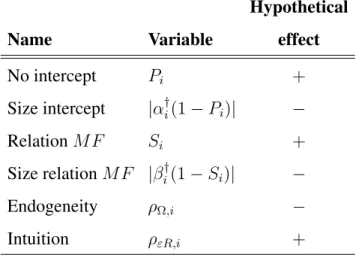
following Hypothesis 6d we expect it to have a positive effect in (30). Concluding, we have for (30) the set of six explanatory variables
r0i = [1, Pi, |α
†
i(1−Pi)|, Si, |β
†
i(1−Si)|, ρΩ,i, ρεR,i]. (31)
See Table 1 for an overview of the variables inri, the names of the variables and for
the hypothetical sign of the parameters in (30) following Hypothesis 6.
5
Empirical results
To illustrate the usefulness of our two models we make use of an extensive panel data set. The data set covers SKU-level sales data and is described in detail in the next subsection. In Subsections 5.2 and 5.3 the results of our analysis are discussed.
5.1
Data set
For our case study we use monthly sales data of a large pharmaceutical company. The company has its headquarters in The Netherlands, and has local offices in various countries. The company uses an automated statistical package to create forecasts using lagged sales figures as the only input. Each month model selection and parameter estimation are updated, whereby the package uses techniques such as Box-Jenkins and Holt-Winters. These model forecasts are then sent to the managers in the local offices, after which they quote their own forecasts.
We have at our disposal model forecasts, manager forecasts and actual sales figures for November 2004 through November 2006, with for 1-step-ahead forecasts a maxi-mum of 25 triplets per product (medicine), for 2-step-ahead forecasts a maximaxi-mum of 24 triplets and so on. We have a total of 7250 time series for 1167 different products in 7 different categories, sold in 36 countries. For each series, two observations are lost, because of the instrumental variable we used (see below). Therefore, for each series we have a minimum of 10 observations, a maximum of 23 observations and the forecast horizon ranges from 1 to 7 months.
In the notation of Appendix A and Table A.1 this means that we haveN = 7250,
J = 1167and the maximum ofHj forj = 1, ..,1167is 7. Because there is one
man-ager per country responsible for the expert forecasts, we haveM = 36. Furthermore,
t= 1corresponds with the month October 2004 andT corresponds with October 2006 (forecast origin).
As an instrumental variable in (22) we need a variable that correlates with the model forecasts, but not with the expert forecasts, see, for example, Heij et al. (2004,
p. 396-418). The instrumental variableVi,t that we use isRi,t−(h+1) −M Fi,t−(h+1), whereRi,t−(h+1) concerns case i in montht −(h+ 1) and M Fi,t−(h+1) is the asso-ciated model forecast.3 So, as instrumental variable we use the most recent forecast
error of the model forecast that has the same forecast horizon and that is known at the moment of forecast creation. Franses and Legerstee (2009) show that this variable often does not correlate much with the difference between model forecasts and expert forecasts. Because we do think it correlates with model forecasts (because of the way model forecasts are created), we believe that expert forecasts and this instrument are not strongly correlated.
The variables that we use as explanatory variables in (16), (17), (20) and (21) and included in vectorzi are average sales volume, sales volatility and dummy variables
for the forecast horizon. We also include dummy variables for the country (and by that for the manager responsible for forecasting) and dummy variables for the category of a product.
The optimal values forα andβ depend on conditions (13) and (14) as defined in Section 3, which are conditions on the bias and relative bias of the model forecasts. Furthermore, the more the conditions are not met, the less likely it is that Hypothesis 6 is true. Therefore, it is first useful to find out to what extent these conditions are met for our data. To get insight into this we tested for each caseiif there is a significant difference between the mean ofM F and the mean ofR (condition (13)) and if there is a significant difference between the mean ofM F timesR and the mean ofM F2
(condition (14)). For this, we used the common small-sample test for comparing two population means as described in Wackerly et al. (2002). We find that condition (13) is rejected in about 17% of the cases and condition (14) in 6% of the cases, where we use a 5% significance level. The test requires the samples to be drawn from a normal distribution. According to the Jarque-Bera test, the hypotheses of normality 3We use the same notation as in Appendix A. Thus forM Fthe second subscript indicates in which
period the forecasts are created. In case ofRthe second subscript indicates in which period the forecasts are created to which the realization belongs, thus it is the realization of periodt−1.
are not rejected in only 61% of the cases. In again around17% of these cases (for which both null hypotheses of normality are not rejected) condition (13) is rejected at the5% significance level. To test the second condition, both theM F timesRsample and the M F2 sample need to be drawn from a normal distribution. Here, according to the Jarque-Bera test, the hypotheses of normality are not rejected in 53% of the cases and in around7% of these cases (for which both null hypotheses of normality are not rejected) condition (14) is rejected at the5%significance level. Thus although the normality assumption does not always hold, we can state with fair confidence that condition (13) holds in about83%of the cases and condition (14) holds in about93% of the cases.
5.2
Expert Behavior
To estimate the parameters of the model described in Section 4.1 we generate 80,000 iterations of the Gibbs sampler as described in Appendix B. The first 40,000 iterations are used as burn-in sample, and of the last 40,000 iterations every 10th draw is retained and used to calculate mean and standard deviation of the draws. Iteration plots are inspected to check for convergence and are available upon request.
[INSERT FIGURE 1 ABOUT HERE]
The probability that β∗ = β − 1 = 0 is varying, which can be seen from the histogram in Figure 1 showing the posterior means forSi fori= 1, ..., N. The largest
group of cases (2254) has a probability of less than 0.1 that βi∗ = 0. All the other cases have probabilities that are equally spread between 0.1 and 1. 2718 cases have a probability higher than 0.5, indicating that in less than 40% of the casesβ in (2) is likely to be close to 1.
Figure 2 shows a histogram of the posterior means forβi† for which the posterior mean forSi <0.5and for which the posterior mean for−1 < β
†
i < 1. The smallest
βi† is estimated as -1.14 and the largest is 1.5, but only 11 of the estimated βi† are below -1 and only 17 above 1. In the remainder of this section, we useI[Si < 0.5]β
† i as estimatedβi∗andI[Pi <0.5]α † i as estimatedα ∗
i, whereI[·]is an indicator function
which takes a value 1 if the expression between brackets is true and 0 otherwise and with posterior means for Si, β
†
i, Pi and α
†
i. We find that 2406 of the 4532 β
∗
i
values, that are estimated to be different from 0, are positive. Thus although part a of Hypothesis 1 seems to hold for this data set, part b of this Hypothesis is not supported:
β is often different from 1, but when it is different from 1, it is just as likely smaller than 1 than it is larger than 1. However, we do see a fatter tail to the left than to the right:βis more often much lower than 1 than much higher than 1. Finally, note thatβ
is not often close to 0, indicating that almost all managers producing forecasts in this data set look at the model forecasts to some extent.
[INSERT FIGURE 3 ABOUT HERE]
Figure 3 shows a histogram of posterior means forPi fori= 1, ..., N. We see that
the probability thatα∗ =α = 0is often very high. In only 1030 of the 7250 cases the probability is lower than 0.5 and in 5469 cases it is higher than 0.9. Thus, part a of Hypothesis 2 does not seem to hold: not often isα 6= 0and is there a constant bias in the expert forecasts as compared to the model forecasts.
[INSERT FIGURE 4 ABOUT HERE]
Figure 4 shows a histogram of posterior means for α†i for the cases for which the posterior mean forPi <0.5and for which the posterior mean for−200 < α
†
i <4000.
α†i’s are smaller than -200, but still 135 are larger than 4000. Thus, looking at the histogram and at the values not included in the histogram, we can conclude that the estimatedα†i’s are strongly positively skewed. Only in 44 of the cases is the estimated
αnegative, supporting part b of Hypothesis 2: when αis different from 0, it is often positive.
We observe that the first two hypotheses (1 and 2) are only partly validated. But to what extent are the expert forecasts positively biased, as is often found in previous research (see Section 2.1)? This is the case whenα∗ is larger than 0, whileβ∗ is 0 or also larger than 0, or whenβ∗ is larger than 0, whileα∗ equals 0. We find that in only 2516 cases this seems to hold, which is a little over one third of the cases.
To see if the deviations ofβ∗ from 0 follow the rules that hypothetically optimize the forecast improvement ofEF over M F, we calculate the correlation between the posterior mean forβi∗ andβi,opt =
Cov[M Fi,t,Ri,t]−Cov[M Fi,tIi,t]
V[M Fi,t] fori = 1, ..., N. In
Sec-tion 3 we derived that the optimal value ofβiis given by this fraction in (9). We obtain
a positive correlation of 0.11.
To get more insights, we also counted how often the posterior mean forβ∗ is posi-tive while(Cov[M Fi,t, Ri,t]−Cov[M Fi,tIi,t])> V[M Fi,t]plus how often the posterior
mean forβ∗ is negative while(Cov[M Fi,t, Ri,t]−Cov[M Fi,tIi,t]) < V[M Fi,t]. This
appears to occur in 37% of the cases. The exact opposite is true in only25% of the cases. Thus, according to (9), in25% of the casesβ∗ has the wrong sign, while37% has the correct sign. The remaining 2719 cases have a probability of50% or higher thatβ∗ = 0. For those cases, the difference between βi,opt and 1 is on average0.69,
andβi,opt varies between−51.25and27.94with a standard deviation of1.80. For the
complete data set these values are 0.77 (average difference from 1), −51.25 (mini-mum),33.13(maximum) and1.89(standard deviation). This all gives the impression that there are managers who recognize whenβshould be different from 1 and in which direction it should be different.
We also formulated hypotheses (3 and 4) about factors that might influence the value ofαand β. To find out to what extent these hypotheses are valid for our data,
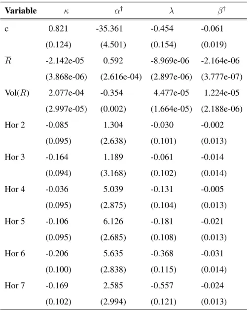
we have to take a look at the posterior means for the parameters in the second level of the model, that is, γα, γβ, ψα, ψβ. Part of the estimated coefficients can be found in
Table 2. First of all, we see support for part a of Hypothesis 4, that is, the average size of sales is positively related withαin (2). We find very strong posterior evidence that both the probability thatα∗ is different from 0 and the level ofα† increase with the average size of sales.
[INSERT TABLE 2 ABOUT HERE]
We see that sales volatility has an opposite effect. The higher the volatility, the lower the probability that α∗ differs from 0 and the lower the value of α†. For both effects there is very strong posterior evidence. This contradicts part b of Hypothesis 4, as we expected that more volatile sales would make a manager to overpredict in order to prevent running out of stock.
Furthermore, we see that forecasts with a horizon of 2 to 7 months have on average a lower probability thatα∗ equals 0 as compared to forecasts with a horizon of just 1 month, with the horizon of 6 months having the lowest estimated coefficient. We also see a parabolic effect of the forecast horizon onα†, with the highestα† for forecasts for 5 and 6 months ahead. Although this seems to contradict part c of Hypothesis 4, for this data these results are perfectly explainable. The management of the firm from which we use the forecasting and sales figures informed us that the 6-month horizon is an important planning horizon. This importance probably results in a suboptimal value forα.
Forβ we find a significantly negative effect of average sales volume on the prob-ability that β∗ is 0 and also a significantly negative relation between average sales volume and β†, both supporting Hypothesis 3a. However, we have to keep in mind that Hypothesis 3 was based on Hypothesis 1b stating thatβ† would be smaller than 0, and that this hypothesis has already been shown to be incorrect: β† is often larger than 0. Thus, as long asβ†is smaller than 0, it moves in the expected direction when
average sales volume increases, but whenβ†is larger than 0, it moves in the same, but now unexpected direction. We calculated the average of(βi†)2 differentiated to each of the variables in zi to see if the variables had an influence on β
†
i moving away or
towards 0, but found only insignificant results. This confirms that the found relations are robust to a change of sign ofβi†.
An increase in the volatility of sales results in a higher probability thatβ∗equals 0 and in an increase inβ†. As with the influence onα, this is not in line with what we hypothesized.
Finally, we see that the longer the forecast horizon the smaller the probability that
β∗ = 0and thatβ†is smallest for a forecast horizon of 6 months. This is in line with part c of Hypothesis 3, again modified for this data set, because the 6-month horizon is an important planning horizon.
The dummy variables for countries (and thus managers) and for medicine cate-gories included in zi are often significantly related to the four dependent variables4.
Thus, on the basis of these results specific managers can be addressed when their α
and/orβvalues are not optimal for (part of) their forecasts and can be given feedback. We are also interested in the correlation betweenM F andI in (2). Hypothesis 5 stated that expert forecasts are often related to external factors which are also related to the model forecasts (endogeneity ofM F in (2)). With Hypothesis 6 we stated that a lower or more negative correlation betweenM F and I in (2) might be beneficial to forecast accuracy. In order to evaluate the correlation between M F and I of the expert forecasts we first have to address two issues. First, we need to know if the instrument, which is the most recent model forecast error known at the moment of forecast creation, is a relevant instrument. We find that in more than 70% of the cases the posterior mean forδin (22) is significantly different from 0, so we can conclude that we used a fairly relevant instrument.
Second, we need to know if the instrument is a valid instrument, that is, is it 4The estimated coefficients for these dummy variables are not shown here, but are available upon
unrelated to expert forecasts? To that extent, we calculate the correlation between the estimated error terms in the first level of the model, εi,t, and the instrument. We
find that the correlation in 2451 cases is<−0.3and in 572 cases is>0.3. Thus, the estimatedβi† might be over- or underestimated and this might give a false impression on what it is the managers do. However, it is hard to find a better instrumental variable for this data set and the validity is certainly not completely rejected.
[INSERT FIGURE 5 ABOUT HERE]
The endogeneity in (2) can now be measured by the correlation in the posterior mean forΩi, that is, by the posterior mean forρΩ,i = Ωi(1,2)/
p
Ωi(1,1)Ωi(2,2)for
alli. The estimated correlations are depicted in Figure 5. The result is surprising. We might expect positive correlations, indicating that factors influencing model forecasts influence the expert forecasts in the same way, resulting in double counting. However, we mainly find negative correlations (in almost 90% of the cases). This would mean that factors influencing the level of model forecasts have an opposite effect on expert forecasts. In Hypothesis 6c we stated that such a negative correlation would benefit the forecast improvement of the expert forecasts over that of the model forecasts. In sum, it seems that the experts are properly adjusting model forecasts, but to what extent this is useful will be discussed in the next section.
[INSERT FIGURE 6 ABOUT HERE]
Finally, it might be interesting to take a look at the correlation between the esti-mated error terms of the first level of the model, εi,t, and realized sales, as we have
seen that this influences the forecast accuracy too. A histogram of these correlations can be found in Figure 6. The correlations are pretty much symmetrically centered around 0, with just a little more positive correlations than negative. This time, it would be preferred that the correlations is positive, see equation (4) and Hypothesis 6.
How-ever, the more model forecasts and realized values are related, the more difficult it is to add intuition to the model forecasts that is negatively related to model forecasts and positively related to the realized values. As we almost always see a negative endo-geneity, this might explain why we also often see a negative relation between realized values and intuition. Probably the managers too often wrongly correct the model fore-casts using factors also influencing these model forefore-casts, resulting in intuitionIbeing negatively correlated with the realized valuesR.
5.3
Forecast Evaluation
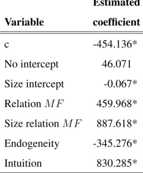
In Table 3 we give the estimated coefficients of model (30). First of all, we see that an expert who produces forecasts withα = 0, β = 1and no correlation between the residuals in (2) and the model forecasts and between the residuals in (2) and realized sales, performs on average better than the model. This can be seen from the sum of the estimated constant c and the estimated coefficients for the variables No intercept and Relation MF being positive. An expert who produces forecasts withα different from 0, β different from 1, but not larger than approximately 1.51 or smaller than approximately 0.49 and the correlations equal to 0, produces on average less accurate forecasts than the model. These values for the variables, that is, No intercept, Relation MF, Endogeneity and Intuition equal to 0, Size intercept positively valued and Size relation MF smaller than 0.51, multiplied by the estimated coefficients and summed up together with the estimated constant c, result in a negativeDRM SP E.
[INSERT TABLE 3 ABOUT HERE]
A decrease in the probability that α = α∗ = 0or in the probability thatβ∗ = 0 (equivalent toβ = 1) both decrease on average the forecast accuracy of the expert fore-casts as compared to the model forefore-casts. This confirms parts a and b of Hypothesis 6. Furthermore, we see a significantly negative coefficient for the size of the parameter
α†which supports the second part of Hypothesis 6a.
The fifth estimated coefficient is not in line with Hypothesis 6b. According to this estimated coefficient,β†moving away from 0 results on average in an increasing DRMSPE. Note however, that the variable ‘Size relation MF’ has to be larger than 0.518 in order to make up for the loss in accuracy due to S 6= 1. DRMSPE is on average approximately 460 higher for S = 1 than for S = 0, ceteris paribus, and only when|βi†(1−Si)| > 0.518is this same level of forecast accuracy improvement
achieved. Of the 7250 cases, this happens only139times (looking at posterior means for the parameters), which is in less than2%of the cases, thus in general it is still more beneficial to haveβ = 1thanβ 6= 1.
The fact that values of β further away from 1 result in more accurate forecasts as compared to model forecasts than values ofβcloser to 1, has probably to do with the correlation between the optimalβand the bias and relative bias in model forecasts and the endogeneity of the model forecasts in (2). This is confirmed by the fact that we found a positive correlation between the optimal value of βi and the estimated βi∗ in
the previous section.
The next two estimated coefficients, corresponding to the correlation of intuition with model forecasts and of intuition with realized values, have the expected signs again. Hypotheses 6c and 6d get support as we find that a lower correlation between
M F and I increases the forecast accuracy of expert forecasts and a higher correla-tion between intuicorrela-tion and realized sales increases the forecast accuracy of the expert forecasts.
Recall though from Section 3 that it is probably hard to achieve both a negative (or lower) correlation between intuition and model forecasts and a positive (or higher) cor-relation between intuition and realized values, as model forecasts and realized values should be strongly related. Therefore we are interested to see how often the intuition of the expert increases the forecast accuracy relative to the model forecasts. According to the model this is the case when the sum of the variables Endogeneity and Intuition both multiplied by its estimated coefficient is positive. We find this to be true in77%
of the cases.
We can also look at (12), where we presented the theoretical condition under which intuition improves forecast accuracy. To test how often this is the case for our data we use2[Cov(Ri,t, εi,t)−βCov(M Fi,t, εi,t)]>Var(εi,t)for alli, with posterior means for
εi,t. We find that only in953cases this inequality holds, and thus only in approximately
13%of the cases is intuition helpful in improving forecast accuracy.
We can conclude, at least for this data set, that the rules to follow for an expert formulated in Hypothesis 6 are a bit too simple and general. There seem to be experts who do recognize the situations in which the model forecasts are (relatively) biased and who are able to correct, at least partly, this bias. But, on average, an expert who does follow the rules formulated in Hypothesis 6 does perform better than the model and there are not many experts able to improve on the performance of this set of rules by choosing alternative values forαandβ. Furthermore, it seems hard to improve the model forecasts by adding intuition.
6
Conclusions
Expert forecasts, created once statistical model forecasts are available, are quite often discussed in the literature, but still not much is known about how expert forecasts are created. Often the expert forecasts are analyzed on their forecasting performance with-out a proper analysis of what it is the experts actually did. In this paper we formulated hypotheses about the behavior of experts and about the impact of that behavior on forecast accuracy. We proposed a model to find out how expert forecasts are created in relation to model forecasts and to find out which factors influence this behavior. We proposed a novel and innovative two-level Hierarchical Bayes model in which we also take into account that the model forecasts might be endogenous. The observed behavior could then be linked to forecasting performance.
We applied this model to a large data set consisting of model and expert forecasts and realizations of SKU-level sales data. The results for our data set were interesting
and sometimes quite surprising. We found that in about one third of our expert fore-casts there is a structural upward bias. There might be a bias in expert forefore-casts as compared to model forecasts, but at first it is unclear whether this is because the expert adds to the model forecasts or because the expert does not look at the model forecasts and creates own independent forecasts. We found that in approximately 37% of the cases there is a one-to-one relation between model forecasts and expert forecasts. In 50% of the remaining cases the expert reacts excessively to the model forecasts and in the other 50% of the remaining cases the expert only partially takes the model forecasts into account, if at all.
The intercept and the coefficient in the linear relation between expert forecasts and model forecasts were significantly influenced by factors such as average sales volume, sales volatility and forecasting horizon.
We furthermore found that the experts often take other factors into account that also influence the model forecasts. However, often this makes the expert forecasts to deviate in the opposite direction than that the model forecasts were influenced. Thus, we often find endogeneity of the model forecasts, or, to be more precise, a negative cor-relation between the model forecasts and the error terms in the linear cor-relation between expert forecasts and model forecasts. Finally, we found different kinds of relations between the intuition of the experts (other factors than model forecasts influencing the expert forecasts) and the realized sales values.
Theoretically, when the model forecasts are unbiased and relative unbiased as com-pared to the realized values (see Section 3), then expert forecasts which are related to model forecasts in a linear relation with coefficient equal to 1 and intercept equal to 0, would be most accurate as long as intuition and model forecasts are unrelated. However, we find in our data set that the conditions for this (unbiasedness and rela-tive unbiasedness of the model forecasts) are not always met, and that some experts are probably able to recognize this and correct for it. Furthermore, as soon as endo-geneity of the model forecasts is introduced (correlation between intuition and model forecasts), things get more complicated and it is harder to draw straightforward
con-clusions about the optimal values of the coefficients and of the correlation between the residuals and model forecasts and of the correlation between the residuals and realized values. In general, experts who follow some simple rules, which optimize forecast performance under optimal circumstances, outperform the model forecasts in our data set. However, some experts who deviate from these rules, especially those for which
β is further away from 1 and for which the error terms are negatively related to the model forecasts, also perform very well. We found that this has probably to do with the fact that these experts have to deal with poor model forecasts.
There are three main challenges in this area of research. The first is to apply the techniques described in this paper to other data sets. Our results are interesting and very informative, but are limited to the sales data of one company. It would be worth-while using (sales) data from other companies or from other research areas, such as macroeconomics, to see if our results extend to other situations too.
The second challenge is to find and use appropriate instruments to deal with the endogeneity of model forecasts. Although we seemed to have done a pretty good job in our data set, the instrument we used is probably not perfect and this might influence the conclusions that we have drawn. In new research the most difficult task, besides finding a useful data set, is probably to find appropriate instruments.
Finally, in many forecasting situations only expert forecasts are available to the re-searcher and no model forecasts. It would be interesting to investigate ways to retrieve these model forecasts from the available data.
References
Blattberg, R. and Hoch, S. (1990). Database models and managerial intuition: 50% model + 50% manager. Management Science, 36(8):887–899.
Boulaksil, Y. and Franses, P. (2009). Experts’ stated behavior. Interfaces, 39(2):168– 171.
Bunn, D. and Salo, A. (1996). Adjustment of forecasts with model consistent expec-tations. International Journal of Forecasting, 12:163–170.
Diamantopoulos, A. and Mathews, B. (1989). Factors affecting the nature and effec-tiveness of subjective revision in sales forecasting: An empirical study. Managerial and Decision Economics, 10:51–59.
Fildes, R. and Goodwin, P. (2007). Good and bad judgement in forecasting: Lessons from four companies. Foresight: The International Journal of Applied Forecasting, 8:5–10.
Fildes, R., Goodwin, P., Lawrence, M., and Nikolopoulos, K. (2009). Effective fore-casting and judgmental adjustments: An empirical evaluation and strategies for im-provement in supply-chain planning.International Journal of Forecasting, 25:3–23.
Franses, P. and Legerstee, R. (2009). Properties of expert adjustments on model-based SKU-level forecasts. International Journal of Forecasting, 25:35–47.
Franses, P. and Legerstee, R. (2010). Do experts’ adjustments on model-based SKU-level forecasts improve forecast quality? Journal of Forecasting, 29(3):331–340.
Franses, P. and Legerstee, R. (2011a). Combining SKU-level sales forecasts from models and experts. Expert Systems with Applications, 38:2365–2370.
Franses, P. and Legerstee, R. (2011b). Experts’ adjustment to model-based SKU-level forecasts: Does the forecast horizon matter? Journal of the Operational Research Society, 62(3):537–543.
Goodwin, P. (2000). Improving the voluntary integration of statistical forecasts and judgement. International Journal of Forecasting, 16:85–99.
Goodwin, P. and Fildes, R. (1999). Judgmental forecasts of time series affected by special events: Does providing a statistical forecast improve accuracy? Journal of Behavioral Decision Making, 12(1):37–53.
Heij, C., de Boer, P., Franses, P., Kloek, T., and van Dijk, H. (2004). Econometric Methods with Applications in Business and Economics, chapter 5.7, pages 396–418. Oxford University Press.
Mathews, B. and Diamantopoulos, A. (1986). Managerial intervention in forecast-ing: An empirical investigation of forecast manipulation. International Journal of Research in Marketing, 3:3–10.
Mathews, B. and Diamantopoulos, A. (1989). Judgemental revision of sales forecasts: A longitudinal extension. Journal of Forecasting, 8:129–140.
Mathews, B. and Diamantopoulos, A. (1990). Judgmental revision of sales forecasts: Effectiveness of forecast selection. Journal of Forecasting, 9:407–415.
Mathews, B. and Diamantopoulos, A. (1992). Judgmental revision of sales forecasts: The relative performance of judgementally revised versus non revised forecasts.
Journal of Forecasting, 11:569–576.
Mathews, B. and Diamantopoulos, A. (1994). Towards a taxonomy of forecast error measures- a factor-comparative investigation of forecast error dimensions. Journal of Forecasting, 13:409–416.
McNees, S. (1990). The role of judgment in macroeconomic forecasting accuracy.
International Journal of Forecasting, 6:287–299.
Sanders, N. (1992). Accuracy of judgemental forecasts: A comparison. Omega, 20:353–364.