Thermodynamics of ice interfaces and structures within a coarse grained model of water

warwick.ac.uk/lib-publications

A Thesis Submitted for the Degree of PhD at the University of Warwick

Permanent WRAP URL:

http://wrap.warwick.ac.uk/90109

Copyright and reuse:

This thesis is made available online and is protected by original copyright.

Please scroll down to view the document itself.

Please refer to the repository record for this item for information to help you to cite it.

Our policy information is available from the repository home page.

Thermodynamics of Ice Interfaces and Structures

within a Coarse-grained Model of Water

by

Michael Ambler

Thesis

Submitted to the University of Warwick for the degree of

Doctor of Philosophy

Department of Physics

Contents

List of Tables v

List of Figures vii

Acknowledgements xiii

Declarations xv

Abstract xvi

Chapter 1 Introduction 1

1.1 Motivation . . . 1

1.1.1 Ice-I . . . 2

1.1.2 Ice-0 . . . 3

1.2 This Research . . . 4

Chapter 2 Theoretical Background 6 2.1 Introduction . . . 6

2.2 Ensembles . . . 6

2.2.1 Microcanonical (NVE) . . . 8

2.2.2 Canonical (NVT) . . . 9

2.2.3 Isobaric-Isoenthalpic (NPH) . . . 9

2.2.4 Isobaric-Isothermal (NPT) . . . 10

2.3 Molecular Dynamics Techniques . . . 10

2.3.1 Verlet Algorithm . . . 11

2.4 Barostats and Thermostats . . . 13

2.4.1 Thermostats . . . 14

2.4.2 Barostats . . . 16

2.5 Monte Carlo . . . 19

2.6.1 Parallelisation . . . 21

2.6.2 Timesteps . . . 23

2.6.3 Equilibration . . . 25

2.7 Model Potentials . . . 26

2.7.1 Lennard-Jones . . . 26

2.7.2 mW Model . . . 29

Chapter 3 Free Energy Methods 30 3.1 Introduction . . . 30

3.2 Nucleation . . . 30

3.3 Thermodynamic Integration . . . 32

3.3.1 Reaction Coordinates . . . 34

3.4 Umbrella Sampling . . . 36

3.5 Metadynamics . . . 37

3.6 Cleaving Method . . . 39

3.7 Mold Integration . . . 41

Chapter 4 Capillary Wave Method 44 4.1 Introduction . . . 44

4.2 Capillary Wave Theory . . . 44

4.2.1 Real-space Fluctuations . . . 49

4.3 Interface Measurement . . . 50

4.4 Validation . . . 53

4.4.1 Simulation Details . . . 53

4.4.2 Results . . . 55

4.5 Choice of Wavenumber . . . 57

4.6 Error Measurements . . . 59

4.6.1 Autocorrelation Functions . . . 59

4.6.2 Error Calculations . . . 61

Chapter 5 Measurement Details 65 5.1 Introduction . . . 65

5.2 Radial Distribution Functions . . . 65

5.3 Ice Detection and Order Parameters . . . 66

5.3.1 q6 Order Parameter . . . 68

5.3.2 q3 Order Parameter . . . 72

5.3.3 q12 Order Parameter . . . 76

5.4.1 Short Direction . . . 81

5.4.2 Long Direction . . . 84

5.4.3 Interface Direction . . . 86

5.5 Summary . . . 88

5.6 Symmetry Adapted Spherical Harmonics . . . 89

5.6.1 Free Energy Equations . . . 94

5.6.2 Interfacial Stiffness Equations . . . 94

5.6.3 Discussion . . . 96

Chapter 6 Ice Results 98 6.1 Introduction . . . 98

6.2 Simulation Details . . . 98

6.2.1 Symmetric Orientations . . . 101

6.3 Convergence . . . 102

6.4 Ice-0 Coexistence . . . 103

6.5 Results . . . 105

6.5.1 Ice-Ic . . . 105

6.5.2 Ice-Ih . . . 108

6.5.3 Ice-0 . . . 110

6.5.4 Effects of the Elastic Modulus and Bending Rigidity . . . 112

6.6 Parameters . . . 114

6.7 Ice Nucleation Pathway . . . 116

6.8 Discussion . . . 119

Chapter 7 Modification of the mW Model 126 7.1 Ice-I Nucleation . . . 126

7.1.1 Growth Rates . . . 127

7.1.2 mW Ice-Isd . . . 129

7.1.3 Simulation Details . . . 130

7.2 Free Energy Perturbation . . . 131

7.3 Energy Gap Corrections . . . 134

7.4 Derivative Correlations . . . 136

7.5 Gradient Descent . . . 137

7.5.1 Simulations . . . 137

7.5.2 Results . . . 139

Appendix A Derivation of Capillary Waves 145

Appendix B SASH Equations 148

Appendix C SASH Plots 150

List of Tables

4.1 Simulation setups for the LJ-BG systems. . . 55

4.2 Analysis details for the LJ simulations. . . 55

4.3 Measured interfacial stiffness values for LJ-BG obtained from this work and comparable values from Morris and Song[73]. . . 57

5.1 Atom type identification criteria usingq3. . . 72

5.2 Interfacial free energy SASH equations for ice-Ic. . . 94

5.3 Interfacial free energy SASH equations for ice-Ih. . . 94

5.4 Interfacial free energy SASH equations for ice-0. c=10.67425 and a=5.9045. . . 94

5.5 Interfacial stiffness SASH equations for ice-Ic. The orientations for (100)[010], (100)[001] and (111)[1¯10], (111)[11¯2] are equivalent[70]; hence only planes (100) and (111) are given. . . 95

5.6 Interfacial stiffness SASH equations for ice-Ih. The orientations for (basal)[prism] and (basal)[11¯20] are equivalent, so only the (basal) plane is given. . . 95

5.7 Interfacial stiffness SASH equations for ice-0. The orientations (001)[010] and (001)[100] are equivalent, so only plane (001) is given. . . 95

6.1 Simulation details for the different interfaces and orientations. . . 100

6.2 Analysis details for the different interfaces and orientations. . . 101

6.3 Measured interfacial stiffness values for ice-0 at 20 ns and 30 ns and the difference between these values. . . 103

6.6 Measured and SASH fitted interfacial stiffness values for ice-Ih using theq3 andq12 order parameters. . . 108 6.7 Calculated interfacial free energy for ice-Ih using theq3 andq12 order

parameters. . . 108 6.8 Measured and SASH fitted interfacial stiffness values for ice-0 using

q12. . . 110 6.9 Calculated interfacial free energy for ice-0. . . 110 6.10 Fitted interfacial stiffness parameters for ice-Ic using the q3, q6 and

q12 order parameters tom fit parameters. . . 115 6.11 Fitted interfacial stiffness parameters for ice-Ih usingq3 and q12. . . 115 6.12 Fitted interfacial stiffness parameters for ice-0 usingq12. . . 115 6.13 Calculated densities and free energy quantities for ice-0 and ice-Ih.

Ice-0 nucleation is preferential to ice-Ih if ∆G∗_Ice-0/∆G∗_Ice-Ih<1. . . . 117 7.1 Macroscopic properties of ice-Ic and ice-Ih systems as simulated via

MC and MD algorithms. . . 132 7.2 Correlation times and sampling intervals for the derivatives of the

Gibbs free energy with respect to each of the mW parameters in ice-Ic and ice-Ih. Note the condensed notation∂θ0G≡

∂G(λ0)

List of Figures

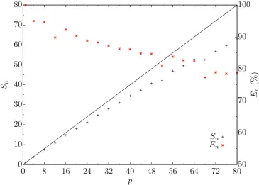
1.1 ABABAB stacking layers for ice-Ih (left) and ABCABC stacking lay-ers for ice-Ic (right). The normal of both the ice-Ih (basal) and ice-Ic (111) plane, is parallel to the length of the page. . . 3 2.1 Speedup test of LAMMPS mW liquid simulation using 21,952

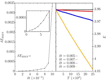
par-ticles. Black data points indicate the actual speedup fraction of the simulation, compared to perfect speedup shown by the black line. Red points indicate the efficiency of actual speedup compared with the theoretical maximum speedup for the number of processors used. 22 2.2 The RMS deviation in total energy with varying timestep (left) and

the total energy as a function of simulation time for different timesteps (right). These results are for an 864 atom, liquid simulation atP∗= 0, T∗ = 0.7, within the NVE ensemble, using the modified LJ-BG potential described in section 2.7.1. All values are in LJ reduced units for=σ = 1. . . 25 2.3 Equilibration of total energy (E), temperature (T) and pressure (P)

in a LJ solid-liquid coexistence MD simulation for the (100)[001] ori-entation. The timestep for the simulation is δt = 0.005 and the sampling is every 100 steps. All values are in LJ reduced units for

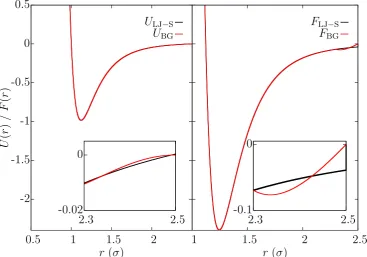
=σ = 1. . . 26 2.4 The form of the potentials (left) and force fields (right) for the shifted

LJ potential (black) and the LJ-BG potential (red). The inserts show the detail in the tails for 2.3σ ≤ r ≤ 2.5σ. Both potentials have

= σ = 1 and the form of the shifted LJ potential is ULJ-S(r) =

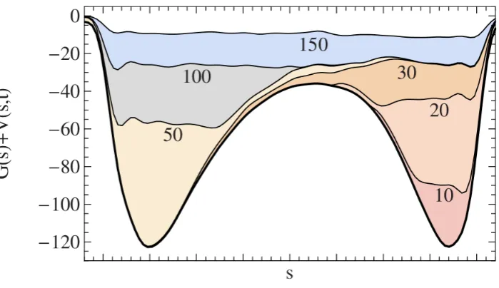
3.1 Illustration of a metadynamics algorithm exploring the free energy hypersurface; taken from ref. [56]. The underlying free energy hyper-surface is shown as a function of reaction coordinate s, G(s), given by the solid black curve. The accumulated biasing potential,V(s), is shown at different times, denoted by different colours. . . 39 4.1 Simulation profile for the (111)[1¯10] system using the q12 order

pa-rameter and 80×1×50 bins in thex,yand zdirections respectively. The red points indicate the average position of the interface detected alongx in a region of size ∆z along z. . . 45 4.2 q12 order parameter profile and fit during an LJ-BG simulation of the

(100)[001] orientation, without discretisation in x, (left), and when using a discretisation of 100×50 bins in thexz plane, (right). . . . 51 4.3 Log-log plots of the interfacial stiffness for LJ-BG systems after using

theq12 order parameter. . . 56 4.4 Left: Fitted interfacial stiffness values for the LJ (100)[001]

orienta-tion up to and including N wavenumbers. Right: The measured χ2

and R2 _{values for the fit up to differentN wavenumbers. . . . 58}

4.5 Exponential dependence of the autocorrelation function for

|h(q)|2

in the (100)[001] LJ-BG system for varying values ofq. . . 60 5.1 RDF plots for the three bulk solid-phase ice systems in the mW

model: ice-Ic (left), ice-Ih (centre), ice-0 (right). . . 66 5.2 For ice-Ic and water, using an order parameter cutoff of 3.5 ˚A, the

plot shows: (left) the q6 correlation distribution; (centre) the num-ber of neighbours; (right) the number of solid-like bonds when using

c(i, j)≥0.5 and 4 neighbours. . . 68 5.3 Theq6 bond correlation distribution in ice-Ih and water over 3.5 ˚A. 69 5.4 The number of solid-like bonds in ice-Ih and water over 3.5 ˚A when

nearest neighbours = 4 andc(i, j)≥0.25 (left) or c(i, j)≥0.5 (right). 70 5.5 Theq6 bond correlation distributions in ice-0 and water over the first

coordination shell (left) and the second coordination shell (right). . . 71 5.6 The q3 bond correlation distribution in ice-Ic and water (left) and

ice-Ih and water (right), over an order parameter cutoff of 3.5 ˚A. . . 73 5.7 q3 bond types in liquid (black lines) and solid ice-I (red lines). Solid

5.8 Theq3 bond correlation distributions in ice-0 and water over the first coordination shell (left) and second coordination shell (right). . . 74 5.9 The q3 order parameter profile in ice-Ic (111)[1¯10] simulation using

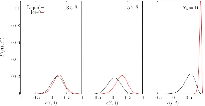
different assigned order parameter values to identify solid, interface and liquid particles. The vertical line is the average position of the two inflexion points (x= 202.694 ˚A). . . 76 5.10 The q12 bond correlation distribution in ice-0 and water over 3.5 ˚A

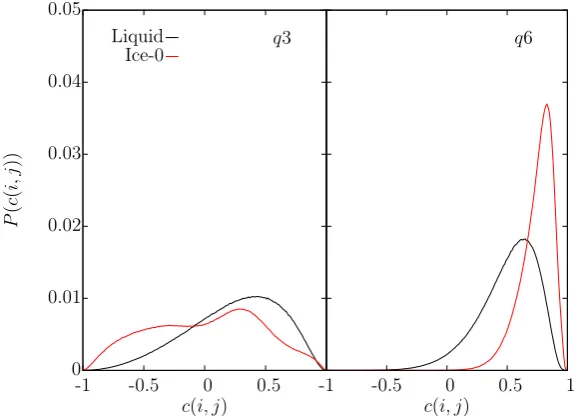
(left), 5.2 ˚A (centre) and when spatially averaging over the nearest 16 neighbours (right). . . 77 5.11 The spatially averaged bond correlation distribution in ice-0 and

wa-ter over the 16 nearest neighbour atoms for q3 (left) and q6 (right). 78 5.12 The q12 correlation distributions in ice-Ic and water over the first

coordination shell (left) and spatially averaging over the 16 nearest neighbours (right). . . 79 5.13 The q12 correlation distributions in ice-Ih and water over the first

coordination shell (left) and spatially averaging over the 16 nearest neighbours (right). . . 80 5.14 The number of solid-like bonds in ice-Ic (left), ice-Ih (centre) and

ice-0 (right) against water when c(i, j) ≥ 0.75 and q12 is spatially averaged. . . 80 5.15 Maps of the (basal)[11¯20] interface in ice-Ih with varying length in y

and the RMS displacement plots along the interface. Bin widths are approximately 3.6 ˚A in both (a) and (b). . . 82 5.16 Measured interfacial stiffness for simulations of various short direction

lengths, y, and number of bins along z, nz, for the (basal)[11¯20]

simulation. 80 bins are used along the long direction and q12 has been used to identify the interface. . . 84 5.17 Measured interfacial stiffness for various bins in the long direction

of the system, for one orientation in each of the ice structures. The number of bins along the interface is kept constant with 50, 50 and 100 bins, respectively. . . 85 5.18 Measured interfacial stiffness for varying number of bins across z in

simulations of the different ice structures. 80 bins are used along the long direction of the simulation in all cases. . . 87 5.19 As figure 5.18, but with varying the maximum value of qz used,

5.20 The coordinate system used (left) forms an orthogonal set of unit vectors from the SASH coordinates whereer is always normal to the

interface; demonstrated in the (111)[1¯10] simulation (right). . . 91 5.21 The ice-Ic (top row), ice-Ih (middle row) and ice-0 (bottom row)

crystal unit cells and planes. The SASH basis coordinate system axes are shows in blue and the crystal cell axes are shown in red, on the unit cells, while the local simulation axes are shown in black on each of the planar images. The construction of each cell is given in (a b c α β γ) notation[87]: ice-Ic (1 1 1 π/2 π/2 π/2); ice-Ih (1 1 1.630π/2π/2 2π/3); ice-0 (5.905 5.905 10.674π/2π/2π/2). . . 92 6.1 Measured interfacial stiffness for orientations in each of the ice

struc-tures against production run time. . . 102 6.2 Temperature of solid region and percentage of solid in ice-0 (001)[010]

simulation over the 5 ns equilibration period, sampling every 1 ps. . 104 6.3 Interfacial stiffness plots for ice-Ic at various interfaces using theq12

order parameter and analysis geometry as specified in table 6.2. . . . 107 6.4 Interfacial stiffness plots for ice-Ih at various interfaces using theq12

order parameter and analysis geometry as specified in table 6.2. . . . 109 6.5 Interfacial stiffness plots for ice-0 of various interfaces using the q12

order parameter and analysis geometries as specified in table 6.2. . . 111 6.6 Interfacial stiffness plot for ice-Ic (111)[1¯10] orientation using theq12

order parameter. The fits have been performed with: ˜γonly, shown in red; with ˜γ and the elastic modulus (E =−0.14(14) mJ m−3_{), shown}

in black; and also with ˜γ and the bending rigidity (κ= 242(20) mJ), shown in blue. . . 112 6.7 Fit lines for calculatedγ0Ice-0 and γ0Ice-Ih and the extracted trend for

γ0Ice-Ih from Espinosa et al. Data points are also extracted from the

work by Espinosa et al. but were originally produced by Limmer and Chandler[98] and Li et al.[6]. . . 118 6.8 Measured versus fitted interfacial stiffness results for the three

6.9 Polar plot for ice-Ic interfacial stiffness using 3, 4 or 5 fitting param-eters; shown blue, black and red respectively. The plot shows the measured values of the interfacial stiffness, usingq12, alongu= [1,0] at φ= π/4. Note that the (001) is symmetrically equivalent to the (100) plane. . . 120 6.10 Polar plot for the ice-0 interfacial stiffness alongu = [1,0] at φ= 0,

with measured stiffnesses usingq12. . . 120 6.11 The P-T phase diagram of mW water, reproduced from ref. [17].

The solid lines demonstrate coexistence between liquid and ice-Ih/Ic (blue), and liquid and ice-0 (red). The dashed lines are constant chemical potential differences between liquid and ice-Ih/Ic (blue), and liquid and ice-0 (red). The red open circles indicate homoge-neous nucleation of ice-0. The reader should refer to ref. [17] for a comprehensive description of the additional (green) information. . . 124 7.1 Interface growth rates (black) for an initial ice-Ih (basal) interface

at various degrees of supercooling below the average melting tem-perature, Tm = 277.09(3) K, and 1 atm. Also shown is the relative

percentage of ice-Ic (red) in the newly formed solid region at the end of the simulations. . . 127 7.2 Initially a 1:1 system of ice-Ih and water, with a (basal) plane

in-terface. This figure shows the newly formed ice-Ih (grey) and ice-Ic (orange) particles after a simulation of 5 ns at 8 K below Tm. Also

present are interface (red) and water (blue) particles, as identified by

q3. The region “R”, is the original section of ice-Ih. . . 128 7.3 Result of the autocorrelation function for∂γG(λ0) against MC sweeps,

sampling every 10 sweeps over a total of 1×106 in ice-Ih. The red line is a fit of exp(−n/τ). . . 137 7.4 Quantities for the mW model at different parameter sets, λ0, for

varying δ. Top: The result of equation (7.23). Upper middle: The melting temperature of ice-Ih obtained from coexistence MD simu-lations. Lower middle: The density of ice-Ih obtained from the MC simulations. Bottom: The Gibbs free energy gap as calculated by equation (7.22), plus the initial gap. . . 140 C.1 Plots of the SASH equations for ice-Ic representing the free energy

and the interfacial stiffness with unit vectors u =eθ and u =eφ as

C.2 Plots of the SASH equations for ice-Ih representing the free energy and the interfacial stiffness with unit vectors u =eθ and u =eφ as

shown. . . 152 C.3 Plots of the SASH equations for ice-0 representing the free energy

and the interfacial stiffness with unit vectors u =eθ and u =eφ as

Acknowledgements

First and foremost, I would like to thank my supervisor, Dr David Quigley, for all his advice and guidance over the last four years. Without his support, I would most likely not have begun this work, let alone finished. I would also like to extend my thanks to Prof. Mike Allen, who encouraged me throughout the first several months of this project, and to both Prof. George Rowlands and Dr Bart Vorselaars, who graciously provided help when needed.

I would also like to personally thank the many people I’ve met during my time at Warwick. It’s true that the people make the place, which in turn shapes you. I am extremely grateful for all the experiences I have had during this project; it has been richly rewarding.

To my office mates over the years, I would particularly like to thank Dr Anja Humpert, Dr Gil Rutter, Dr Sally Bridgwater and Dr Sam Brown, who each provided the moral support that only fellow Ph.D. students can; and in one case, a much needed change of perspective.

I would like to thank all of WUSAC for giving me some amazing experiences from around the world. The time I shared with you all allowed me to return to my work refreshed and ready. I would especially like to thank Francesca Parker, Andy Loo, Eleanor Kelly, James Christen, Dr Francesco Fermani, Emma Orton and Heather Barnes; you made WUSAC what it was for me.

To my housemates over the years, particularly Kateryna Taylor, Cyril Chimisov, Adam Griffin and Ting Chen, I thank you for being there and making my house feel like a home.

advice and some great food! You made things just a little bit easier.

Joe and Sam Rearden: I’ve never met two people who are more affirmative and optimistic. You are both a real inspiration for my determination to keep going. I would also like to thank many friends from before Warwick, for all their support in one way or another; especially Dr Jonathan Watkins, who has always been an inspiration.

To Eleanor O’Shea, I am truly thankful for the stability you have provided me with and the clarity of mind I needed to get this work completed.

Declarations

This thesis is submitted to the University of Warwick in support of my application for the degree of Doctor of Philosophy. It has been composed by myself and has not been submitted in any previous application for any degree.

The work presented (including data generated and data analysis) was carried out by the author except in the cases outlined below:

Abstract

This research applies the capillary wave method (CWM) to quasi-2D systems in order to calculate the solid-liquid coexistence interfacial free energy (γ) of ice-Ic, ice-Ih and ice-0, with water, at 1 atm, within molecular dynamics simulations employing the coarse-grained monatomic water (mW) model. Investigations are performed to determine how the measured interfacial stiffness (˜γ) is affected using various: i) order parameters, to distinguish between the solid and the liquid; ii) analysis discretisation, for interface profiling; iii) system thicknesses.

The values ofγ for the different crystal planes (γplane) shows that for ice-Ih

γbasal < γprism . γ11¯20, for ice-Ic γ111 . γ112 . γ110 < γ100 and for ice-0 γ001 <

γ102 . γ110 . γ101 . γ100. It is also found that between ice-Ic and ice-Ih, γ110 ≈

γ_11¯20 and γbasal ≈γ111 to 0.3 mJ m−2 outside of errors. All structures are weakly

anisotropic in γ compared to their ˜γ, with ice-Ic, ice-Ih and ice-0 having ranges of 1.5(4), 2.5(5) and 3.9(7) mJ m−2, respectively, between their measured planes. The isotropic component ofγ for the different structures (γ0Structure) shows γ0Ice-0 =

33.8(4),γ0Ice-Ih = 36.0(3) and γ0Ice-Ic = 36.3(3) mJ m −2_.

The rationality that ice-I nucleation can be catalysed at strong supercooling within a shell of ice-0 is explored. It is found that at 215.2 K such nucleation could occur, forming an ice-0 shell of 3.3 ˚A thick around a core of ice-Ih.

Chapter 1

Introduction

1.1

Motivation

Calculating the interfacial free energy between a crystal and its melt is necessary to properly understand the behaviour of crystal nucleation. On a microscopic scale, the magnitude of the interfacial free energy strongly controls the growth rate, while the anisotropy determines the dendritic growth and morphology of the crystal[1]. Knowledge of the anisotropy is particularly important for being able to reliably perform nucleation calculations which often assume a spherical symmetry of the interfacial free energy. Hence, if there is significant anisotropy present, such calcu-lations are invalid[2].

Practically, being able to control the dendritic growth grants control over the formation of crystal microstructures, which appear as a crystal solidifies[3]. This can be used in metallurgy to create stronger alloys and metals, where, for example, the material sheer stress is inversely correlated to the size of grains within the material[4]. Interfacial free energy calculations are also important in studying ice nucleation in clouds, determining whether nucleation begins within or on the surface of such water droplets, and the subsequent effect this has on crystallisation rates in the presence of other aerosols in the atmosphere[5, 6]. This has direct implications on constructing more accurate climate models, since the radiative properties of cirrus clouds are dependent on the morphology, concentration, distribution and growth rates of the ice crystals within them[7, 8].

on the type of ice nuclei precursor[10]. Hence, by knowing the value for the inter-facial and bulk free energy of different ice structures, the preferential structure for nucleation can be determined at a specific temperature and pressure. This is useful in the development of solvents to stop these preferential ice nuclei from forming, which is applicable to: cryogenic storage of tissues, to stop ice from destroying cells; and antifreeze agents, to stop ice build up on aircraft wings[11].

However, in general, experimental measurement of the anisotropy of the in-terfacial free energy is difficult in systems with weak anisotropy[12]. Experiments that rely on measuring the interfacial free energy from classical nucleation theory, yield only averaged interfacial dependence and are typically 10-20% lower in their estimates than reality, while experiments that rely on contact angles do not usually have the precision to resolve the anisotropy[1]. Indeed, there are only a few excep-tions where the anisotropy of the free energy has been directly measured, limited to transparent organic systems[13]. Of these, only one experiment has managed to measure the anisotropy in ice via measuring contact angles of water in an ice-I ma-trix at atmospheric pressure, which revealed the (basal) plane to have a much lower degree of anisotropy than that of the edge planes[14]. Such experimental difficulties and low sensitivity to the anisotropy, provides the necessity to turn to computational methods to more accurately measure the interfacial free energy and its anisotropy.

In order to use computational methods effectively, it is of crucial importance that the model potentials used, accurately reproduce experimentally observed re-sults. Models that yield results to the contrary, cannot be used to make accurate conclusions about the nature of reality. Sufficient effort should therefore be given to developing more accurate models, and to establishing the limitations of such models, to avoid making false claims about reality.

1.1.1 Ice-I

As discussed above, ice nucleation has relevance to the integrity of many kinds of systems, from climate models to mitigating cell damage. The ice being referred to in these terrestrial systems is ice-I. However, there are at least 15 crystalline phases of ice – excluding amorphous phases – currently known, that make up the rich phase diagram of water[15]. This research is concerned with the formation of ice at atmospheric pressure at coexistence with liquid, and so only ice-I need be considered out of the existing 15 phases. Yet, ice-I itself is a richly complicated phase of ice, which may exist as one of two polytypes: hexagonal ice-I (ice-Ih) and cubic ice-I (ice-Ic)[15].

atmo-Figure 1.1: ABABAB stacking layers for ice-Ih (left) and ABCABC stacking layers for ice-Ic (right). The normal of both the ice-Ih (basal) and ice-Ic (111) plane, is parallel to the length of the page.

spheric pressure from 73 K to 273.15 K[15]. The stable form of ice-I is ice-Ih, which is observed experimentally in a pure state at temperatures T > 263 K[16]. At lower temperatures, nucleation of ice-I has been observed to form metastable ice-Ic precursor nuclei to that of ice-Ih[16]. The difference between these two polytypes is that of the stacking order in only one direction of the crystal structure. Ice-Ih follows a repeating ABABAB stacking pattern in the direction of the normal of the (basal) plane, while ice-Ic follows an ABCABC stacking pattern in the direction of the normal of the (111) plane, as shown in figure 1.1; additionally, diagrams of the crystal cells are found in chapter 5.

Unlike ice-Ih, pure ice-Ic has never actually been observed experimentally. Instead, there is increasing evidence from neutron diffraction patterns to suggest that metastable ice-Ic is actually stacking disordered ice-I (ice-Isd), consisting of random arrangements of cubic and hexagonal ice-I planes[16]. It also transpires that the quantity of ice-Ic present in ice-Isd is temperature dependent, with increasing cubicity with decreasing temperature to approximately 50% cubicity[15, 16]. This is discussed in much greater detail in chapter 7, but it is worth noting that given ice-Isd – rather than pure ice-Ic – may actually nucleate as a precursor to pure ice-Ih, means that calculated and reported differences between the free energies of ice-Ih and pure ice-Ic, are extrema, rather than reflecting actual experimental conditions.

1.1.2 Ice-0

ice-0 is predicted to form at T ≤ 245 K; as researched in chapter 6. Under such conditions, ice-0 has a structure that is more similar to that of the liquid than that of ice-Ic or ice-Ih, consisting of tetragonal ordering[17]. Such microscopic similarity to the liquid structure results in a comparatively lower interfacial free energy barrier with that of water, than that of an ice-Ic and water or ice-Ih and water; making homogeneous nucleation of ice-0 favourable. The formation of ice-0 nuclei therefore act as nucleation points for catalysing heterogeneous nucleation of more stable ice-I nuclei, which have similar interfacial free energies with that of ice-0 than with that of the liquid, as predicted by Ostwald’s step rule[18]. This is discussed in greater detail in chapters 3 and 6. The unit cell for ice-0 can also be found in chapter 5.

Calculating the solid-liquid interfacial free energies of ice-I and ice-0 crystal systems can help answer questions about how ice nucleates at atmospheric pressures and whether ice-0 has a role in the formation of ice-I[17, 19]. If ice-0 does indeed have an influence in nucleation, this could have wider consequences – as previously mentioned – on accounting for changes in the radiative properties of ice crystals forming in clouds, impacting climate models, or motivating the development of more sophisticated antifreeze agents for operation in extreme environments.

1.2

This Research

This work focuses on the use of the capillary wave method (CWM), to calculate the interfacial free energy of ice-Ic, ice-Ih and ice-0 in contact with water at atmo-spheric pressure, using the coarse-grained monatomic water (mW) model established by Molinero and Moore[20], through the use of molecular dynamics (MD) simula-tions. While there are several computational methods that exist to calculate the interfacial free energy and its anisotropy, each method has its own advantages and disadvantages. A review of such methods is conducted in chapter 3, along with a discussion regarding nucleation theory and the nucleation of the ice structures studied in this research.

Before a review of nucleation and free energy methods, the theoretical back-ground for numerical simulations, practicalities and statistical physics are first dis-cussed in detail in chapter 2; upon which this work is heavily dependent. Chapter 2 also reviews the model potentials used in this research. Following, chapters 2 and 3, this thesis begins to describe the research conducted in earnest.

results against those in the literature for the same planar interface orientations of a simple face centred cubic lattice interacting in a Lennard-Jones type potential.

Chapter 5 then discusses how to distinguish between solid-like and liquid-like particles in ice, the choice of interface analysis parameters and how to use spherical harmonics to describe the form of the interfacial free energy. The methods developed in chapters 4 and 5 are then applied to various ice-Ic, ice-Ih and ice-0 systems to calculate the interfacial free energy; the results of which are presented and discussed in chapter 6.

Chapter 2

Theoretical Background

2.1

Introduction

The main research conducted in this thesis relies heavily on concepts from statistical physics and scientific computing, aspects of which are discussed here. This chapter begins with a review of ensembles in the context of statistical physics. Following, is a discussion of the principles of molecular dynamics, along with the use of barostating and thermostating, and also performing Monte Carlo simulations. The chapter then covers the practicalities involved with molecular dynamics simulations, before finally covering the model potentials used in the work.

2.2

Ensembles

For a thermodynamic system ofN particles, macroscopic quantities such as energy, temperature and pressure, are observed. Such a system evolves classically accord-ing to Hamilton’s equations of motion and in statistical physics, these macroscopic quantities can be related to the microscopic quantities of position and momentum of each particle in the system. This follows from the Virial theorem[22]

xi

∂H

∂xj

=kBT δij, (2.1)

wherexiis a particle’s position or momentum. For example, the temperature of the

system can be given by the average kinetic energy of all the particles at that point in time,

p2_i

2m

= ν

whereν is the number of degrees of freedom per particle and pi is theith particle’s

momentum. Therefore, if the “microstate”, which is the complete microscopic de-scription of all particles’ position and momenta at timet, can be calculated, then it is also possible to calculate all macroscopic quantities of the system att. The set of macroscopic observables that a system has is called the “macrostate” and there may be many unique individual microstates that describe a single macrostate. Further-more, there may be many systems, each in a unique microstate, that when evolved in time yield unique trajectories from one microstate to the next, but where the average of one trajectory is equivalent to that the other systems’ and all still yield the same macrostate. The collection of such systems is called an “ensemble”[22].

The ensemble exists in a domain known as “phase space”. The phase space is a 2dN dimensional space – where d is the dimensionality of a system in real space – which describes all the possible microstates that a system ofN particles can access. The dimensionality of the phase space is such, due to N particles having d

dimensional descriptions of position and momentum. This results in each microstate being described by a unique phase space coordinate: x = {r1, ...,rN,p1, ...,pN}.

However, if a system is described by some ensemble, then the system must have a well defined macrostate. This restricts the accessible microstates of a system’s trajectory to within a bound hypervolume of the phase space. Since on average a trajectory will produce the defined macrostate, the microstates are accessible according to the ensemble probability distribution. For example, a finite number of equally accessible microstates exist on a constant energy hypersurface, but this is only true for systems described exactly by Hamilton’s equations of motion, since these are energy preserving[22]; see section 2.2.1.

The description of an ensemble implies that it is not necessary to calculate the exact equations of motion for every particle in the system at every instant in time in order to observe the macroscopic properties of the system. Instead, with access to the entire ensemble describing the macrostate of interest, the observables can be recovered from averaging the microscopic description of the observable over the ensemble by the number of microstates that describes the ensemble. Mathematically, this is

A= 1

Z

Z

dxa(x)F(H(x)), (2.3)

where a(x) is the function giving the microscopic description of the observable A,

Calculation of equation (2.3) is not typically possible analytically. Instead, numerical techniques are required such as molecular dynamics (MD), which is dis-cussed further in section 2.3. Using a technique such as MD, allows the system to evolve from a single microstate and explore the ensemble phase space hypervolume. For equilibrium systems, given infinite time the system will visit each microstate within the hypervolume, which assumes the system is “ergodic”. Recording the full evolution of the system over time allows the full recovery of the ensemble, and thus measurement of the necessary macroscopic observable. Hence, to measure any observable, the relevant partition function, Hamiltonian and Virial must be known. The Hamiltonian for each of the ensembles depends upon the type of thermostat or barostat being used in the simulation. As such, these Hamiltonians are discussed in section 2.4.

Ergodicity is an important requirement of the evolution of an ensemble if correct sampling via MD is to be obtained. If a system is not ergodic, then it is not possible to positively state that the MD simulation is sampling the correct ensemble. For a system to be considered ergodic requires: sampling be done at time intervals longer than the longest correlations; the integration scheme to be phase space area preserving, i.e. “symplectic”; and the simulation duration to be long enough that it reproduces the ensemble probability density function[23]. Ergodic processes are time reversible and therefore allow ensemble averaging to be done at any time once the phase space has been thoroughly explored.

There are many ensembles that MD simulations can be used to recover. A brief description of each of the ensembles used throughout this research, follows.

2.2.1 Microcanonical (NVE)

Simulating an isolated system for a constant number of particles,N, over a constant volume, V, and energy, E, generates the microcanonical ensemble. This ensemble follows Hamilton’s equations of motion exactly and therefore the Hamiltonian that describes such a system is just[22]H(x) =E. The partition function for the micro-canonical ensemble is therefore[22]

Ω(N, V, E) = E0

N!h3N

Z

dxδ(H(x)−E), (2.4)

where E is the fixed total energy of the system, E0 is a small energy shell above

the constant energy hypersurface andhis Planck’s constant. The constantsE0 and

respec-tively. It should be further observed that the uncertainty of the phase space vector ∆x ≡ (∆x)3N(∆p)3N = h3N, from Heisenberg’s uncertainty principle. The factor

N!, compensates for overcounting, since classically the particles are distinguishable. Since the energy is fixed, this has the effect of fixing the phase space hypersurface and so a simulation can only explore the states within this ensemble with equal probability.

2.2.2 Canonical (NVT)

The microcanonical ensemble generates conditions that are not representative of actual experimental conditions. In reality, the total energy is not fixed but rather other thermodynamic quantities. The canonical ensemble is an example of a such a system, which fixes the number of particles N, the volume of the system V, and fixes the temperature of the systemT, to an infinite heat bath. Given that such a system is in contact with a heat bath, the energy can fluctuate as to maintain a fixed temperature. This means the Hamiltonian of the system is not conserved. Instead, the system exists on a constant “Helmholtz free energy” hypersurface;F =E−T S.

The partition function that describes such an ensemble is

Q(N, V, T) = 1

N!h3N

Z

dxexp[−βH(x)], (2.5)

where the Hamiltonian follows a Boltzmann distribution.

Normally, experiments are carried out under constant pressure rather than constant volume. An alternative ensemble is the isobaric-isothermal ensemble, dis-cussed in section 2.2.4. However, in the limit of large enough systems, the canonical ensemble actually approximates to the isobaric-isothermal ensemble.

2.2.3 Isobaric-Isoenthalpic (NPH)

Instead of fixing the temperature of the system, it is instead possible to fix the pressure of the system. This leads to the development of an ensemble with constant particles N, pressure P and, by extension, enthalpy H = E +P V. Coupling the system to an external piston, allows the volume to fluctuate so that the average internal pressure is fixed. This generates the isobaric-isoenthalpic, or NPH, ensem-ble and the system evolves under Hamilton’s equations across a constant enthalpy hypersurface.

with the partition function

Γ(N, P, H) = H0

V0N!h3N

Z ∞

0

dV

Z

dxδ(H(x) +P V −H). (2.6)

The partition function is now also dependent on the volume, as the position of each particle is dependent on the number of positions available to it within the volume of the system.

2.2.4 Isobaric-Isothermal (NPT)

Experiments normally report macroscopic observables for systems ofN particles un-der conditions of constant pressure,P, and temperature,T. Therefore, the isobaric-isothermal, or NPT, ensemble is necessary to use to compare simulated conditions to those of actual experiments. The NPT ensemble extends the canonical ensemble, coupling the system to both an external heat bath and an external piston. With the inclusion of pressure, the system now exists on a constant “Gibbs free energy” hypersurface,G=E−T S+P V.

The partition function for the NPT ensemble is

∆(N, P, T) = 1

V0N!h3N

Z ∞

0

dV

Z

dxexp[−β(H(x) +P V)]. (2.7)

2.3

Molecular Dynamics Techniques

In principle, a MD simulation is just a virtual collection of particles constrained to behave according to some defined parameters and allowed to evolve in time[22, 24]. Some thermodynamic properties can be extracted from the system as it evolves, while others have to be measured over the duration of the simulation such as the change in the free energy between two states and entropy[24]. The latter case is due to the fact that these quantities are dependent on the partition function of the system, rather than an actual instantaneous physical property. As such, the change in the free energy must be computed via thermodynamic integration over the thermodynamic path between the system’s initial and final state. Since the former case is concerned with instantaneous properties of the system, these quantities can be extracted through the use of the Virial theorem[22].

The basic procedure for an MD simulation is as follows[24]:

• The system is evolved over a predetermined number of iterations.

• Each iteration requires the forces between each pair of particles to be calcu-lated, subject to the potential being used, as well as the present positions of each particle.

• Once force calculations have been performed, the equations of motion must be integrated to acquire the next set of particle positions for the next iteration.

• Averages of microscopic properties, such as kinetic energy, can be taken to obtain thermodynamic properties.

• Iterate to the next timestep.

• The simulation terminates once the maximum number of iterations has been reached.

There are many different types of algorithms that exist to perform the simulations, however one of the most widely used and stable is the Verlet algorithm[24].

2.3.1 Verlet Algorithm

The Verlet algorithm is used to compute the next particle positions from the present particle positions, previous particle positions and the forces between the particles[25]. Since it depends on the previous particle location, it is necessary to prepare a fic-tional previous state at the very beginning of the simulation.

At the beginning of the simulation, the initial state is prepared according to a set of defined conditions. The system can be initialised in a well defined ordered state, such as a solid crystal lattice with all particles at their lattice sites. Liquid systems can then be set up by melting the structure over the equilibration period before performing statistical sampling. It is also important that no particle positions overlap with each other, as this would yield non-physical results; such as highly repulsive forces between particles causing rapid changes in the total energy of the system and explosion of the simulation volume. Particles are then each assigned a velocity, v, sampled from a distribution and scaled so that the centre of mass momentum is zero. In order to obtain the fictional previous state, the system is run backwards in time for a very short timestep, dt, so that all particles move a distance −vdt. The program then has access to a set of previous particle locations and present particle locations with which to iterate to the next set timestep.

costly part of the program, since forN particles it requires looping overN(N−1)/2 unique particle pairs in the system and computing the total force on a particle from each of its neighbours. This is an orderN2_{calculation and therefore extremely slow}

for large systems. The calculation can be performed over fewer pairs by considering the form of the particle potential used in the system. If the potential and force fields are close to zero at some radius away from each particle, as demonstrated in section 2.7, then the calculation only needs to be performed for particle pairs within that radius for each atom.

The calculation itself is simply,

f(r) =−∇U(r), (2.8) wheref(r) is the force in the vector spacerandU(r) is the potential in vector space

r. The Verlet algorithm uses a Taylor expansion about the forward time increment, ∆t, in position,

r(t+ ∆t) =r(t) + ˙r(t)∆t+¨r(t)∆t

2

2 + ...

r(t)∆t3

3! +O(∆t

4_{), (2.9)}

and, symmetrically, the backward time increment,

r(t−∆t) =r(t)−r˙(t)∆t+¨r(t)∆t

2

2 − ...

r(t)∆t3

3! +O(∆t

4_{). (2.10)}

Simply adding equations (2.9) and (2.10) together and rearranging for the forward time increment gives the Verlet algorithm:

r(t+ ∆t) = 2r(t)−r(t−∆t) +f(t)∆t

2

m +O(∆t

4_{). (2.11)}

total number of calculations that need to be performed for the same total duration of the simulation. However, there are two further aspects that need to be considered. These aspects are long-term energy drift, since the equations of motion are energy conserving, and “Lyapunov instability”[24].

Lyapunov instability describes how the trajectory of the system across a phase space hypersurface, for constant energy, will diverge exponentially from the true trajectory of the system. This is actually not that problematic as MD simu-lations are not concerned with exact simusimu-lations of systems, but rather statistical results[22]. Furthermore, evidence suggests the existence of “shadow orbits”, which are true trajectories of the system that closely track the computed trajectory of the system, for durations longer than the Lyapunov instability[24, 26]. This implies the computed trajectory does actually match a true trajectory that exists within the system.

Therefore, the more important aspect to consider is whether the system is phase space volume preserving; i.e. the system has access to the same microstates on the constant energy hypersurface, indicating no long-term energy drift in agreement with Hamilton’s equations of motion[22]. Algorithms that suffer from this heavily are those that are not time reversible. Despite the time reversibility of the Verlet algorithm, it does not conserve the total energy exactly. Instead it conserves a “shadow” Hamiltonian that tends to the true Hamiltonian with decreasing timestep size[22, 24]. Higher order Verlet-like algorithms do a much better job at accurately following the true trajectory of the system over short timescales, but are much poorer at preventing long-term energy drift[24]. This makes low order, short timestep, Verlet algorithms suitable for long duration MD simulations.

2.4

Barostats and Thermostats

Using MD to sample the desired ensemble requires using the correct equations of motion and Hamiltonian that describes the entire system. As mentioned in section 2.2, integrating Hamilton’s equations of motion to iterate the MD simulations re-produces the microcanonical ensemble. If one wishes to use MD to sample other ensembles, then Hamilton’s equations of motion can not be used directly. Further-more the simple Hamiltonian defines a constant energy hypersurface, while the other ensembles conserve different hypersurfaces in phase space and the energy fluctuates about an average due to interactions of the system with its environment.

size of their container, such as systems in the NPH ensemble, are controlled by a barostat. These additional controls enter as separate degrees of freedom into the Hamiltonian, and are discussed in sections 2.4.1 and 2.4.2 respectively. The NPT ensemble relies on both a thermostat and barostat and is discussed at the end of section 2.4.2.

2.4.1 Thermostats

The simplest way to control the temperature of the system is to rescale the velocities so the kinetic energy generates the required temperature instantaneously. This procedure lead to the development of the Nos´e Hamiltonian[27]

H_N=

N

X

i=1

p2_i

2mis2

+U(r1, ...,rN) +

p2_s

2Q + (dN + 1)kBTlns , (2.12)

where s is a separate entity that scales the instantaneous kinetic energy, ps is the

conjugate momentum tosand Qacts as a fictional mass term effecting how rapidly the kinetic energy is rescaled in the response to thermal fluctuations; the actual dimensionality ofQ is energy×time2. This generates a canonical partition function with the following equations of motion:

˙

ri =

∂H_N

∂p_i = p_i

mis2

˙

p_i =−∂HN

∂ri

=fi

˙

s= ∂HN

∂ps

= ps

Q

˙

ps=−

∂H_N

∂s = 1 s "_N X i=1

p2_i

mis2

−(dN+ 1)kBT #

. (2.13)

The equations of motion associated with the Nos´e Hamiltonian actually act upon a non-standard form of the kinetic energy, as shown in equation (2.12). Thefore, to recover the actual kinetic energy, a noncanonical change of variables is re-quired by transforming, p0_i = p_i/s, p_s0 = ps/s and dt0 = dt/s. However, making

such a change of variables results in the equations of motion no longer being sym-plectic, which, as previously mentioned, is a requirement for correct sampling of the ensemble.

Nos´e-Hoover equations of motion of the form: ˙

ri =

p_i

mi

˙

p_i =fi−ζpi

˙

ζ = 1

Q

" _N X

i=1

p2_i

mi

−dN kBT #

, (2.14)

where the quantity dN + 1 has also been redefined as dN. The term ζ ≡ ps/Q

is described as a “frictional” term by Hoover, which determines how rapidly the temperature of the system adjusts. The Nos´e-Hoover equations generate a canonical distribution in an ergodic system, but does not necessarily sample the canonical ensemble properly for a non-ergodic system. Hoover showed that for a harmonic oscillator the phase space was not properly sampled due to the system not being sufficiently chaotic. One reason for this was suggested by Martyna et al.[29], which indicated that the distribution in phase space has a Gaussian dependence on pi

but also on the thermostat momenta. In the Nos´e-Hoover equations, the momenta of the particles is controlled by the thermostat, but there is no fluctuation of the thermostat momenta. For the system to be truly ergodic, the thermostat momenta should also be explored across the phase space.

M as presented by Martyna et al.[29]: ˙

ri=

p_i

mi

˙

p_i=fi−

pη1

Q1

p_i

˙

ηj =

pηj

Qj

j= 1, ..., M

˙

pη1 =

"_N X

i=1

p2_i

mi

−dN kBT #

−pη2

Q2

pη1

˙

pηj =

"

p2 ηj−1

Qj−1

−kBT #

−pηj+1

Qj+1

pηj j = 2, ..., M−1

˙

pηM =

"

p2_ηM−1 QM−1

−kBT #

. (2.15)

2.4.2 Barostats

In order to control the pressure of the system, the volume must be allowed to fluctuate. A simple method analogous to rescaling the kinetic energy to control the system temperature was first proposed by Andersen[30], which involves scaling the position and momenta of each particle by the volume of the system; si = V−1/3ri

andπi =V1/3pi, respectively. This introduces the volume explicitly as a dynamical

variable into the phase space domain, with conjugate momentumpV. This leads to

the construction of Andersen’s Hamiltonian for isobaric-isoenthalpic systems[22]

HA= N

X

i=1

V−2/3π2_i

2mi

+U(V1/3s1, ..., V1/3sN) +

p2 V

2W +P V , (2.16)

where the termP V describes the action of an imaginary external piston regulating the volume in response to fluctuations of the internal pressure about that of the external applied pressure P. The term p2_V/2W, acts as the kinetic energy of the volume with fictional massW controlling the responsiveness of the external piston to changes in the internal pressure; increasing the mass has the effect of damping the piston. The fictional mass has the form W = (3N + 1)kBT τ2, where τ is the

timescale of the volume fluctuation.

Applying Hamilton’s equations of motion results in the Andersen equations of motion for the isobaric-isoenthalpic ensemble in terms of ˙siand ˙πi. These equations

can be transformed in terms of the physical coordinates ˙ri and ˙pi using the previous

(1/3)V−2/3V˙p_i. This results in the following equations of motion:

˙

ri =

p_i

mi

+V˙ri 3V

˙

p_i =−∂U

∂ri

− V˙pi

3V

˙

V = pV

W

˙

pV =

1 3V

X

i

" p2_i

mi − ∂U

∂ri

ri

#

−P . (2.17)

Equations (2.17) lead to the conserved quantity

H0=H(r,p) + p

2 V

2W +P V , (2.18)

whereHis the physical Hamiltonian. Consequently, the partition function generated fromH0actually differs from that of the true NPH partition function by ∆ =p2_V/2W

inside the delta function of equation (2.6). Andersen’s approach at controlling the internal pressure of the system therefore deviates from the true constant enthalpy hypersurface. This deviation is small for largeN systems and if the fluctuations in ∆ are small, then the enthalpy is constrained to lie within a small shell in phase space.

Equations (2.17) can be used to generate equations of motion that replicate a full NPT ensemble. The method proposed by Martyna, Tobias and Klein (MTK)[31] correctly reproduces the volume distribution in phase space for the NPT ensemble, building on the work of Hoover[28]. Introducing the variable = (1/3) ln(V), first implemented by Hoover, means equations (2.17) can be rewritten in terms ofand

˙

, where the momentum of the volume dependence becomesp = ˙W[22]. However,

making only this substitution proposed by Hoover is not enough, as the modi-fied equations of motion are compressible when they should be incompressible[22]; so as to preserve the phase space volume and ensure the correct probability dis-tribution associated with exploring the microstates for the given ensemble. The MTK correction introduces an additional term of −(3/Nf)ppi/W into ˙pi, where

Nf is the number of degrees of freedom. They also include the additional term of

(3/Nf)PNi=1p2i/mi into the term ˙p. These two modifications result in equations

MTK equations of motion are[22]: ˙

ri =

p_i

mi

+ p

Wri

˙

p_i = ˜fi−

1 + 3

Nf

p

Wpi

˙

V = 3V p

W

˙

p= 3V(P −P) +

3

Nf N

X

i=1

p2_i

mi

, (2.19)

whereP is the internal pressure estimator,P is the applied external pressure and ˜fi

is the total force on particleicontributing from the potential and external forces. The MTK equations can be coupled to Nos´e-Hoover thermostat chains in order to sample both the momentum of the particles and volume independently from Gaussian distributions. The particle and volume momentum are sampled separately due to the more rapid fluctuation of the particle momenta compared to that of the external piston[22] and hence require their own independent thermostats. Once coupled to a thermostat, the MTK equations correctly sample the NPT ensemble.

The thermostated version of equations (2.19) are valid only for isotropic variation in pressure. In many cases, it is desirable to allow the system volume to fluctuate according to anisotropic changes in the pressure. A method that correctly reproduces the NPT ensemble for anisotropic changes in the internal pressure of the system has also been developed by Martyna, Tobias and Klein[31] with equations of motion as follows:

˙

ri=

p_i

mi

+ Pg

Wg

ri

˙

p_i= ˜fi−

Pg

Wg

p_i− 1

Nf

Tr[Pg]

Wg

p_i

˙

B= PgB

Wg

˙

Pg = det[B](Pint−IP) +

1

Nf N

X

i=1

p2_i

mi

I, (2.20)

where I is the identity matrix and Pint is the internal pressure matrix. Equations

(2.20) allow for changes in the system cell matrix B to enter into phase space as nine independent changes in orientation and conjugate momentaPg. The conjugate

(2.20) conserve the quantity

H0=H(r,p) + 1 2Wg

Tr[BT_gBg] +Pdet[Bg]. (2.21)

If equations (2.20) are coupled to a Nos´e-Hoover chained thermostat, sim-ilar to the isotropic case, then they accurately reproduce the NPT ensemble for anisotropic variations in internal pressure[31].

2.5

Monte Carlo

Another method for sampling various statistical ensembles is Monte Carlo (MC). Instead of evolving the system dynamically in time to explore the desired phase space, MC works on the idea of iterating a system state m, to a new system state

n, by some probability. Such a method was developed by Metropolis et al.[32] and obeys the following procedure:

• A particle is selected at random from a uniform distribution in the system at statem.

• The contribution to the potential energy of the particle with allN particles,

U rN, is calculated.

• A trial “move” is then performed on the particle to move the system to state

n, displacing the particle so r0 =r+δ.

• The new potential energy of the system is calculated from the contribution of the particle at its new position,U r0N.

• The move is accepted with probability

Pacc(m→n) = min 1,exp

−β U r0N−U rN, (2.22) ifPacc(m→n)≥ξ, where ξ is a random number selected uniformly from the

interval [0,1].

The effectiveness of the procedure is also dependent on the value forδ chosen for a particle trial move. If δ is too small, states m and n will be very similar and hence subsequent moves will be highly correlated for a long time. This will require many more MC moves to explore the phase space, resulting in long simulation times. Conversely, ifδis too big, then a particle move could get too close to other particles, resulting in very large potential energy contributions and hence a higher probability of the move being rejected. This in turn will require more trials to be made to ensure a sufficient number of moves are successful and the phase space explored. Normally, it is acceptable to chooseδ so that 50% of the moves are accepted, however this not necessarily optimal[32, 33].

If a particle move is rejected, then the particle position is restored to its former position,r, and the previous state now becomes state n. This is important, since a low energy state is more favourable than a higher energy state and therefore the system would be expected to exist more likely in these lower energy states. Hence, while no physical move has been performed, the presence of the system in its previous state should be counted as a MC move, as this more accurately weights the distribution of system states.

While the former part of this section has described MC performed for the NVT ensemble, MC can also be performed for the NPT ensemble; which is used in this research. In this case, the particle coordinates are scaled as s = V−1/3_{r, and}

the simulation box is allowed to vary in size keeping the fractional coordinates of the particles constant. Performing a MC trial move allows the particles and/or the box to vary, which are accepted with a probability dependent on the external pressure of the system,P,

Pacc(m→n) = min(1,exp[−β(∆Um→n+P∆Vm→n)−Nln(Vn/Vm)]), (2.23)

whereN is the number of particles in the system[33].

In this research, the particular MC code used actually varies the size,δ, of the MC moves over the equilibration period to tune the probability of accepting a move to 50%. This, strictly, does not obey detailed balance, and so once the equilibration period has finished, the size ofδ is fixed. The advantage of this is that the system can be tuned to evolve at a rate at runtime, that doesn’t require an excessive number of MC moves. It is otherwise impossible to know a priori, what value of δ would give a suitable percentage of accepting a move during the production run.

number of moves expected to iterate each of the N molecule positions. In reality, in a single sweep, not every molecule will experience a MC move, since individual particles can be repeatedly chosen upon successive MC moves.

2.6

MD Practicalities

It is not enough to just know how to implement a MD algorithm to successfully perform a MD simulation. There are practicalities involved with running a simula-tion that must be considered if the simulasimula-tion is to complete properly. This secsimula-tion discusses how to properly parallelise the simulation, in order to optimise the com-putational resources available, in addition to how to select an appropriate timestep and how to ensure a system has equilibrated.

2.6.1 Parallelisation

Large scale MD simulations can require many hours, days, months or even years of processor compute time to provide statistically significant results. Running such simulations on a single processor would be impractical if not impossible, where the processor time is the same as the actual time taken. However, MD simulations can be parallelised to run over many processors, reducing the actual time taken to com-plete a simulation. A rapid algorithm used in MD is spatial decomposition of the simulated systems over the physical number,p, of processors, where each processor only computes the particle attributes for the particles within that processors spatial region[34]. As a result, dozens or hundreds of particles can be updated simultane-ously between timesteps, reducing the actual time taken between iterations. The “speedup” of a simulation forp processors is defined as

Sn=

T1

Tn

, (2.24)

while the parallel efficiency is defined as

En=

Sn

p , (2.25)

where T1 is the actual time taken on 1 processor and Tn is the time taken on n

processors[35].

0 10 20 30 40 50 60 70 80

0 8 16 24 32 40 48 56 64 72 8050 60 70 80 90 100

Sn

En

(%

)

p

Sn En

Figure 2.1: Speedup test of LAMMPS mW liquid simulation using 21,952 particles. Black data points indicate the actual speedup fraction of the simulation, compared to perfect speedup shown by the black line. Red points indicate the efficiency of actual speedup compared with the theoretical maximum speedup for the number of processors used.

can only be executed in serial; the “serial fraction”. The serial fraction can only be performed by a single thread and hence its actual time taken to execute is invariant with the number of processors available. There are also parallel overheads that arise the more processors are requested[35].

necessity of having to pass a message to another processor. The time taken to pass a message relies on the time taken to copy the message to any buffers along with communication data (the “latency” time) and the time taken to actually send the data (the reciprocal of the “bandwidth”)[35]. As the number of processors increases, the total halo region also increases while the core region decreases. This increases the proportion of particles that must be communicated between processors each it-eration, compared to those that reside within a core region. This increases the total time spent on message passing, substantially reducing the effective parallelisation of the simulation, as shown in figure 2.1.

While a speedup is still obtained with an increasing number of processors with a LAMMPS simulation, the efficiency of the speedup achieved, steadily reduces. It is not computationally efficient, nor is it good practise as a shared user of a high performance computing resource, to request excessively large numbers of processors. What constitutes excessive is subjective and depends on several factors such as: the percentage of the machine being requested; the percentage of the machine available; and the actual time taken and the efficiency onp processors. For example, it could be considered unreasonable to request 72 processors for a simulation that would complete in one hour using 32 processors, during periods of collectively high demand for the machine. It would also be unreasonable to requestp processors if only 50% efficiency was expected. Of course, different machines are administered differently and will have different acceptable tolerances.

Figure 2.1 shows that LAMMPS simulations parallelise well and that speedup is closely linear. As standard practise, the simulations conducted in this research have been conducted with approximately 85% parallel efficiency; equivalent to ap-proximately 700 particles per processor.

2.6.2 Timesteps

To perform a MD simulation a suitable timestep must be chosen to integrate the equations of motion over. This choice is important, since choosing a timestep that is too small will result in only a small area of the system’s phase space being explored between timesteps, requiring significantly more iterations to fully explore the phase space than when using a larger timestep. However, using a timestep that is too large can cause particles to be moved too far in one iteration, resulting in particles getting too close to one another and overlapping[33]. These large timesteps therefore result in unphysical behaviour, which can cause significant drifts in the total energy and deviations in the energy over short simulation durations.

total energy over a simulation indicates a poor choice of timestep. Typically, the choice of timestep should be no larger than the fastest fluctuations in the system[35]. Choosing a timestep close to this size allows the properties of the particles to be properly integrated over time. Smaller timesteps would result in more accurate calculation of the equations of a motion and hence a smaller rate of long term energy drift. Long term drift in the energy is unavoidable since the timestep must be finite. However, this drift is typically acceptable if it is normally by 0.01% about the mean[33]; i.e. the RMS deviation in the energy from the mean, δERM S.

The best timestep to use can therefore be estimated by plotting δERM S

against timestep, δt, and checking for where the RMS fluctuations increase signifi-cantly. This is done for small mock simulations that use the same model potential and the most rapidly changing phase as the actual system of interest. These simu-lations are conducted from the same equilibrated starting configuration and evolved under the same conditions using different size timesteps. For Verlet algorithms, the RMS deviation in the energy at small timesteps has the relation δERM S ∝δt2

[33, 36], as shown in the inset of figure 2.2 (left). This relationship follows directly from the maximum order of the timestep term used in the truncated Taylor expan-sion of the MD algorithm[36]. In the case of the Verlet algorithm, the maximum order of the step size used is two, as demonstrated in equation (2.11). The higher the order,n, of theδtterm used, the smaller both the overallδERM S and maximum

step size that can be used before divergence from the relationshipδERM S ∝δtn is

observed[36].

Figure 2.2 (right) also shows that the total energy clearly drifts over the duration of the simulation for timesteps δt > 0.006. There was no significant or visible drift in the value of the total energy for 0.001–0.006δt, and so onlyδt= 0.005 is shown from this set of timesteps. In this simulation, the unphysical behaviour observed for δt > 0.006 involved the temperature dropping and consequently the total energy as well. This is despite the identical starting conditions where, at the initial temperature and pressure, the system is liquid.

For the simulation in figure 2.2, it was foundδERM S <0.01% forδt≤0.006.

0 0.0005 0.001 0.0015 0.002 0.0025 0.003 0.0035

0 2 4 6 8 10

δ

ER

M

S

δt _(×10−3)

0 0.0001

0 5

5 10 15 20 25-4.01 -4 -3.99 -3.98 -3.97 -3.96

E

T _(×103 )

δE_{RM S} δt_{= 0}.₀₀₅

δt_{= 0}.₀₀₇ δt_{= 0}.₀₀₈ δt_{= 0}.₀₀₉

Figure 2.2: The RMS deviation in total energy with varying timestep (left) and the total energy as a function of simulation time for different timesteps (right). These results are for an 864 atom, liquid simulation atP∗ = 0,T∗ = 0.7, within the NVE ensemble, using the modified LJ-BG potential described in section 2.7.1. All values are in LJ reduced units for=σ= 1.

2.6.3 Equilibration

Before being able to probe statistically meaningful values of the ensemble, the sys-tem must be set up in the state intended for examination. This requires a period of equilibration before sampling during the “production run”. The duration for a sim-ulation to equilibrate varies depending on the system simulated. In all cases though, it is required that the thermodynamic properties of the system cease to change as the system evolves in time[24]. Sampling the system before it has equilibrated would result in measuring the properties of the system over a completely different surface of the phase space than to that which is intended[33]. It is therefore necessary to allow enough time to pass for the simulation to reach the desired state and begin exploring the intended phase space surface. Such an equilibration is demonstrated in figure 2.3 for a LJ solid-liquid coexistence system using the LJ-BG potential. The simulation has been conducted in the way described in chapter 4.

tempera--7 -6 -5 -4 -3 -2 -1 0 1 2

0.5

0.0 1.0 1.5 2.0

E

/

T

/

P

Time (×106)

E T P

Figure 2.3: Equilibration of total energy (E), temperature (T) and pressure (P) in a LJ solid-liquid coexistence MD simulation for the (100)[001] orientation. The timestep for the simulation is δt= 0.005 and the sampling is every 100 steps. All values are in LJ reduced units for=σ = 1.

ture display fluctuations, but no drift, while the energy remains constant for this timestep, as demonstrated in figure 2.2, over a longer duration. These fluctuations are not problematic, since only the average values are of importance and the longer the duration of the simulation, the more the fluctuations are averaged out.

2.7

Model Potentials

In order to conduct MD simulations, the particles simulated must interact with each other in some potential field. This section discusses the potentials used throughout this research.

2.7.1 Lennard-Jones