Dedicating capacity and scheduling urgent surgeries

(1)

Dedicating Capacity

and Scheduling

Urgent Surgeries

Oki Almas Amalia M.Sc. Thesis

Supervisors:

(2)

Preface

This report is the result of my graduation project which is a part of the dual degree master program in Applied Mathematics, University of Twente and Mathematics, Universitas Gadjah Mada (UGM), Yogyakarta, Indonesia.

First, I would like to thank the chair of Stochastic Operations Research (SOR) group in University of Twente, Prof. Richard Boucherie and the master in mathematics program director of UGM, Prof. Supama along with the whole chair members of both parties who made the dual degree program possible. Many thanks to my daily supervisor, Maartje van de Vrugt, for giving me advice, new ideas, feedback and an-swering my (many) queries during my final project. Thank you to ir. Jasper Bos for providing the initial idea of the research and providing information on Jeroen Bosch Ziekenhuis. Also, thanks to Dr. Irwan Endrayanto for helping me settle everything in UGM. Thanks to dr. Rukmono Siswishanto, M. Kes., Sp.OG(K) for the help to make the cooperation with RSUP dr.Sardjito (Hospital), Yogyakarta in this research possible.

Thanks to all my committee members for taking out their time to read my thesis and for being a part of my graduation.

Thanks to all the group members at SOR and Center for Healthcare Operations Improvement and Research (CHOIR) for all the conversations at the lunch table (and walks) and the opportunity to join the biweekly meeting. It is amazing to have such a group of passionate people.

Finally, I would like to thank my family for supporting me during my study. Many thanks to my friends who inspired and encouraged me throughout the process. Thank you for being one call and one text away despite of the distance between us.

(3)

(4)

Abstract

(5)

Preface ii

Abstract iv

1 Introduction 1

1.1 Research Questions . . . 3

1.2 Research Methodology . . . 3

1.3 Thesis Outline . . . 4

2 Literature review 5 2.1 Decision Making in Operating Management . . . 5

2.2 Operating Room Planning and Scheduling . . . 6

2.2.1 Time Allocation for Urgent Surgeries . . . 7

2.2.2 Scheduling Urgent Surgeries . . . 8

3 Dedicating capacity for urgent surgeries 10 3.1 Assumptions . . . 10

3.2 Queueing models to dedicate capacity for urgent patients . . . 11

3.2.1 M/M/1/K queueing model . . . 11

3.2.2 M/M/1with priority rule queueing model . . . 13

3.3 Case study of queueing models to dedicate capacity for urgent patients 14 3.3.1 Case study onM/M/1/4squeueing model . . . 15

3.3.2 Case study onM/M/1with priority rule queueing model . . . . 18

4 Model for scheduling urgent surgeries independent of elective surg-eries 22 4.1 Markov decision processes (MDP) . . . 22

4.2 Assumptions . . . 23

4.3 Assigning a number of urgent patients in each shift (Model 1) . . . 24

4.3.1 Enable deferring the 24-hour patients to another resource (Model 1b) . . . 36

(6)

Contents vi

5 Numerical experiments and results 51

5.1 Numerical experiment of Model 1 . . . 51

5.2 Numerical experiment of Model 1b . . . 56

5.3 Numerical experiment of Model 2 . . . 59

5.4 Fraction of time patients are rejected . . . 63

6 Conclusions and recommendations 65 6.1 Conclusions . . . 65

6.2 Recommendations . . . 67

References 68 Appendices A Sensitivity analysis on theM/M/1with priority queueing model 71 B Optimal policy of Model 1 74 C Optimal policy of Model 1b 79 D Optimal policy of Model 2 81 E Limiting distribution of the optimal policy 84 E.1 Limiting distribution Model 1 . . . 84

E.2 Limiting distribution Model 1b . . . 86

(7)

1.1 Patient urgency classes . . . 1

3.1 Arrival rates of the 6-hour and 24-hour patients in the JBZ dataset . . 14

3.2 The various arrival rates for case study on queueing models based on JBZ dataset . . . 15

5.1 Cost components in the numerical experiment of Model 1 . . . 52

5.2 The results of the numerical experiment on Model 1 . . . 52

5.3 Model1’s optimal policy usingCC1 for some states whereλ6 = 0.54;λ24= 1.2 52 5.4 Sensitivity analysis by varying arrival rates whiles= 2 on Model 1 . . 53

5.5 Cost components in the numerical experiment of Model 1b . . . 57

5.6 The results of the numerical experiment on Model 1b. . . 57

5.7 Model 1b’s optimal policy for some states usingCC1on Case 3 . . . 57

5.8 Model 1b’s optimal policy for some states usingCC2on Case 3 . . . 58

5.9 Sensitivity analysis by varying arrival rates whiles= 2 on Model 1b. . 58

5.10 The results of the numerical experiment on Model 2 . . . 60

5.11 Model 2’s optimal policy for some states whenλ6 = 0.54;λ24= 1.45;s= 2 . . 60

5.12 Sensitivity analysis by varying arrival rates whiles= 1 in Model 2 . . . 61

B.1 Optimal policy Model 1 whenλ6 = 0.54, λ24 = 1.2, s= 2usingCC1 . . 74

C.1 Optimal policy Model 1b whenλ6 = 0, λ24= 0.817, s= 1usingCC1 . . 79

D.1 Optimal policy Model 2 whenλ6 = 0.45, λ24 = 0.5, s= 1andce>ˆce . . 81

E.1 Top 5 limiting probability of Model 1’s optimal policy forλ6= 0.05;λ24= 0.05;s= 1 . 84 E.2 Top 5 limiting probability of Model 1’s optimal policy forλ6= 0;λ24= 0.817;s= 1 . . 85

E.3 Top 5 limiting probability of Model 1’s optimal policy forλ6= 0.45;λ24= 0.5;s= 1 . 85 E.4 Top 5 limiting probability of Model 1’s optimal policy forλ6= 0.54;λ24= 1.54;s= 2 . 86 E.5 Top 5 limiting probability of Model 1b’s optimal policy forλ6= 0.05;λ24= 0.2;s= 2 . 86 E.6 Top 5 limiting probability of Model 1b’s optimal policy forλ6= 0.05;λ24= 0.05;s= 1 87 E.7 Limiting probability: Case 3;CC3 . . . 87

(8)

List of Tables viii

E.9 Top 5 limiting probability of Model 1b’s optimal policy forλ6= 0.54;λ24= 1.45and

s= 2 . . . 87

E.10Limiting probability: Case 3;CC1 . . . 88

E.11Limiting probability: Case 3;CC2 . . . 88

E.12Top 5 limiting probability of Model 1b’s optimal policy forλ6= 0.54;λ24= 1.45and

s= 2 . . . 88

E.13Top 5 limiting probability of Model 2’s optimal policy forλ6= 0.05;λ24= 0.05ands= 1 88

E.14Top 5 limiting probability of Model 2’s optimal policy forλ6= 0;λ24= 0.05ands= 1 89

E.15Top 5 limiting probability of Model 2’s optimal policy forλ6= 0.45;λ24= 0.5ands= 1 89

E.16Top 5 limiting probability of Model 2’s optimal policy forλ6= 0;λ24= 0.817ands= 1 89

E.17Top 5 limiting probability of Model 2’s optimal policy forλ6 = 0.45;λ24 = 1.54and

s= 2whence= ˆce . . . 90

E.18Top 5 limiting probability of Model 2’s optimal policy forλ6 = 0.45;λ24 = 1.54and

(9)

2.1 Decision levels in planning and scheduling operating room. . . 5

2.2 Decision levels in elective surgery planning and scheduling . . . 6

2.3 Two policies in handling urgent surgeries [1] . . . 7

3.1 Sensitivity analysis forλ6 = 0.54andλ24= 1.2 . . . 16

3.2 Sensitivity analysis forλ6 = 0.54andλ24= 1.52 . . . 16

3.3 Sensitivity analysis forλ6 = 0.9andλ24 = 3.03 . . . 17

3.4 Sensitivity analysis forλ24= 0.817 . . . 17

3.5 Sensitivity analysis forλ24= 1.82 . . . 18

3.6 Sensitivity analysis on the mean waiting time forλ6 = 0.54;λ24 = 1.2using priority rule . . . 19

3.7 Sensitivity analysis on the mean queue lengthλ= 1.74using priority rule . . 19

3.8 Expected waiting time forλ6= 0.54andλ24= 1.2inM/M/1/4sandM/M/1priority queueing models . . . 20

3.9 Expected waiting time for λ6 = 0.54 and λ24 = 1.52 in M/M/1/4s and M/M/1priority queueing models . . . 20

3.10 Expected waiting time forλ6 = 0.9andλ24= 3.03inM/M/1/4sandM/M/1 priority queueing models . . . 21

4.1 Decision epoch . . . 25

4.2 State evolution from shiftn−1to shiftn . . . 27

4.3 State evolution from the beginning of shift n−1 to the end of shift n while allowing 24-hour patients to be deferred . . . 37

4.4 State evolution from the beginning of shift n−1 to the end of shift n to assign surgeries to the appropriate shifts . . . 43

A.1 Sensitivity analysis on the mean waiting timeλ6 = 0.54 ; λ24 = 1.52 using priority rule . . . 71

A.2 Sensitivity analysis on the mean queue lengthλ6 = 0.54;λ24= 1.52 using priority rule . . . 72

(10)

List of Figures x

A.4 Sensitivity analysis on the mean queue length λ6 = 0.9 ; λ24 = 3.03 using

(11)

Introduction

In a hospital, we can distinguish several types of surgeries based on the urgency level. Each urgency type has a maximum internal access time to the operating room (OR). The internal access time to the OR is defined as the time elapsed between the moment a doctor decides that a patient should have surgery and the moment the patient goes to the OR for the surgery [2]. In this report, the maximum allowed internal access time will be called the deadline (for patients to receive treatment). In this thesis, we consider the urgency category of the surgeries that are executed in a Dutch hospital, i.e., urgent and elective patients. Urgent patients are distinguished based on their deadlines. The deadlines of each category is given in the table below.

Urgency class Deadline to be treated upon arrival

Elective 1 month

24-hour 24 hours

6-hour 6 hours

30-minute 30 minutes

Table 1.1: Patient urgency classes

The data analysis from a large Dutch teaching hospital shows that only a small percentage of urgent surgeries need to be performed within 30 minutes upon their arrival and most of the urgent cases can be delayed for either 6 or 24 hours.

(12)

Chapter 1. Introduction 2

patients and a larger operational cost for the hospital than when they are scheduled in time. This implies that finding the optimal schedule for urgent surgeries is pivotal for both the patients and the hospitals.

On the other hand, an operating room is one of the most expensive and scarce resources in the hospital [4], [5]. For this reason, each hospital wants to maximize their OR utilization. Consequently, during office hours, the ORs are booked for elec-tive surgeries to a large extent. In addition to that, in most of the hospitals, some ORs are open outside the office hours, where surgical teams are on standby. In this out-of-office-hours time, the available ORs are dedicated for the emergency patients that need to be treated within 30 minutes upon their arrivals. As the number of these emergency patients is low, the standby resources in the overtime are not fully uti-lized. The unused standby resources incur an extra cost. To minimize this cost, we can increase the OR utilization by using the standby resources to perform 6-hour and 24-hour surgeries. However, a smart way to schedule the 6-hour and 24-hour surgeries is required, so that the 30-minute patients can be operated in time.

In scheduling urgent surgeries, every time a patient arrives, the OR coordinator has to decide when it should be performed. We call the OR that is dedicated to do the non-elective patients the dedicated OR, and the ones to perform elective surgeries the elective OR. While assigning a 6-hour or 24-hour patient to the dedicated OR can result in a delay in the 30-minute case, allocating this patient to an elective OR during the office hours may result in some cancellations of the elective surgeries. Hence, a hospital needs to schedule urgent patients carefully to treat the patients in time without resulting in excessive elective cancellations.

The existing literature in operations research on scheduling urgent surgeries are scarce. Cardoen et al. [5] show that there are only 20 papers that discuss about non-elective patients (urgent, semi-urgent, and emergency patients). Guerriero and Guido [6] mention in their survey on operating room management (in operations re-search framework) that scheduling of urgent cases upon their arrivals is interesting for further research. The closest work related to our research is on planning and scheduling semi-urgent patients by Zonderland et al. [7].

(13)

1.1 Research Questions

The goal of this research is to schedule urgent surgeries (6-hour and 24-hour pa-tients) such that the patients receive their treatment in time and OR utilization is maximized. Therefore, the aim is to investigate:

How should urgent surgeries be scheduled in time such that they are not often re-jected while also maximizing the OR utilization?

Note that the urgent patients that we consider on this research are the 6-hour and 24-hour patients. Next, by considering the research goal above, we first need to es-timate the capacity level that is dedicated for urgent patients. This step is included in the planning of urgent surgeries. Next, in scheduling the urgent surgeries, we only look at the dedicated capacity that we have determined. This implies that the urgent surgeries schedule is independent of the elective patients schedule. The research questions of the scenarios above are formulated as follows:

1. How much capacity should be dedicated for urgent patients such that the OR utilization is optimal?

2. When to schedule an urgent patient in the dedicated capacity such that they are treated in a timely manner?

To answer the research questions above, the research methodology given in the next section is followed.

1.2 Research Methodology

(14)

Thesis Outline 4

1.3 Thesis Outline

The organization of this report is as follows. In Chapter 1, the background of the research as well as the research questions have been presented. In Chapter2, we give an overview of the related literature studied. Chapter 3 describes M/M/1/K andM/M/1with priority queueuing models to estimate the dedicated capacity level

(15)

Literature review

The concern on healthcare logistics management has increased for the past twenty years. With the growing number of research publications in this field, Cardoen et al. [5] summarize the studies on operating room planning and scheduling in a literature review. More detailed taxonomy classification in healthcare management is done by Hulshof et al. [8].

2.1 Decision Making in Operating Management

A survey on the operational research on operating management by Guerriero and Guido [6] categorizes the literature based on hierarchical decision levels, i.e., strate-gic, tactical, followed by operational level, which is illustrated by the diagram below.

Figure 2.1: Decision levels in planning and scheduling operating room

(16)

Operating Room Planning and Scheduling 6

the tactical level of the decision making process.

Regarding the operational level, Hans et al. [10] split it into off-line and on-line op-erational level. The off-line opop-erational level deals with constructing robust elective surgical schedules, while the online one takes care of the real-time rescheduling due to unpredictable events, for example, emergency and urgent cases arrivals [10]. As we deal with the online scheduling for urgent surgeries, the focus of this research will be on the tactical level, namely determining the time allocation for urgent surg-eries, and online operational level, i.e., scheduling urgent surgeries.

Figure 2.2:Decision levels in elective surgery planning and scheduling

From the literature review by Cardoen et al. [5] and Hulshof et al. [8], we see that in the operating room planning and scheduling the most frequently used technique is mathematical programming, followed by simulation, heuristics, Markov processes, and queueing theory. The scenarios where each technique is used will be explained in this chapter. In Section 2.2, we present the literature on the mathematical tech-niques that are used in surgeries planning and scheduling.

2.2 Operating Room Planning and Scheduling

In this section, we consider the surgery classification given in Table 1.1. Recall that 24-hour, 6-hour, and 30-minute patients fall into urgent patients category that in most of the literature is also called by non-elective surgery. However, the literature on non-elective surgery is scarce [1].

(17)

such as OR time, staff and beds. In the first subsection, we address the approaches used to allocate time for urgent patients.

2.2.1 Time Allocation for Urgent Surgeries

The surgeries can be categorized either by the medical specialty (the type of pro-cedures needed) or by the urgency level. Several hospitals allocate OR time based on the surgeons’ medical specialty, while others decide the time allocation based on the patients’ urgency levels. In this report, we consider the time allocation based on patients’ urgency levels.

[image:17.595.135.484.356.658.2]

Van Riet and Demeulemeester [1] illustrated three policies in the research which are used to handle non-elective surgeries, i.e., dedicated, flexible, and hybrid policy. However, as hybrid policy is not widely studied, we do not discuss it here. To make the first two policies clearer, the authors demonstrate the idea in the figure below.

Figure 2.3: Two policies in handling urgent surgeries [1]

(18)

Operating Room Planning and Scheduling 8

lower than those in the flexible policy as their schedule is not disturbed by the non-elective cases. On the contrary, the waiting time for the non-non-elective case in the dedicated policy is higher than in the flexible one. This is because the non-elective surgeries cannot disrupt the elective OR time and have to wait until the procedure in the dedicated OR is finished.

With regard to the use of dedicated policy in treating the non-elective patients, Zon-derland et al. [7] focus on the semi-urgent patients that are distinguished based on their maximum waiting time: 1-week and 2-week semi urgent patients. The au-thors use a queueing theory framework to evaluate the reserved OR time for the urgent patients in the long term. However, due to unpredictability of the semi-urgent patients, reserving OR time may yield in unused OR time due to overbooking reserved OR time and elective cancellations due to semi-urgent patients. To tackle this problem, another queueing model is proposed to balance the number of elective cancellations and unused reserved OR time. Using a different approach, Gerchak et al. [12] take into account open scheduling. They look at the case where the OR capacity utilization by the elective and emergency cases is uncertain. In this paper, new requests to book the OR time arrive every day. A stochastic dynamic pro-gramme is constructed to calculate the amount of OR time that should be reserved for the elective cases such that the hospital can perform possible emergent surgery.

As for the flexible policy, Van Riet and Demeulemeester [1] explain that the amount of slack for option 1 of the flexible policy (shown in Figure 2.3) can be determined using a queueing theory framework as done by Zonderland et al. [7]. Meanwhile, van Essen et al. [13] use BIM optimization to insert emergency surgery in between the elective surgeries. This idea is similar to the left part of option 2 in the flexible policy.

By considering add-on surgeries as the surgeries that need to be performed on the arrival day (emergency and urgent cases), Zhou and Dexter [14] predict the upper bound of the total add-on surgical duration. By assuming that the case duration fol-lows a log-normal distribution, they could predict the maximum slack to allocate for add-on surgeries. After analyzing the possible way of allocating time for urgent surg-eries, we examine the tactical level in decision making, namely scheduling surgery.

2.2.2 Scheduling Urgent Surgeries

(19)

level. There are many studies with various mathematical techniques employed to build an optimal MSS. Among the literature on MSS are Beli¨en et al. [15] who em-ploy Mixed Integer Programming (MIP) by taking the daily mean and variance of the bed occupancy. The authors also aim to centralized the surgeons that belong in one group (one medical specialty) in one operating room, as well as making the sched-ule as repetitive as possible in order to form a cyclic schedsched-ule. The three objectives all together build a large MIP that leads to the use of a heuristic method to obtain a solution. The heuristic method results in a trade-off between bed occupancy and operating room centralization based on surgeons’ medical specialty.

Focusing on urgent surgeries, Dexter et al. [16] propose ILP models to sequence urgent surgeries by considering the medical procedure needed, estimated surgery duration and the deadline. The estimated surgery duration is obtained from his-torical data. Also, the urgency level of the urgent patient is determined from the evidence in medical literature. There are three objectives addressed, i.e., minimiz-ing the average waitminimiz-ing time of the urgent patient, sequencminimiz-ing urgent patients when the First-Come, First-Served (FCFS) rule is used, and sequencing patients based on the urgency level (medical priority). These three objectives are studied sepa-rately with only one constraint, namely the starting time of the surgery should not exceed the deadline.

As the literature on scheduling urgent surgery is scarce, we explore papers on semi-urgent and emergency cases, as both are included in the non-elective patient cate-gory. Concerning emergency patients, some hospitals enable them to be performed in the elective ORs which causes elective surgery cancellations. Employing this pol-licy, Erdem et al. [17] propose a mixed integer linear programming (MILP) model to reschedule the cancelled elective surgeries.

(20)

Chapter 3

Dedicating capacity for urgent

surgeries

At the strategic level of operating room management, the operating room (OR) man-ager needs to determine the dedicated capacity level for the urgent patients in the long run. In this chapter, we use two queuing models for this goal. Based on the results of these models, the OR manager can decide the dedicated capacity level to handle the arriving urgent patients by considering the OR utilization and patients’ waiting times. In the next section we present the assumptions employed in the queueing models.

3.1 Assumptions

Recall that in this research, we consider the 6-hour and 24-hour urgent patients. We describe the arrival process of the urgent patients in the following assumption. Assumption 3.1.1. Each type of urgent patient arrives according to a Poisson pro-cess. The interarrival times are exponentially distributed and independent of each other.

Hence, the arrival process of the urgent patients is a Poisson process. Regarding the OR day and the dedicated OR, we have the following assumptions.

Assumption 3.1.2. OR day is divided into 4 shifts, where in each shift, the number of patients that can be treated is the same, i.e.,spatients per shift.

Assumption 3.1.3. There is one dedicated OR to perform urgent surgeries.

(21)

Assumption 3.1.4. The service rate is exponentially distributed and independent of the arrival process.

In the next part of the report, we use the Kendall’s notation on the queueing model, i.e., A/B/X/Y /Z, where A indicates distribution of the interarrival time, B shows the distribution of the service time,X is the number of the parallel servers,Y is the maximum capacity of the queue, and Z is the service discipline. For exponentially distributed interarrival and service times it is denoted by M for memoryless in the Kendall’s notation. Some alternatives of the service discipline are first come, first served (FCFS); last come, first served (LCFS); priorities.

3.2 Queueing models to dedicate capacity for urgent

patients

Using the assumptions given in the previous section, in this section, we look at two queueing models and conduct a case study that is inspired by the cases in Jeroen Bosch Ziekenhuis(JBZ), Den Bosch and RSUP Sardjito, Yogyakarta, Indone-sia. First, we look at the case where the hospital set a maximum number of urgent patients that can be admitted to the system. Denote K patients as the maximum number of urgent patients in the system. For this scenario, we look at theM/M/1/K queueing model.

3.2.1 M/M/

1 /K

queueing model

In this model, the arriving patients are rejected when there are K patients in the system. From Assumptions 3.1.2 and 3.1.3, denoting the dedicated capacity level bys patients per shift, we have µ= s in this model. For this case, µis the service rate. Next, the occupation rate of this queueing model is given by:

ρ= λ

µ, (3.1)

whereλis the total arrival rates of the urgent patients per shift,µis the service rate (number of urgent surgeries performed) per shift. Hence, have the probability of havingn patients in the system as follows :

pn=

λn

(22)

Queueing models to dedicate capacity for urgent patients 12

Using normalization, we obtain:

p0 =

K

X

n=0 λn µn

!−1 =

 

 1

K+1, ρ= 1 1−ρ

1−ρK+1, ρ6= 1.

(3.3)

The expected queue length is given by [18]:

E(Lq) = p0 λ ρ

µ(1−ρ)2[1−ρ

K₋₍₁₋_ρ₎₍_K₎_ρK−1_]_. _(3.4) We should keep in mind that inM/M/1/K queueing model the capacity of the sys-tem is finite and bounded byK.Thus, a fraction of arrivals cannot enter the system (denoted by pK), because they arrive when the system is full. In this report, the

arrivals that can enter the system are called effective arrivals. The effective arrival, denoted by λef f, takes place when there are less than K patients in the system.

Using PASTA property (Poisson arrivals see time averages), the effective arrival rate seen by the servers isλef f =λ(1−pK).Usingλef f, we obtain the expected number

of patients in the system as follows:

E(L) = E(Lq) +

λef f

µ

=E(Lq) +

λ(1−pK)

µ . (3.5)

In the formula above, λef f

µ shows the number of patient that is currently performed.

This implies λef f

µ < 1 because the average number of surgeries performed cannot

exceed the available OR capacity. Next, using Little’s formula we obtain the following expected time a patient spends in the system:

E(W) = E(L)

λef f

= E(L)

λ(1−pK)

, (3.6)

and the expected waiting time :

E(Wq) =

E(Lq)

λef f

= E(Lq)

λ(1−pK)

. (3.7)

More detailed and general formulas of this model can be found in Shortle et al. [18]. InM/M/1/K queueing model the patients are treated according to First Come First Served (FCFS) rule. This means that the 6-hour patients do not have priority over the 24-hour patients. Next, we compare this model to the M/M/1 queueing model

(23)

3.2.2 M/M/

1 with priority rule queueing model

In this model, we look at two types of patients: 6-hour and 24-hour patients. The 6-hour patients have priority over the 24-hour patients. We employ non-preemptive priority where the 6-hour patients may not interrupt the surgery time (service time) of the 24-hour patients.

Employing Assumption 3.1.1, the 6-hour and 24-hour patients arrive according to a Poisson process with rate λ6 and λ24, respectively. The service rate for both pa-tient types are identical, i.e.,µpatients per shift. The occupation rate of the system due to the 6-hour patients is:

ρ6 = λ6

µ. (3.8)

Next, due to the 24-hour, the occupation rate is as follows: ρ24 =

λ24

µ . (3.9)

From Equations (3.8) and (3.9), the occupation rate of the system is ρ = ρ6 +ρ24. The system is stable whenρ < 1.For the queueing analysis, we have the expected time that a patient spends in the system (waiting in the queue and being treated) formulated below [19]:

E(W6) =

(1 +ρ24)/µ 1−ρ6

. (3.10)

Using the Little’s law, we obtain the expected number of 6-hour patients in the sys-tem, formulated by:

E(L6) =

(1 +ρ24)/ρ6 1−ρ6

. (3.11)

The expected number of 24-hour patients in the system in the system is: E(L24) =

(1−ρ6(1−ρ6 −ρ24))ρ24 (1−ρ6)(1−ρ6−ρ24)

. (3.12)

Using the Little’s law, we obtain expected time the 24-hour patients spend in the system, formulated by:

E(W24) =

E(L24) λ24

= (1−ρ6(1−ρ6−ρ24))/µ (1−ρ6)(1−ρ6−ρ24)

. (3.13)

For the expected time 6-hour patients spend in the queue, we have the following formula:

E(Wq6) =E(W6)− 1

µ =

1

µ

1 +ρ24 1−ρ6

−1

. (3.14)

Next, using Little’s law the expected number of 6-hour patients spend in the queue is:

E(Lq6) = λ6. E(Wq6) = ρ6

1 +ρ24 1−ρ6

−1

(24)

Case study of queueing models to dedicate capacity for urgent patients 14

Using the similar way, we obtain the expected time 24-hour patients spend in the queue, we have the following formula:

E(Wq24) = E(W24)− 1

µ =

1

µ

(1−ρ6(1−ρ6−ρ24)) (1−ρ6)(1−ρ6−ρ24)

−1

. (3.16) Next, according to Little’s law, we obtain:

E(Lq24) = λ24. E(Wq24) = ρ24

(1−ρ6(1−ρ6−ρ24)) (1−ρ6)(1−ρ6 −ρ24)

−1

. (3.17)

In the next section, we conduct a case study for a various dedicated capacity levels using the queueing models in Section3.2.

3.3 Case study of queueing models to dedicate

ca-pacity for urgent patients

In this section, we present the results of the case study on the M/M/1/4s and M/M/1with priority rule queueing models conducted using Qtsplus 3.0 on a Lenovo

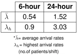
ThinkPad E550 with Intel(R) Core(TM) i5-5200 CPU @ 2.20GHz processor (8GB RAM). We use the parameters that are inspired by the cases in Jeroen Bosch Ziekenhuis (JBZ), Den Bosch in 2017 and RSUP Sardjito (Hospital), Yogyakarta, Indonesia in May-August 2019. For both hospitals, we look at the data where each OR day is divided into 4 shifts, each of 6-hour length. We calculate the arrival rate of each patient type per shift. The arrival rates of the 6-hour and 24-hour patients at JBZ in 2017 are given in the following table.

6-hour 24-hour

¯

λ 0.54 1.52 λh 0.9 3.03 *¯_{λ= average arrival rates}

λh= highest arrival rates

[image:24.595.246.381.538.633.2]

(no.of patients/shift)

Table 3.1: Arrival rates of the 6-hour and 24-hour patients in the JBZ dataset

(25)

No Arr. rate (patients/shift)

1 _{24-hour patients :}6-hour patients : 0.54 1.2

2 6-hour patients : 0.54

24-hour patients : 1.52 3 6-hour patients : 0.9

24-hour patients : 3.03

*Arr. rate = arrival rate of each patient type per shift (no.of patients/shift); s = the maximum number of surgeries that can be performed in the dedicated capacity.

Table 3.2: The various arrival rates for case study on queueing models based on JBZ dataset

In the next parts, we conduct numerical experiments for the cases above using M/M/1/4s andM/M/1with priority rule queueing models.

Whereas in RSUP Sardjito, only arrivals of the 24-hour patients take place. The arrival rate is 0.817 patients per shift in average, where 1.82 patients per shift is the highest arrival rate. For this case, we only conduct a case study using M/M/1/4s queueing model as there is only one type patient in the system.

3.3.1 Case study on

M/M/

1 /

4 s

queueing model

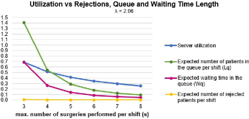
InM/M/1/4squeueing model, the dedicated OR has a capacity ofµ=s surgeries per shift. The maximum number of patients in the system, 4s, is obtained by con-sidering that the 24-hour patients can afford to wait up to 4 shifts upon their arrivals. The case study is conducted for the arrival rates given in Table5.4. For each case, we look at the server utilization compared to the expected number of rejected pa-tients, queue length and waiting time in the queue.

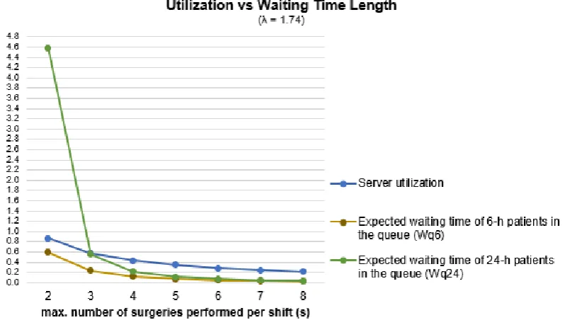
For the first case, where λ6 = 0.54 and λ24 = 1.2, the sensitivity analysis is per-formed by takings = 2tos = 8.The chart in Figure3.1shows the server utilization along with the expected number of rejected patients, queue length and waiting time length in each shift. We can observe that the higher server utilization yields in the larger queue length, which implies a longer waiting time and more rejected patients. For example, take the case where s = 2.The server utilization is around 0.8, while

the expected queue length is around 2.3 patients per shift (≈8 patients a day) and

the expected waiting time is 1.4 shifts where in average 0.1 patients are rejected per shift. The maximum capacity that we test is not larger thans = 8, because we can

see that froms = 3tos= 8 no patients are rejected (all arrivals can be admitted).

(26)

[image:26.595.97.530.82.319.2]

Figure 3.1:Sensitivity analysis forλ6 = 0.54andλ24 = 1.2

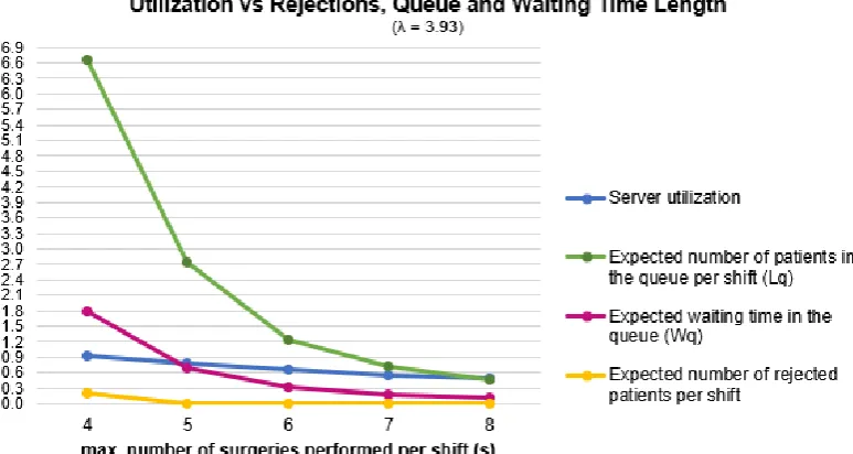
3.3 respectively illustrate the server utilization along with the expected number of rejected patients, queue length, and waiting time length in each shift for different capacitys. Similar with the first case, in these two cases, the higher utilization yields in larger expected queue length and longer expected waiting time. The highest

Figure 3.2:Sensitivity analysis forλ6 = 0.54andλ24= 1.52

server utilization of arund 0.9 is reached fors = 4. However, for this case, the

ex-pected number of patients waiting in a shift is 6.6 and in average we reject around 0.3 patient in a shift (≈2 patients in a day). The expected queue length drops to 2.7

[image:26.595.93.529.430.639.2]

(27)

[image:27.595.117.504.90.296.2]

Figure 3.3: Sensitivity analysis forλ6 = 0.9andλ24 = 3.03

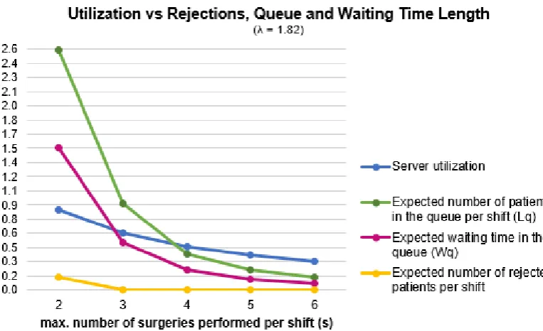
Next, the results of the case study for the dataset from RSUP Sardjito are pre-sented in Figures3.4and3.5forλ= 0.817andλ= 1.82, respectively. Same as the

Figure 3.4: Sensitivity analysis forλ24 = 0.817

previous results on JBZ dataset, the higher utilization results in larger mean queue length and longer mean waiting time.

[image:27.595.118.506.416.617.2]

(28)

[image:28.595.117.499.85.318.2]

Figure 3.5: Sensitivity analysis forλ24= 1.82

3.3.2 Case study on

M/M/

1 with priority rule queueing model

InM/M/1with priority queueing model, the queue has one dedicated OR (server)

with service rate of µ patients per shift. By looking at Assumption 3.1.2, we have µ = s patients per shift. The two type patients are treated using non-preemptive priority rule, where the 6-hour patients have priority over the 24-hour patients.

First, we look at the server utilization and expected waiting time for 6-hour and 24-hour patients, where λ = 1.74 and s = 2 to s = 8 given in Figure 3.6. We also

observe the server utilization and expected queue length for 6-hour and 24-hour patients for this case in Figure3.7. The sensitivity analysis results using other pa-rameters in Table5.4for this model are given in the Appendix A.

Recall that in the data from RSUP Sardjito there is no 6-hour patient arrivals, i.e., λ6 = 0.Hence, theM/M/1with priority queueing model is not suitable for this data as we only have one patient type: 24-hour patients.

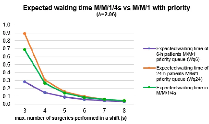
Last, we compare the mean waiting time in M/M/1/4s andM/M/1priority

queue-ing models for the parameters in Table5.4. The comparison of these models when λ6 = 0.54,λ24= 1.2is given in the following chart. We can see from the chart in Fig-ure3.8 that fors = 2 in the M/M/1priority queueing model the waiting time of the

(29)

[image:29.595.113.512.89.315.2]

Figure 3.6: Sensitivity analysis on the mean waiting time forλ6 = 0.54 ; λ24 = 1.2 using

priority rule

Figure 3.7: Sensitivity analysis on the mean queue lengthλ= 1.74using priority rule

waiting times of both patients drop when the hospital has a capacity of at leasts= 3.

Fors = 4, the mean waiting times of both patient types in the two queueing models

are close, where the gaps are getting smaller assgets larger.

[image:29.595.115.514.372.612.2]

(30)

[image:30.595.136.482.345.551.2]

Figure 3.8: Expected waiting time forλ6 = 0.54andλ24= 1.2inM/M/1/4sandM/M/1priority

queueing models

Figure 3.9: Expected waiting time forλ6 = 0.54andλ24= 1.52inM/M/1/4sandM/M/1

priority queueing models

From the results in the two queueing models in the three last figures, we can con-clude that high utilization results in large queue length and waiting time (other figures are attached in AppendixA).

(31)

pri-Figure 3.10: Expected waiting time forλ6 = 0.9andλ24= 3.03inM/M/1/4sandM/M/1

priority queueing models

(32)

Chapter 4

Model for scheduling urgent

surgeries independent of elective

surgeries

This chapter formulates four models to schedule urgent surgeries independent of the elective patients based on Markov decision processes (MDP) which employs the infinite planning horizon for the hospital that uses dedicated operating rooms to perform urgent surgeries.

This chapter is structured as follows: Section 4.1 describes what Markov decision processes is, Section4.2gives the assumptions that are used to formulate the mod-els, Section 4.3 describes the MDP to decide the number of urgent surgeries per-formed in each part of the day along with the MDP that allows deferring the patients to other resources in Subsection 4.3.1, Section 4.4 explains the MDP to assign a number of urgent surgeries to the appropriate time.

4.1 Markov decision processes (MDP)

(33)

im-portant than those incurred in the future. More about MDP can be found in [20].

In the next sections, as we build the model using a Markov decision processes (MDP), the following elements are needed [20]:

1. Decision epochs. 2. States.

3. Actions.

4. Transition probabilities. 5. Direct costs.

In formulating the models, the assumptions used are explained in the next section.

4.2 Assumptions

This section explains the assumptions made to build the models. Recall the urgent patients categories in Table 1.1. Assumption 4.2.1 gives the policy to handle the 30-minute surgeries.

Assumption 4.2.1. 30-minute surgeries are performed within the shift where they arrive.

Assumption4.2.1implies that the 30-minute surgeries are scheduled and hence will not be considered in the models. Assumption 4.2.2 gives the distribution of urgent patient arrivals.

Assumption 4.2.2. Each type of urgent patient arrives at a shift according to a Poisson process. The arrival process within a shift is independent of the arrival processes in other shifts.

A Poisson process is a counting process. The definition of a counting process is shown in Definition4.2.3. The definition of a Poisson process is shown in Definition

4.2.4.

Definition 4.2.3. [21] A stochastic process {N(t), t ≥ 0} is said to be a counting process ifN(t)represents the total number of events that occur by timet.

Definition 4.2.4. [21] The counting process {N(t), t ≥ 0} is said to be a Poisson process having rateλ >0if

1. N(0) = 0

(34)

Assigning a number of urgent patients in each shift (Model 1) 24

3. The number of events in any interval of length t is Poisson distributed with meanλ t. That is, for alls, t≥0

P(N(t+s)−N(s) =n) = eλ.t (λ.t)n

n! , n= 0,1,2, . . . . (4.1)

In further part of this report, the Poisson probability above is denoted by

P oi(n, λ.t).

The daily OR time is divided into four shifts: morning, afternoon, evening and night. Assumption4.2.5is needed to make the decision for each urgent surgery type. Assumption 4.2.5. The 6-hour patients should be scheduled one shift ahead of the arriving shift and the 24-hour patients can wait up to four shifts upon the arriving shift.

The models are constructed for hospitals that dedicate some capacity for urgent pa-tients. Letsn denote the maximum number of urgent patients that can be performed

in shift n using the dedicated capacity. Assumption4.2.6 gives the maximum num-ber of surgeries that can be performed in each shift that we take into account in the models.

Assumption 4.2.6. The maximum number of urgent surgeries that can be per-formed within each shift is identical, regardless of the type of surgeries. Hence, we havesn=sfor alln ∈N.

In Sections4.3and4.4we describe the MDP model to schedule the urgent patients by observing the arrivals until the end of each shift where an action should be taken.

4.3 Assigning a number of urgent patients in each

shift (Model 1)

In this section we describe the MDP model to schedule urgent patients, where in each shift we determine the number urgent surgeries of each type that are assigned in the next shift.

Decision epochs

(35)

Figure 4.1:Decision epoch The notation for the decision epoch is given by:

N={1,2,3, . . .}, n∈_N.

State space

The state at the end of shift n ∈ _N is the number of urgent cases that can wait for

a maximum of t more shifts upon its arrival. By employing Assumption 4.2.5, the definition below is given to model the state space.

Definition 4.3.1. Let a stochastic process{Un, n= 1,2,3, . . .}, where

Un= (U1,n, U2,n, U3,n, U4,n),∀n∈N

andUt,nrecords the number of urgent patients that are allowed to wait fort shifts in

the system at the end of shiftn,∀n ∈_N, t= 1,2,3,4.

Letudenote the realization of the random variableU in Definition4.3.1. Hence, the state at the end of shiftn is denoted by:

un = (u1,n;u2,n; u3,n; u4,n).

All possible states at decision epochn build the entire state spaceS, which is given by:

S={Sn}n∈N,

where

Sn ={un = (u1,n; u2,n; u3,n; u4,n)|u1,n, u2,n, u3,n, u4,n = 0,1,2, . . . <∞} ∀n∈N.

(4.2)

Boundary of the states

By looking at the definition of the states above and Assumption4.2.6, the total num-ber of surgeries in the system within each shift should not exceed 4s, which is

for-mulated in the following equation: 4 X

t=1

(36)

Decisions

The decision in each shift is to determine the number of urgent surgeries that are performed in the next shift. Other than the maximum waiting time of urgent surgeries that is given by Assumption4.2.5, the decisions should satisfy the conditions below: 1. If some surgeries are not yet assigned, then they can wait for one shift less. For example, if in shift n ∈ _N the state is given by un = (0,1,1,1) and no surgeries are assigned to the next shift, then in the next shift the state is

un+1= (1,1,1,0).

2. The sum of the surgeries that are assigned in each shift should not exceed the dedicated capacity.

The notation for the action is as follows:

Au,n ={an = (a1,n, a2,n, a3,n, a4,n) = (doat,nsurgery out ofut,n, t= 1,2,3,4),

∀n ∈_N|at,n≤ut,n,

4 X

t=1

at,n≤s, t = 1,2,3,4, ∀n∈N},

A= [

u∈S,n∈_N

Au,n.

Transition probabilities

In formulating the transition probabilities, we take patient arrivals into account. Let random variableRp,n denote the number of typeppatients that arrive to the system

at shiftn, wherep = 6 and p = 24represent the 6-hour and 24-hour surgeries,

re-spectively. Using Assumption 4.2.2, Rp,n follows a Poisson process with an arrival

rate ofλp, wherep= 6,24,for alln ∈N.

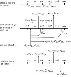
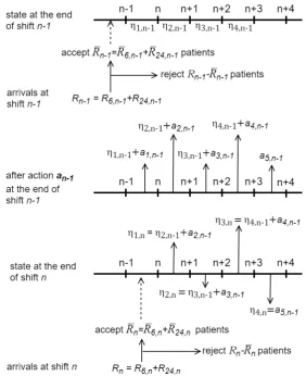
The evolution of the states given by the diagram in Figure 4.2 is used to construct the transition probability. Also, based on Assumption4.2.6, the following assumption describes the policy to admit the arriving patients.

Assumption 4.3.2. First, the maximum number of 6-hour patients are admitted to fill the slot s. Next, the 24-hour patients are admitted such that the total number of patients within a shift does not exceed4s. In case the system is full, i.e., there are

4s patients in the system, we reject all arrivals from entering the system.

Let _R¯_p,n _{denote the number of type} _p _{patient arrivals that are admitted at shift} _n,

where p = 6,24 denoting 6-hour and 24-hour patients, respectively. Next, from

(37)

[image:37.595.160.447.89.400.2]

Figure 4.2: State evolution from shiftn−1to shiftn

we admit _R¯₂₄_,n _{24-hour arrivals, where}_R¯₂₄_,n _{= min}_{_R₂₄_,n_,₄_s₋₍_u₁_,n ₊_u₂_,n ₊_u₃_,n₎_}_.

Hence,u4,n = min{R24,n,4s−(u1,n+u2,n+u3,n)}.

To formulate the transition probability further, the definition of the exponential dis-tribution is given in Definition4.3.3. The definition of the Erlang distribution is shown in Definition4.3.4.

Definition 4.3.3. [21] A continuous random variableX is said to have an exponen-tial distribution with parameterλ,λ > 0if its probability density function is given by

f(x) =λ e−λ x, x≥0 (4.4)

or, equivalently, if its cumulative distribution function is given by

F(x) = Z x

−∞

f(y)dy= 1−e−λ x, x≥0. (4.5) Definition 4.3.4. A random variableXhas an Erlang-k(k = 1,2, . . .) distribution with meank/λ, ifX is the sum of k independent random variablesX1, . . . , Xk having an

(38)

by

fErl(x;k, λ) =λ

(λ x)k−1 (k−1)!e

−λ x_{, x}_≥₀_. _(4.6)

The cumulative distribution function is given by

FErl(x;k, λ) = 1− k−1 X

j=0 (λ x)j

j! e

−λ x_{, x}_≥₀_. _(4.7)

The parameterλis called the scale parameter,k is the shape parameter.

For the transition probability, we use the notation below:

P(un|un−1,an−1) =P(U1,n =u1,n, U2,n =u2,n, U3,n =u3,n, U4,n =u4,n|

U1,n−1 =u1,n−1, U2,n−1 =u2,n−1, U3,n−1 =u3,n−1, U4,n−1 =u4,n−1,

an−1 = (a1,n−1, a2,n−1, a3,n−1, a4,n−1))

=_P(u1,n = min{u2,n−1−a2,n−1+R6,n, s}, u2,n =u3,n−1−a3,n−1, u3,n =u4,n−1−a4,n−1, u4,n = min{R24,n,4s−(u1,n+u2,n+u3,n)}|

R6,n ≥0, R24,n ≥0). (4.8)

Employing Assumption4.3.2and state evolution in Figure4.2, we build the transition probabilities based on the patient arrivals.

Ifu2,n−1−a2,n−1+R6,n < s, then at the end of shiftnthe first element of the state is

u1,n =u2,n−1−a2,n−1+R6,n < s. After that, ifu1,n+u2,n+u3,n+R24,n <4sthenu4,n =

R24,n. Hence, the state at the end of shiftnisu1,n < s, u1,n+u2,n+u3,n +u4,n <4s,

which transition probability is as follows:

an−1 = (a1,n−1, a2,n−1, a3,n−1, a4,n−1))

=_P(u1,n =u2,n−1−a2,n−1+R6,n, u2,n =u3,n−1−a3,n−1, u3,n =u4,n−1−a4,n−1, u4,n =R24,n)

=_P(R6,n =u1,n−u2,n−1+a2,n−1, R24,n =u4,n)

=_P(R6,n =u1,n−u2,n−1+a2,n−1) × P(R24,n =u4,n)

=e−λ6_e−λ24 λ

u1,n−u2,n−1+a2,n−1 6

(u1,n−u2,n−1+a2,n−1)! .λ

u4,n 24 u4,n!

,

=P oi(u1,n−u2,n−1+a2,n−1, λ6). P oi(u4,n, λ24) (4.9) u1,n < s; u1,n+u2,n+u3,n+u4,n <4s.

(39)

end of shift n, the state is given by u1,n < s, u1,n +u2,n +u3,n +u4,n = 4s, which is

equivalent tou1,n < s, u4,n = 4s−(u1,n+u2,n+u3,n). Thus, for this case we have the

following transition probability:

an−1 = (a1,n−1, a2,n−1, a3,n−1, a4,n−1))

=_P(u1,n =u2,n−1−a2,n−1+R6,n, u2,n =u3,n−1−a3,n−1, u3,n =u4,n−1−a4,n−1, u4,n = 4s−(u1,n+u2,n+u3,n))

=_P(R6,n =u1,n−u2,n−1+a2,n−1, u2,n =u3,n−1−a3,n−1,

u3,n =u4,n−1−a4,n−1, R24,n ≥4s−(u1,n+u2,n+u3,n))

=_P(R6,n =u1,n−u2,n−1+a2,n−1,

R24,n ≥4s−(u1,n+u2,n+u3,n))

=_P(R6,n =u1,n−u2,n−1+a2,n−1)

× _P(R24,n ≥4s−(u1,n+u2,n+u3,n))

=e−λ6 λ

u1,n−u2,n−1+a2,n−1 6

(u1,n−u2,n−1 +a2,n−1)! .

∞ X

r24=4s−(u1,n+u2,n+u3,n)

e−λ24λ

r24 24 r24!

=e−λ6 λ

u1,n−u2,n−1+a2,n−1 6

(u1,n−u2,n−1 +a2,n−1)! .



1−

4s−(u1,n+u2,n+u3,n)−1 X

r24=0

e−λ24λ

r24 24 r24!





=P oi(u1,n−u2,n−1+a2,n−1, λ6). FErl(4s−(u1,n+u2,n+u3,n), λ24), (4.10) u1,n < s; u1,n+u2,n+u3,n+u4,n = 4s,

where FErl(k, λ) is the cumulative distribution function of the Erlang-k distribution

with scale parameterλ.

If u2,n−1 −a2,n−1 +R6,n ≥ s, then at the end of shift n the first element of the state

is u1,n = s. Next, if u1,n +u2,n +u3,n +R24,n < 4s, then at the end of shift n the

last element of the state is u4,n = R24,n. Hence, the state at the end of shift n is

u1,n =s, u1,n+u2,n+u3,n+u4,n <4s and the transition probability is given by:

(40)

=_P(u1,n =s, u2,n =u3,n−1−a3,n−1, u3,n =u4,n−1−a4,n−1, u4,n =R24,n)

=_P(s ≤u2,n−1−a2,n−1+R6,n, u2,n =u3,n−1 −a3,n−1, u3,n =u4,n−1−a4,n−1, u4,n =R24,n)

=_P(R6,n ≥s−u2,n−1+a2,n−1, R24,n =u4,n)

=_P(R6,n ≥s−u2,n−1+a2,n−1) × P(R24,n =u4,n)

=e−λ24

∞ X

r6=s−u2,n−1+a2,n−1

e−λ6λ

r6 6 r6!

.λ

u4,n 24 u4,n!

=e−λ24 λ

u4,n 24 u4,n!

1−

s−u2,n−1+a2,n−1−1 X

r6=0

e−λ6 λ

r6 6 r6!

!

=P oi(u4,n, λ24). FErl(s−u2,n−1+a2,n−1, λ6) (4.11) u1,n =s ; u1,n+u2,n+u3,n+u4,n <4s.

is u1,n = s. Next, if u1,n +u2,n +u3,n +R24,n ≥ 4s, then at the end of shift n the

state is given by u1,n = s, u1,n +u2,n +u3,n +u4,n = 4s, which is equivalent to

u1,n =s, u4,n = 3s−(u2,n+u3,n)and the transition probability is given by:

an−1 = (a1,n−1, a2,n−1, a3,n−1, a4,n−1)) =_P(u1,n =s, u2,n =u3,n−1−a3,n−1,

u3,n =u4,n−1−a4,n−1, u4,n = 3s−(u2,n+u3,n))

=_P(s≤u2,n−1−a2,n−1+R6,n, u2,n=u3,n−1−a3,n−1, u3,n =u4,n−1−a4,n−1, 3s−(u2,n+u3,n)≤R24,n)

=_P(R6,n ≥s−u2,n−1+a2,n−1, R24,n ≥3s−u2,n−u3,n)

=_P(R6,n ≥s−u2,n−1+a2,n−1) × P(R24,n ≥3s−u2,n−u3,n)

=e−λ6_e−λ24

∞ X

r6=s−u2,n−1+a2,n−1 λr6

6 r6!

.

∞ X

r24=3s−u2,n−u3,n

λr24 24 r24!

= 1−

s−u2,n−1+a2,n−1−1 X

r6=0

e−λ6 λ

r6 6 r6!

!

. 1−

3s−u2,n−u3,n−1 X

r24=0

e−λ24 λ

r24 24 r24!

!

(41)

Direct cost

The first cost incurred because of the rejections of the 6-hour patient arrivals from entering the system. From Assumption4.3.2we know that ifu1,n ≤s, all 6-hour

pa-tients can be treated in the dedicated capacity. Ifu2,n−1 −a2,n−1+R6,n > swe need

to rejectu2,n−1 −a2,n−1+R6,n−spatients. Note that at shiftn,u1,n depends on the

state and action at shiftn−1asu1,n= min{u2,n−1−a2,n−1+R6,n, s}, whereR6,n is the

6-hour patient arrivals at shiftn. Denoting the number of 6-hour surgeries being re-jected at shiftn byNe,n, the formula to compute its expectation, E[Ne,n|un−1, an−1],

is:

E[Ne,n|un−1, an−1] =E[u2,n−1−a2,n−1+R6,n−s]+

= ∞ X

r6=0

(u2,n−1−a2,n−1+r6−s)+P(R6,n =r6)

=

∞ X

r6=s−u2,n−1+a2,n−1+1

(u2,n−1−a2,n−1+r6 −s)P(R6,n =r6)

=

∞ X

r6=s−u2,n−1+a2,n−1+1

(u2,n−1−a2,n−1−s)P(R6,n =r6)

+

∞ X

r6=s−u2,n−1+a2,n−1+1

r6 P(R6,n =r6)

= (u2,n−1−a2,n−1−s) 1−

s−u2,n−1+a2,n−1 X

r6=0

P(R6,n =r6) !

+ ∞ X

r6=0

r6 P(R6,n =r6)−

s−u2,n−1+a2,n−1 X

r6=0

r6 P(R6,n =r6)

= (u2,n−1−a2,n−1−s) 1−

s−u2,n−1+a2,n−1 X

r6=0

e−λ6 λ

r6 6 r6!

!

+_E[R6,n]

−

s−u2,n−1+a2,n−1 X

r6=0

r6 e−λ6 λr6

6 r6!

= (u2,n−1−a2,n−1−s) 1−

s−u2,n−1+a2,n−1 X

r6=0

e−λ6 λ

r6 6 r6!

! +λ6

−

s−u2,n−1+a2,n−1 X

r6=0

r6 e−λ6 λr6

6 r6!

.

(4.13) LetN =u2,n−1−a2,n−1−s. We have:

s−u2,n−1+a2,n−1 X

r6=0

r6 e−λ6 λr6

6 r6!

=

N

X

n=0

n e−λ6 λ

n

6

(42)

and is elaborated as follows:

N

X

n=0

n e−λ6 λ

n

6 n! =

N

X

n=1

n e−λ6 λ

n 6 n! = N X n=1

e−λ6 λ

n

6 (n−1)!

=λ6

N

X

n=1

e−λ6 λ

n−1 6 (n−1)!

=λ6

N

X

n=1

e−λ6 λ

n−1 6 (n−1)!

=λ6

N−1 X

m=0

e−λ6 λ

m

6 m!

=λ6(1−FErl(N, λ6)). (4.15) Substituting Equation (4.15) to Equation (4.13), we obtain:

E[Ne,n|un−1, an−1] = (u2,n−1−a2,n−1−s) 1−

s−u2,n−1+a2,n−1 X

r6=0

e−λ6 λ

r6 6 r6!

! +λ6

−λ6(1−FErl(s−u2,n−1+a2,n−1, λ6)) = (u2,n−1−a2,n−1−s)FErl(s−u2,n−1+a2,n−1 + 1, λ6)

+λ6FErl(s−u2,n−1+a2,n−1, λ6),∀n∈N. (4.16) Another cost is incurred from rejecting the 24-hour surgeries because of the bound-ary of the state. Denoting the number of 24-hour surgeries being rejected at shiftn by_Nˆ

e,n, it is formulated as follows:

ˆ

Ne,n = (u1,n+u2,n+u3,n+R24,n−4s)+,∀n ∈N. (4.17)

Recall that the state at shiftn depends on the state un−1 and action an−1.Hence,

E[ ˆNe,n|un−1, an−1]is formulated as follows.

E[ ˆNe,n|un−1, an−1] =E[(u1,n+u2,n+u3,n+R24,n−4s)+|un−1, an−1]

=_E[(u2,n−1−a2,n−1+R6,n+u2,n+u3,n+R24,n−4s)+]

= ∞ X

r6=0

∞ X

r24=0

(u2,n−1−a2,n−1+r6+u2,n+u3,n+r24−4s)+

(43)

=

s−(u2,n−1

−a2,n−1)−1 X

r6=0

∞ X

r24=4s−(u2,n−1

−a2,n−1+r6+u2,n +u3,n)+1

(u2,n−1 −a2,n−1+r6+u2,n+u3,n

+r24−4s)P(R6,n =r6)P(R24,n =r24)

+

∞ X

r6=s−(u2,n−1−a2,n−1)

∞ X

r24=3s−(u2,n +u3,n)+1

(s+u2,n+u3,n

+r24−4s)P(R6,n =r6)P(R24,n =r24)

= (u2,n−1−a2,n−1+u2,n+u3,n−4s)

s−(u2,n−1

−a2,n−1)−1 X

r6=0

P(R6,n =r6)

∞ X

r24=4s−(u2,n−1

−a2,n−1+r6+u2,n +u3,n)+1

P(R24,n=r24)

+

s−(u2,n−1

−a2,n−1)−1 X

r6=0

∞ X

r24=4s−(u2,n−1

−a2,n−1+r6+u2,n +u3,n)+1

r6P(R6,n =r6)P(R24,n =r24)

+

s−(u2,n−1

−a2,n−1)−1 X

r6=0

∞ X

r24=4s−(u2,n−1

−a2,n−1+r6+u2,n +u3,n)+1

r24P(R6,n =r6)P(R24,n =r24)

+ (s+u2,n+u3,n−4s)

∞ X

r6=s−(u2,n−1−a2,n−1)

∞ X

r24=3s−(u2,n +u3,n)+1

P(R6,n =r6)P(R24,n =r24)

+

∞ X

r6=s−(u2,n−1−a2,n−1)

P(R6,n =r6)

∞ X

r24=3s−(u2,n +u3,n)+1

r24P(R24,n =r24)

= (u2,n−1−a2,n−1+u2,n+u3,n−4s)

s−(u2,n−1

−a2,n−1)−1 X

r6=0

P(R6,n =r6)

      1−

4s−(u2,n−1

−a2,n−1+r6+u2,n +u3,n)

X

r24=0

(44)

+

s−(u2,n−1

−a2,n−1)−1 X

r6=0

r6P(R6,n =r6)       1−

4s−(u2,n−1

−a2,n−1+r6+u2,n +u3,n)

X

r24=0

P(R24,n =r24)       +

s−(u2,n−1

−a2,n−1)−1 X

r6=0

P(R6,n =r6)       ∞ X

r24=0

r24P(R24,n =r24)−

4s−(u2,n−1

−a2,n−1+r6+u2,n +u3,n)+1

X

r24=0

r24P(R24,n =r24)      

+ (u2,n+u3,n−3s)



  

1−

s−(u2,n−1

−a2,n−1)−1 X

r6=0

P(R6,n =r6)         1−

3s−(u2,n +u3,n)

X

r24=0

P(R24,n =r24     +     1−

s−(u2,n−1

−a2,n−1)−1 X

r6=0

P(R6,n =r6)         ∞ X

r24=0

r24P(R24,n =r24)−

3s−(u2,n +u3,n)

X

r24=0

r24P(R24,n =r24) 

  

= (u2,n−1−a2,n−1+u2,n+u3,n−4s)

s−(u2,n−1

−a2,n−1)−1 X

r6=0

P(R6,n =r6)

      1−

4s−(u2,n−1

−a2,n−1+r6+u2,n +u3,n)

X

r24=0

P(R24,n =r24)       +

s−(u2,n−1

−a2,n−1)−1 X

r6=0

r6P(R6,n =r6)       1−

4s−(u2,n−1

−a2,n−1+r6+u2,n +u3,n)

X

r24=0

P(R24,n =r24)       +

s−(u2,n−1

−a2,n−1)−1 X

r6=0

P(R6,n =r6)      

λ24−

4s−(u2,n−1

−a2,n−1+r6+u2,n +u3,n)+1

X

r24=0

r24P(R24,n =r24)      

+ (u2,n+u3,n−3s)



  

1−

s−(u2,n−1

−a2,n−1)−1 X

r6=0

P(R6,n =r6)         1−

3s−(u2,n +u3,n)

X

r24=0

P(R24,n =r24     +     1−

s−(u2,n−1

−a2,n−1)−1 X

r6=0

P(R6,n =r6)        

λ24−

3s−(u2,n +u3,n)

X

r24=0

r24P(R24,n =r24) 

(45)

= (u2,n−1−a2,n−1+u2,n+u3,n−4s)

s−(u2,n−1

−a2,n−1)−1 X

r6=0

P oi(r6, λ6)

FErl(4s−(u2,n−1−a2,n−1+r6+u2,n+u3,n) + 1, λ24)

+

s−(u2,n−1

−a2,n−1)−1 X

r6=0

r6P oi(r6, λ6)FErl(4s−(u2,n−1−a2,n−1+r6+u2,n+u3,n) + 1, λ24)

+

s−(u2,n−1

−a2,n−1)−1 X

r6=0

P oi(r6, λ6)(λ24−λ24(1−FErl(4s−(u2,n−1−a2,n−1+r6+u2,n+u3,n) + 1,

λ24))) + (u2,n+u3,n−3s)FErl(s−(u2,n−1−a2,n−1), λ6)FErl(3s−(u2,n+u3,n) + 1,

λ24) +FErl(s−(u2,n−1−a2,n−1), λ6)(λ24−λ24(1−FErl(3s−(u2,n+u3,n), λ24)))

= (u2,n−1−a2,n−1+u2,n+u3,n−4s)

s−(u2,n−1

−a2,n−1)−1 X

r6=0

P oi(r6, λ6)

FErl(4s−(u2,n−1−a2,n−1+r6+u2,n+u3,n) + 1, λ24)

+

s−(u2,n−1

−a2,n−1)−1 X

r6=0

r6P oi(r6, λ6)FErl(4s−(u2,n−1−a2,n−1+r6+u2,n+u3,n) + 1, λ24)

+

s−(u2,n−1

−a2,n−1)−1 X

r6=0

P oi(r6, λ6)λ24FErl(4s−(u2,n−1−a2,n−1+r6+u2,n+u3,n) + 1, λ24)

+ (u2,n+u3,n−3s)FErl(s−(u2,n−1−a2,n−1), λ6)FErl(3s−(u2,n+u3,n) + 1, λ24) +FErl(s−(u2,n−1−a2,n−1), λ6)λ24FErl(3s−(u2,n+u3,n), λ24).

(4.18) Given the stateunand actionanthe number of unused capacityNu,ncan be

formu-lated as follows:

Nu,n= s−

4 X t=1 at,n !+ 1 4 X t=1

ut,n >0

!

,∀n ∈_N. (4.19)

Let ce, cˆe, and cu denote the cost of one rejected 6-hour patient, one rejected

24-hour patient, and one unused dedicated capacity, respectively. Henceforth, by using Equations (4.16), (4.19) and (4.18) we obtain the expected total costs in shiftnis:

(46)

Optimality equation

We consider the costs incurred today to be more important than those that are in-curred tomorrow. Therefore we use discount factor α, α ∈ [0,1) to recalculate the

future costs to the cost level today. The goal is to minimize the rejected patients and utilize the dedicated capacity optimally. This can be done by minimizing the expected discounted cost over an infinite horizon, because the costs are incurred from the unused dedicated capacity and rejecting patients from entering the sys-tem. Therefore, the optimality equation is as follows:

V(u)= min

a∈A

(

c(u, a0) +α

X

u0

P(u0|u, a)V(u0) )

. (4.21)

The optimal policyA∗ consists of the values ofathat solve the optimality equation in each state. We use the policy iteration algorithm to find the optimal policyA∗. Algorithm 1Policy iteration algorithm

1: i←0

2: A0 ←A¯ .Choose an arbitrary policyA¯∈A 3: whileAi+16=Ai do

4: foreach stateun∈S do

5: Policy Evaluation :Vi(un) =c(un, Ai) +αP_u0

nP(u

0

n|un,Ai)V(u0n) 6: Policy improvement:

7: Ai+1 ∈arg min

A

{c(un, A) +αP_u0

nP(u

0

n|un, A)Vi(u0n)}

8: end for 9: i←i+ 1

10: end while

11: returnA∗ =Ai .The optimal policyA∗

4.3.1 Enable deferring the 24-hour patients to another resource

(Model 1b)

(47)

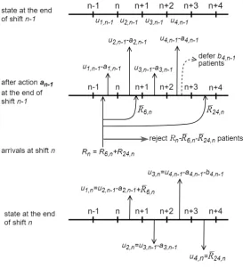
In this part the state of the system is described by Equation (4.2). The decisions now include deferring the 24-hour patients to another resource, denoted by b4,n.

Note that the total 24-hour surgeries that are performed and deferred to other re-source should not exceed the existing 24-hour patients in the system, formulated by a4,n+b4,n ≤u4,n.With this modification, the decisions are denoted as follows:

Au,n ={an = (a1,n, a2,n, a3,n, a4,n, b4,n) = (doat,n surgery out ofut,n, t= 1,2,3,

deferring b4,n 24-hour patients)|at,n≤ut,n, t= 1,2,3 ;a4,n+b4,n ≤u4,n,

4 X

t=1

at,n ≤s, ∀n∈N},

A= [

u∈S,n∈N

Au,n.

[image:47.595.170.444.336.638.2]

The evolution of the states is given in the diagram in Figure4.3.

Figure 4.3: State evolution from the beginning of shift n −1 to the end of shift n while allowing 24-hour patients to be deferred

(48)

the transition probability. The following notation is used :

an−1 = (a1,n−1, a2,n−1, a3,n−1, a4,n−1, b4,n−1))

=_P(u1,n = min{u2,n−1−a2,n−1+R6,n, s}, u2,n =u3,n−1−a3,n−1, u3,n =u4,n−1−a4,n−1−b4,n−1, u4,n = min{R24,n,4s−(u1,n+

u2,n+u3,n)}|R6,n ≥0, R24,n ≥0). (4.22)

Based on the arrivals, if u2,n−1 −a2,n−1 +R6,n < s, then at the end of shift n the

first element of the state is u1,n = u2,n−1 −a2,n−1 +R6,n < s. After that, if u1,n +

u2,n +u3,n+R24,n < 4s then u4,n = R24,n. Hence, the state at the end of shift n is

u1,n < s, u1,n+u2,n+u3,n+u4,n <4s, which transition probability is as follows:

an−1 = (a1,n−1, a2,n−1, a3,n−1, a4,n−1, b4,n−1))

=_P(u1,n =u2,n−1−a2,n−1+R6,n, u2,n =u3,n−1−a3,n−1, u3,n =u4,n−1−a4,n−1−b4,n−1, u4,n =R24,n)

=_P(R6,n =u1,n−u2,n−1+a2,n−1, R24,n =u4,n)

=_P(R6,n =u1,n−u2,n−1+a2,n−1) × P(R24,n =u4,n)

=e−λ6_e−λ24 λ

u1,n−u2,n−1+a2,n−1 6

(u1,n−u2,n−1+a2,n−1)! .λ

u4,n 24 u4,n!

,

=P oi(u1,n−u2,n−1+a2,n−1, λ6). P oi(u4,n, λ24) (4.23) u1,n < s; u1,n+u2,n+u3,n+u4,n <4s.

u1,n = u2,n−1 −a2,n−1+R6,n < s. Next, if u1,n+u2,n +u3,n +R24,n ≥ 4s, then at the

end of shift n, the state is given by u1,n < s, u1,n +u2,n +u3,n +u4,n = 4s, which is

equivalent tou1,n < s, u4,n = 4s−(u1,n+u2,n+u3,n). Thus, for this case we have the

following transition probability:

an−1 = (a1,n−1, a2,n−1, a3,n−1, a4,n−1, b4,n−1))

=_P(u1,n =u2,n−1−a2,n−1+R6,n, u2,n =u3,n−1−a3,n−1,

(49)

=_P(R6,n =u1,n−u2,n−1+a2,n−1, u2,n =u3,n−1−a3,n−1,

u3,n =u4,n−1−a4,n−1−b4,n−1, R24,n ≥4s−(u1,n+u2,n+u3,n))

=_P(R6,n =u1,n−u2,n−1+a2,n−1,

R24,n ≥4s−(u1,n+u2,n+u3,n))

=_P(R6,n =u1,n−u2,n−1+a2,n−1)

× _P(R24,n ≥4s−(u1,n+u2,n+u3,n))

=e−λ6 λ

u1,n−u2,n−1+a2,n−1 6

(u1,n−u2,n−1+a2,n−1)! .

∞ X

r24=4s−(u1,n+u2,n+u3,n)

e−λ24λ

r24 24 r24!

=e−λ6 λ

u1,n−u2,n−1+a2,n−1 6

(u1,n−u2,n−1+a2,n−1)! .



1−

4s−(u1,n+u2,n+u3,n)−1 X

r24=0

e−λ24λ

r24 24 r24!





=P oi(u1,n−u2,n−1+a2,n−1, λ6). FErl(4s−(u1,n+u2,n+u3,n), λ24), (4.24) u1,n < s; u1,n+u2,n+u3,n+u4,n = 4s,

where FErl(k, λ) is the cumulative distribution function of the Erlang-k distribution

with scale parameter ofλ.

is u1,n = s. Next, if u1,n +u2,n +u3,n +R24,n < 4s, then at the end of shift n the

last element of the state is u4,n = R24,n. Hence, the state at the end of shift n is

u1,n =s, u1,n+u2,n+u3,n+u4,n <4s and the transition probability is given by:

an−1 = (a1,n−1, a2,n−1, a3,n−1, a4,n−1, b4,n−1)) =_P(u1,n =s, u2,n =u3,n−1−a3,n−1,

u3,n =u4,n−1−a4,n−1−b4,n−1, u4,n =R24,n)

=_P(s≤u2,n−1−a2,n−1+R6,n, u2,n=u3,n−1−a3,n−1, u3,n =u4,n−1−a4,n−1−b4,n−1, u4,n =R24,n)

=_P(R6,n ≥s−u2,n−1+a2,n−1, R24,n =u4,n)

=_P(R6,n ≥s−u2,n−1+a2,n−1) × P(R24,n =u4,n)

=e−λ24

∞ X

r6=s−u2,n−1+a2,n−1

e−λ6λ

r6 6 r6!

.λ

u4,n 24 u4,n!

=e−λ24 λ

u4,n 24 u4,n!

1−

s−u2,n−1+a2,n−1−1 X

r6=0

e−λ6 λ

r6 6 r6!

(50)

P(un|un−1,an−1) =P oi(u4,n, λ24). FErl(s−u2,n−1+a2,n−1, λ6) (4.25) u1,n =s; u1,n+u2,n+u3,n+u4,n <4s.

is u1,n = s. Next, if u1,n +u2,n +u3,n +R24,n ≥ 4s, then at the end of shift n the

state is given by u1,n = s, u1,n +u2,n +u3,n +u4,n = 4s, which is equivalent to

u1,n =s, u4,n = 3s−(u2,n+u3,n)and the transition probability is given by:

an−1 = (a1,n−1, a2,n−1, a3,n−1, a4,n−1, b4,n−1)) =_P(u1,n =s, u2,n =u3,n−1−a3,n−1,

u3,n =u4,n−1−a4,n−1−b4,n−1, u4,n = 3s−(u2,n+u3,n))

=_P(s≤u2,n−1−a2,n−1+R6,n, u2,n=u3,n−1−a3,n−1, u3,n =u4,n−1−a4,n−1−b4,n−1, 3s−(u2,n+u3,n)≤R24,n)

=_P(R6,n ≥s−u2,n−1+a2,n−1, R24,n ≥3s−u2,n−u3,n)

=_P(R6,n ≥s−u2,n−1+a2,n−1) × P(R24,n ≥3s−u2,n−u3,n)

=e−λ6_e−λ24

∞ X

r6=s−u2,n−1+a2,n−1 λr6

6 r6!

.

∞ X

r24=3s−u2,n−u3,n

λr24 24 r24!

= 1−

s−u2,n−1+a2,n−1−1 X

r6=0

e−λ6 λ

r6 6 r6!

!

. 1−

3s−u2,n−u3,n−1 X

r24=0

e−λ24 λ

r24 24 r24!

!

=FErl(s−u2,n−1+a2,n−1, λ6) . FErl(3s−u2,n−u3,n, λ24), (4.26) u1,n =s; u1,n+u2,n+u3,n+u4,n = 4s.

We adapt the direct cost regarding the rejected 6-hour and 24-hour patients and the unused dedicated capacity, which are shown by Equations (4.16), (4.18) and (4.19). We introducecbas the cost of each 24-hour patient that is deferred to another

resource. Hence, for this model, the expected total costs in shiftnis:

E[cn] =ceE[Ne,n] + ˆceE[ ˆNe,n] +cuE[Nu,n] +cb. b4,n, ∀n ∈N. (4.27) Optimality equation