Epidemic modelling by ripple spreading network and genetic algorithm

(1)

http://wrap.warwick.ac.uk/

Original citation:

Liao, Jian-Qin, Hu, Xiao-Bing, Wang, Ming and Leeson, Mark S., 1963-. (2013) Epidemic

modelling by ripple-spreading network and genetic algorithm. Mathematical Problems in

Engineering, Volume 2013 . Article number 506240.

Permanent WRAP url:

http://wrap.warwick.ac.uk/57655

Copyright and reuse:

The Warwick Research Archive Portal (WRAP) makes this work of researchers of the

University of Warwick available open access under the following conditions.

This article is made available under the Creative Commons Attribution- 3.0 Unported

(CC BY 3.0) license and may be reused according to the conditions of the license. For

more details see

http://creativecommons.org/licenses/by/3.0/

A note on versions:

The version presented in WRAP is the published version, or, version of record, and may

be cited as it appears here.

(2)

Volume 2013, Article ID 506240,11pages

http://dx.doi.org/10.1155/2013/506240

Research Article

Epidemic Modelling by Ripple-Spreading

Network and Genetic Algorithm

Jian-Qin Liao,

1,2

Xiao-Bing Hu,

1,3

Ming Wang,

1

and Mark S. Leeson

3

1_{State Key Laboratory of Earth Surface Processes and Resource Ecology, Beijing Normal University, Beijing 100875, China}

2_{Angel Women’s & Children’s Hospital, Chengdu 610041, China}

3_{School of Engineering, University of Warwick, Coventry CV4 7AL, UK}

Correspondence should be addressed to Xiao-Bing Hu; dr [email protected]

Received 20 July 2013; Revised 8 September 2013; Accepted 8 September 2013

Academic Editor: J. A. Tenreiro Machado

Copyright © 2013 Jian-Qin Liao et al. This is an open access article distributed under the Creative Commons Attribution License, which permits unrestricted use, distribution, and reproduction in any medium, provided the original work is properly cited.

Mathematical analysis and modelling is central to infectious disease epidemiology. This paper, inspired by the natural ripple-spreading phenomenon, proposes a novel ripple-ripple-spreading network model for the study of infectious disease transmission. The new epidemic model naturally has good potential for capturing many spatial and temporal features observed in the outbreak of plagues. In particular, using a stochastic ripple-spreading process simulates the effect of random contacts and movements of individuals on the probability of infection well, which is usually a challenging issue in epidemic modeling. Some ripple-spreading related parameters such as threshold and amplifying factor of nodes are ideal to describe the importance of individuals’ physical fitness and immunity. The new model is rich in parameters to incorporate many real factors such as public health service and policies, and it is highly flexible to modifications. A genetic algorithm is used to tune the parameters of the model by referring to historic data of an epidemic. The well-tuned model can then be used for analyzing and forecasting purposes. The effectiveness of the proposed method is illustrated by simulation results.

1. Introduction

Mathematical representation and analysis of infectious dis-eases has been central to infectious disease epidemiology

since its inception as a discipline more than a century ago [1–

7]. In recent years, detailed electronic surveillance of

infec-tious diseases has become widespread owing to the advent of improved computing, electronic data management, the ability to share and deposit data over the internet, and rapid diagnostic tests and genetic sequence analysis. These ongoing developments have increased the application of mathematical models to both the generation and testing of basic scientific hypotheses and to the design of practical strategies for disease control. Mathematical analyses and models have provided successful explanations of previously puzzling observations and played a central part in public health strategies in many

countries [3,4].

Fundamental to the growing importance of ical epidemiology has been the integration of mathemat-ical models with rigorous statistmathemat-ical methods to estimate

key parameters of these models and test hypotheses using available data. In the absence of reliable data, mathematics can be used to help formulate hypotheses, inform data-collection strategies, and determine sample sizes, which can permit discrimination of competing hypotheses. In this way, mathematics is “no more, but no less, than a way of thinking

clearly about the problem in hand” [5]. The extent and quality

of available data can be variable. Ideally, data should be analysed using models that adequately describe the observed dynamics and patterns of interest and the mechanisms that generate these observations. Models should be as simple as possible, but not so simple that the conclusions drawn are altered by the consideration of additional realistic complexity. Unnecessary complexity can obscure fundamental results and is almost as undesirable as oversimplification. Indeed, model choice—the process of deciding which model com-plexities are necessary—is a central part of mathematical modelling of infectious diseases.

The most recent survey on epidemic modelling can be

(3)

classified into two categories [8–20]: (i) top-down models which are deterministic and based on systems of differential

equations [20], Markov Chain [8], mean field type equations

[9], and (ii) bottom-up models which are stochastic and based

on computer simulations [10], agent based methods [11],

cellular automata [12], and network theory [13]. For top-down

models, diffusive or perfect mixing and random motion are assumptions that are not always fulfilled, at least in the human population. These models also tend to incorporate many parameters to explain reality, which increase their complexity and make them computationally intensive and difficult to analyze. Contrary to what happens to top-down models, the complex systems approach is the foundation of bottom-up models, where it is considered that spatial extended systems are capable of nontrivial collective behaviour— unexpected behaviour which is observed in macroscopic quantities. It is assumed that there are several levels of reality: at a microscopic level, interactions may be described by complicated potentials, but, at a macroscopic level, the properties of the system are dominated by the aggregated effect of all microscopic interactions. Human epidemics are strongly related to the dynamics of populations and to the network of social contacts. In particular, network theory has proven a promising new method applicable to epidemiology. For instance, the influence of small-world and scale-free topologies on the breakout of plagues was investigated in

[13,15]; a random network was used to conduct multiscale

analysis on epidemic dynamics [16]; a growing network

model was reported to develop a population-level epidemic

model [17]. As stated in [18], the combination of network

theory and epidemic modelling can deliver an improved understanding of disease dynamics and better public health through effective disease control. However, as pointed out in

a recent perspective paper [19], new theories and methods

are still needed to study interacting dynamics, amplification, and cascading effects in complex network systems such as epidemic dynamics.

Inspired by the natural ripple-spreading phenomenon on liquid surfaces, this paper reports a novel complex system based bottom-up epidemic model: ripple-spreading epidemic model (RSEM), which is an application-focused extension of our recent work on general ripple-spreading network models

[21, 22]. As widely acknowledged, random contacts and

movements of individuals impose a big challenge to epidemic modelling. Defining neighbourhoods and/or introducing transport rules at a microscopic level are often measures adopted to simulate social contacts and physical movements of individuals. In contrast, the new model proposed here takes account of the effect of such interactions between individuals via a ripple-spreading process and the reaction of nodes to ripples, whilst all nodes can be fixed without the need for a predefined neighbourhood. Basically, the infection probability is reflected by the point energy of ripples, and the social activeness of individuals can be associated with the threshold and the amplifying factor of nodes. Actually, the proposed ripple-spreading model can intuitively capture many spatial and temporal factors which matter in the outbreak of plagues. Therefore, this new model, when in combination with an effective parameter tuning method such

as genetic algorithms (GAs), possesses excellent potential for studying epidemic dynamics.

The remainder of this paper is organized as follows. Firstly, a general ripple-spreading network model of epidemic

is proposed in Section 2. Then a genetic algorithm based

method is reported inSection 3to tune the model, so that

it can simulate a specific epidemic. Some simulation results

are illustrated inSection 4, and the paper ends with its main

conclusions inSection 5.

2. Ripple-Spreading Epidemic Model (RSEM)

2.1. The Basic Idea of Ripple-Spreading Network Model. The basic natural ripple-spreading phenomenon is as follows. Suppose a collection of stakes is randomly distributed in a quiet pond, and suddenly a stone is thrown into the pond generating an initial ripple from the point where the stone hits the quiet water surface. When the ripple reaches a near stake, a new ripple is generated around the stake due to the reflection effect. Hereafter, for the sake of consistency, we denote such a new ripple as a responding ripple or outgoing ripple and the ripple which triggers the responding ripple as a stimulating ripple or incoming ripple. As the initial stimulating ripple is spreading, more and more responding ripples are stimulated around stakes. However, since the point energy on the initial stimulating ripple decays as it spreads out, those responding ripples triggered at a late phase will hardly be noticed. Let a node in a network stand for a stake in the pond, and an edge will be established between two nodes if a stake’s ripple triggers a new ripple around the other stake. Then, after all ripples decay, we will get a network according to which stake’s ripple has caused which stake to generate a new ripple. This is the basic idea of the

ripple-spreading network model.Figure 1gives an illustration of the

development of a ripple-spreading network. For more details,

readers are referred to [21,22].

(4)

1 2

3

4 1

2

3 4

1 2

3 4 1

2

3 4

1 2

3 4

1 2

[image:4.600.308.547.71.113.2]

3 4

Figure 1: An illustration of the development of a ripple-spreading network.

it can be possible for an individual to be infected. Once an individual is infected, how infective s/he will become largely depends on his/her social activities. We can set an amplifying factor for each individual, which will determine the initial point energy of the responding ripple based on the point energy of the stimulating ripple. Therefore, the responding ripple of a socially active individual will have high point energy, which means a high probability of infecting other individuals. A stake can generate new reflection every time when it is reached by an incoming ripple that has enough point energy. This corresponds to the fact that an individual can be infected again when s/he becomes susceptible once again following a period of postrecovery immunity. Which stake’s ripple causes which subsequent stake to generate a new ripple is analogous to who infects whom, indicated by an established edge between two nodes in a network. Who has infected whom during an epidemic outbreak can be illustrated by a growing network that is simulated by which stake’s ripple has triggered which following stake to generate a new ripple. Now, one may get a feeling that the

ripple-spreading network model invented in [21, 22] can be used

to simulate the outbreak of plagues. To this end, we first

need to, based on the work reported in [21, 22], develop a

mathematical ripple-spreading network model of epidemic, which hereafter is called ripple-spreading epidemic model, denoted as RSEM.

2.2. Mathematical Formulation of RSEM. In the proposed RSEM, there are two groups of parameters. The first group is those of the general ripple-spreading network model as

reported in [21,22], but some modifications may be necessary

in order to fit them in the scope of epidemiology. In this

group, first we have parameters for 𝑁EISR epicenters of

initial stimulating ripples (EISRs), which are related to those initial cases in an epidemic outbreak. In this study, we only focus on the infectious disease transmission between human hosts, and other hosts such as rats and mosquitoes are not considered. Therefore, each EISR is actually a node in the

network, that is, an individual in the community. The 𝑖th

EISR, 𝑖 = 1, 2, . . . , 𝑁EISR, has an initial point energy of

𝐸EISR(𝑖), and it is not active, that is, not infective, until time

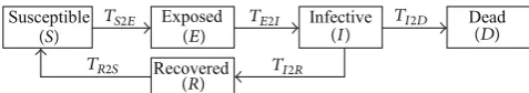
Susceptible Exposed Infective Dead

Recovered

(S) TS2E (E) TE2I (I) TI2D (D)

TR2S

[image:4.600.58.287.75.206.2]

(R) TI2R

Figure 2: The cycle of epidemic states.

instant𝑇EISR(𝑖). Suppose there are𝑁𝑁nodes in the network.

Then, for node 𝑖, there is a threshold 𝛽(𝑖) to determine

whether it is possible for the node to be infected by a certain

infective node and an amplifying factor𝛼(𝑖)to calculate the

initial energy when the node is infected. Basically, we can

assume all ripples have the same spreading speed𝑠and the

same energy decaying coefficient vector𝜂.

The second parameter group is epidemic specific. Because the nodes of network represent individuals, every node will

have a certain epidemic state at each time point. Let𝑆_𝑁(𝑖, 𝑡)

denote the epidemic state of node 𝑖at time 𝑡. Table 1 lists

the epidemic states used in this study.Figure 2shows how

an individual will go through these epidemic states in an epidemic cycle. Simply speaking, in the epidemic cycle, an individual is initially susceptible. Once s/he is infected, s/he becomes exposed and then s/he develops to be infective; an infected individual may either die or recover from the infection. A recovered individual usually gets postrecovery immunity. If this is temporary, then after a period of time of immunity, s/he will become susceptible again. As one can

see fromFigure 2, there is a time period for an individual to

transfer from one epidemic state to its followingup epidemic

state. Except 𝑇_𝑆2𝐸, all other state transfer times, that is,

𝑇𝐸2𝐼, 𝑇𝐼2𝐷, 𝑇𝐼2𝑅, and 𝑇𝑅2𝑆, are independent of the

ripple-spreading process, being instead mainly determined by the nature of the epidemic, the physical fitness of individuals, and/or relevant public health policies/measures. Basically, from statistical study of historical data, we may get an

esti-mate of each state transfer time distribution (excluding𝑇_𝑆2𝐸).

In this study, we assume they all have Poisson distributions.

For instance, 𝑇_𝐸2𝐼 may have a Poisson distribution with a

mean of𝑇_𝐸2𝐼. Therefore, with𝑇_𝐸2𝐼 as a parameter, we can

roughly know how long it will take for an individual to

transfer from state “𝐸” to state “𝐼”. When running the RSEM,

once a node becomes exposed, we then randomly assign a

𝑇_𝐸2𝐼to the node according to a Poisson distribution with𝑇_𝐸2𝐼

as the mean. Similarly, we deal with other state transfer times

except 𝑇_𝑆2𝐸. Therefore, in the second group, we have four

means as parameters, namely,𝑇_𝐸2𝐼,𝑇_𝐼2𝐷,𝑇_𝐼2𝑅, and𝑇_𝑅2𝑆. For

the sake of generality,𝑇_𝐸2𝐼, 𝑇_𝐼2𝐷, 𝑇_𝐼2𝑅, and𝑇_𝑅2𝑆are allowed

to be zero, which means one or more epidemic states may not be experienced by an individual in an epidemic cycle. For

example, if𝑇_𝐸2𝐼 = 0and𝑇_𝑅2𝑆 = 0, then there is no latency

period or postrecovery immunity.

Besides the two groups of parameters, there are three kinds of dynamics in the RSEM: the ripple-spreading process, the reaction of nodes to ripples, and the state transfer of nodes. The first two originate from the general work reported

(5)

are introduced. The dynamics of state transfer is a brand-new concept for the general ripple-spreading network model.

The ripple-spreading process in the RSEM is

mathemati-cally described as follows. Suppose ripple𝑖is associated with

the𝑖th node,𝑖 = 1, 2, . . . , 𝑁_𝑁. Then, let𝐸_𝑁(𝑖)be the initial

point energy of the ripple𝑖, 𝑒_𝑁(𝑖, 𝑡)the point energy of the

ripple𝑖at time𝑡, and𝑟_𝑁(𝑖, 𝑡)the radius of ripple𝑖. Initialize

𝐸𝑁(𝑖) = 0, 𝑒𝑁(𝑖, 0) = 0 and𝑟𝑁(𝑖, 0) = 0. Once ripple𝑖 is

triggered at a certain time point,𝐸_𝑁(𝑖)will be given a value

larger than zero. If𝐸_𝑁(𝑖) > 0and𝑆_𝑁(𝑖, 𝑡) =“𝐼” (i.e., the state

of node𝑖is “Infective”), then ripple𝑖will spread out as follows:

𝑟_𝑁(𝑖, 𝑡) = 𝑟_𝑁(𝑖, 𝑡 − 1) + 𝑠, (1)

𝑒_𝑁(𝑖, 𝑡) = 𝑓Decay(𝐸𝑁(𝑖) , 𝑟𝑁(𝑖, 𝑡)) , (2)

where 𝑓Decay is a function defining how the point energy

decays as the ripple spreads out. A typical decaying function may be

𝑓Decay(𝐸, 𝑟) = 𝜂 (𝑘) 𝐸_2𝜋𝑟 , (3)

and𝑘is an integer index calculated as

𝑘 = 𝑟𝑁(𝑖, 𝑡)_𝑠 . (4)

Once the𝑆_𝑁(𝑖, 𝑡)changes from “I” to “D” or “R”, reset𝐸_𝑁(𝑖) =

0, 𝑒_𝑁(𝑖, 0) = 0, and𝑟_𝑁(𝑖, 0) = 0.

The reaction of nodes to ripples defines how a node is

infected. Suppose node𝑖is reached by ripple𝑗at time𝑡; that

is,

𝑟_𝑁(𝑗, 𝑡) ≥ 𝐷_𝑁(𝑖, 𝑗) ≥ 𝑟_𝑁(𝑗, 𝑡 − 1) , (5)

where𝐷_𝑁(𝑖, 𝑗)is the distance between node𝑖and node𝑗. If

𝑆_𝑁(𝑖, 𝑡) =“𝑆” and𝑒_𝑁(𝑗, 𝑡) ≥ 𝛽(𝑖), that is, the point energy of

ripple𝑗is above the threshold of node𝑖, then node𝑖will be

infected with a probability which may be defined based on an

arctangent function of𝑒_𝑁(𝑗, 𝑡)as follows:

𝑝_𝑅(𝑖) = tan−1(𝜅 ((𝑒𝑁(𝑗, 𝑡) − 𝛽 (𝑖)) /𝛽 (𝑖)) − 𝛿) +_{𝜋/2 +} tan−1(𝛿)

tan−1(𝛿) ,

(6)

where 𝜅 > 0 and 𝛿 are coefficients which can adjust the

shape and location of the arctangent function. Once node𝑖

is infected, we establish a directional link from node𝑗 and

node𝑖by modifying the adjacency matrix:

𝑀_𝐴(𝑗, 𝑖) = 𝑀_𝐴(𝑗, 𝑖) + 1, (7)

set𝑆_𝑁(𝑖, 𝑡 + 1) =“𝐸”, set the initial point energy of ripple𝑖as

𝐸_𝑁(𝑖) = 𝛼 (𝑖) 𝑒_𝑁(𝑗, 𝑡) , (8)

record the time of becoming exposed𝑡_𝐸(𝑖) = 𝑡, and assign

values to 𝑇_𝐸2𝐼(𝑖), 𝑇_𝐼2𝐷(𝑖), 𝑇_𝐼2𝑅(𝑖), and 𝑇_𝑅2𝑆(𝑖) according to

relevant Poisson distributions defined by𝑇_𝐸2𝐼, 𝑇_𝐼2𝐷, 𝑇_𝐼2𝑅,

and𝑇_𝑅2𝑆.

Please note that, although ripple𝑖has𝐸_𝑁(𝑖) > 0at time

𝑡_𝐸(𝑖), it will not start spreading until the state of node𝑖has

become “Infective”, which is determined by the following

state transfer dynamics: if𝑆_𝑁(𝑖, 𝑡) = “𝐸” and 𝑡 − 𝑡_𝐸(𝑖) ≥

𝑇_𝐸2𝐼(𝑖), then set 𝑆_𝑁(𝑖, 𝑡 + 1) = “𝐼” and start the

ripple-spreading process for ripple𝑖; if𝑆_𝑁(𝑖, 𝑡) =“𝐼” and𝑡 − 𝑡_𝐸(𝑖) ≥

𝑇𝐸2𝐼(𝑖) + 𝑇𝐼2𝐷(𝑖), randomly decide whether node𝑖 will die

according to a preset death rate𝑅_𝐷; if node𝑖has died, set

𝑆_𝑁(𝑖, 𝑡 + 1) = “𝐷”, 𝑟_𝑁(𝑖, 𝑡) = 0, and𝐸_𝑁(𝑖) = 0, and stop

the ripple-spreading process of ripple𝑖; if𝑆_𝑁(𝑖, 𝑡) =“𝐼” and

𝑡 − 𝑡_𝐸(𝑖) ≥ 𝑇_𝐸2𝐼(𝑖) + 𝑇_𝐼2𝑅(𝑖), set𝑆_𝑁(𝑖, 𝑡 + 1) =“𝑅”, 𝑟_𝑁(𝑖, 𝑡) = 0, and𝐸_𝑁(𝑖) = 0, and stop the ripple-spreading process of ripple

𝑖; if𝑆_𝑁(𝑖, 𝑡) =“𝑅” and𝑡 − 𝑡_𝐸(𝑖) ≥ 𝑇_𝐸2𝐼(𝑖) + 𝑇_𝐼2𝑅(𝑖) + 𝑇_𝑅2𝑆(𝑖), set

𝑆_𝑁(𝑖, 𝑡 + 1) =“𝑆”. So, node𝑖has gone through an epidemic cycle.

By integrating the above parameters and dynamics, the proposed RSEM can be finally described as a whole by the following steps.

Step 1. Initialization, that is, set 𝑆_𝑁(𝑖, 0) = “𝑆”, 𝐸_𝑁(𝑖) =

0, 𝑟_𝑁(𝑖, 0) = 0, 𝑡 = 0and𝑀_𝐴(𝑗, 𝑖) = 0for all𝑖 = 1, 2, . . . ,

𝑁_𝑁 and 𝑗 = 1, 2, . . . , 𝑁_𝑁, randomly choose 𝑁EISR nodes

as initial cases, set their state as “E”, set their𝑇_𝐸2𝐼 as𝑇EISR,

and randomly set their 𝑇_𝐼2𝐷, 𝑇_𝐼2𝑅, and 𝑇_𝑅2𝑆 according to

the relevant Poisson distributions defined by𝑇_𝐼2𝐷,𝑇_𝐼2𝑅, and

𝑇_𝑅2𝑆.

Step 2. While the termination criteria are not satisfied, let𝑡 =

𝑡 + 1, do for𝑖 = 1, 2, . . . , 𝑁_𝑁.

Substep 2.1. Let𝑆_𝑁(𝑖, 𝑡) = 𝑆_𝑁(𝑖, 𝑡 − 1).

Substep 2.2. If𝐸_𝑁(𝑖) > 0and𝑆_𝑁(𝑖, 𝑡) =“𝐼”, let ripple𝑖spread for one time step by following the ripple-spreading process

described by (1) to (4).

Substep 2.3. If node𝑖has𝑆_𝑁(𝑖, 𝑡) =“𝑆” and is reached ripple𝑗

according to (5), calculate the reaction of node𝑖as described

by (6) to (8).

Substep 2.4. If 𝑆_𝑁(𝑖, 𝑡) ̸=“𝑆”, following the state transfer

dynamics to process node𝑖for one time step.

When an RSEM run is terminated, a network will appear based on all established directional links which indicate how the infectious disease has transmitted between individuals.

Figure 3illustrates how the infectious disease transmission can be simulated by the proposed RSEM.

2.3. Further Analysis of RSEM. As discussed in the Intro-duction section, social contacts and physical movements of individuals impose a big challenge to epidemic modeling. Fortunately, thanks to ripple-spreading dynamics, the pro-posed RSEM can effectively simulate the effect of social contacts and physical movements without actually applying such activities to each individual. Basically, the strength of social contacts and physical movements of an individual

is largely reflected by the amplifying factor 𝛼(𝑖) and the

(6)

(f). Node 2 has infected node 1; node 4 becomes infective.

EISR:1(I)

2(S)

3(S)

4(S)

2(S)

3(E)

4(S)

2(E)

3(I)

4(S)

EISR:1(S)

2(_I)

3(D)

4(E)

2(S)

3(I)

4(S)

2(I)

3(D)

4(_I)

EISR:1(I) EISR:1(R)

EISR:1(R)

EISR:1(_E)

(a). Node 1 is the initial case; other nodes are susceptible.

(b). Node 1 has infected node 3, which becomes exposed but not infective yet.

(c). Node 1 has recovered with temporary immunity; node 3 becomes infective.

(d). Node 3 has infected node 2 but failed to infect node 4. (e). Node 1 becomes

susceptible again; node 3 has died; node 2 becomes infective and

[image:6.600.70.531.69.351.2]

has infected node 4.

Figure 3: An illustration of RSEM.

likely to be infected, so s/he should have a smaller 𝛽(𝑖).

According to (6), one can see that a smaller 𝛽(𝑖)means a

higher probability of being infected. At the same time we set

a larger𝛼(𝑖)for a socially active individual, and, from (8), one

can see that his/her ripple will then have more point energy to

infect others, which is in line with the reality. According to (2)

and (3), as a ripple spreads out, its point energy decays, which

in general means that the infection probability becomes lower as the distance between two individuals increases. This is also the case in reality: for an individual, usually most of his/her social contacts and physical movements happen within a small group of people (compared with the whole community) and a limited physical space (compared with the entire space). Therefore, most secondary infections caused by him/her will be spatially limited. Now it is clear that, by associating the point energy of ripples to the probability of infection and the amplifying factor and the threshold of nodes to the social contacts and physical movements of individuals, the proposed RSEM provides a new approach to simulate and study the epidemic dynamic.

One may argue that, according to Table 1and Figure 2,

the proposed RSEM misses the state of “Admitted”, which usually means that individuals who are infective are quaran-tined in hospital and therefore have no chance to transmit the infection to others. Obviously, this state is not an original state in the natural epidemic cycle, but a man-made state due to the public health service. Actually, the effect of the

state of “Admitted” can be equivalent to shortening 𝑇_𝐼2𝐷

and𝑇_𝐼2𝑅, and increasing𝑇_𝑅2𝑆. Therefore, in this study, we do

not consider the state of “Admitted” explicitly. This will be further discussed later in the simulation section.

It should be noted that, in the ripple-spreading process,

(3) uses an energy decaying coefficient vector rather than

a single coefficient scalar. This is because the infectiousness over time after infection is not a constant, as shown by

the examples inFigure 4. Therefore, we can use a piecewise

function defined by the vector𝜂to describe the time-varying

infectiousness of a given epidemic.

In the reaction of node to ripples, according to (6), the

curve of the probability𝑝_𝑅(𝑖)for node𝑖to be infected has a

shape of an arctangent function like the solid line inFigure 5.

Basically, once𝑒_𝑁(𝑗, 𝑡) ≥ 𝛽(𝑖), the larger the point energy

𝑒𝑁(𝑗, 𝑡)is, the higher the probability for node𝑖to be infected

by node𝑗. The probability𝑝_𝑅(𝑖)does not go up linearly as

𝑒_𝑁(𝑗, 𝑡)increases. Actually,𝑝_𝑅(𝑖)increases very slowly before

𝑒_𝑁(𝑗, 𝑡)reaches a certain critical value, around which𝑝_𝑅(𝑖) goes up sharply and then gets almost saturated no matter

how large𝑒_𝑁(𝑗, 𝑡)is. This is reasonable, because, according to

(3), the value of𝑒_𝑁(𝑗, 𝑡)largely reflects the distance (spatial,

social, or both) between two nodes, and in reality infection occurs mainly within a certain range of spatial and/or social distance, whilst beyond that range the probability of infection

is quite low. The coefficient 𝜅determines how sharply the

probability curve changes around the critical value of𝑒_𝑁(𝑗, 𝑡):

the larger the value of𝜅, the sharper the probability curve.

The coefficient𝛿determines how likely it is that an𝑒_𝑁(𝑗, 𝑡)

will cause a large probability of infection: the smaller the

(7)

Time (hours)

In

fe

ct

io

u

sn

es

s

0 48 96 144 192

(a) Influenza A

In

fe

ct

io

u

sn

es

s

0 2 4 6 8 10

Time (hours)

(b) HIV-1

In

fe

ct

io

u

sn

es

s

0 10 20 30 40

Time (hours)

[image:7.600.79.523.72.227.2]

(c) Malaria

[image:7.600.50.292.268.633.2]

Figure 4: Biological infectiousness over time after infection for three different human pathogens [14].

Table 1: States used in epidemic model.

Symbol Epidemic state Description

𝑆 Susceptible Healthy Individuals who could potentially develop the disease.

𝐸 Exposed

Individuals who have been infected with the disease, but who are still in the latent period (with or without symptoms of the disease) and who cannot transmit the disease to others.

𝐼 Infective

Individuals who are infected with the disease (with or without symptoms of the disease) and who are capable of transmitting the infection to others.

𝑅 Recovered

Individuals who have recovered from infection thereby acquiring immunity (temporary or permanent) from infection.

𝐷 Dead Individuals who have died from

infection

0 0 1

𝛽(i) 𝛿 × 𝛽(i)/𝜅 + 𝛽(i)

Point energy of ripplej:e_N(j, t)

P

roba

b

ili

ty o

f no

de

i

b

ein

g inf

ec

ted

pR

(i)

Figure 5: Probability of infection and point energy of ripple.

the RSEM, one may sometimes use a piecewise probability

function, such as the dotted line inFigure 5, to approximate

the arctangent function.

From the description above, it is apparent that the proposed RSEM is more complicated than many existing

epidemic models. This also means that it is more flexible to modifications. For instance, the space where nodes distribute and ripples spread out is not necessarily the real geographic space. Instead, it can be an artificial multidimensional space which includes social relationships, shopping patterns, and habits. The nodes may not always be fixed; in other words, by referring to relevant statistic studies of long-distance travel-ling patterns, some randomly chosen nodes may occasionally jump in the space. The proposed RSEM can easily incorporate such modifications, but this is beyond the scope of this paper.

3. Genetic Algorithm for Tuning

Model Parameters

Like all other models, the proposed RSEM is supposed to be able to (i) simulate historic epidemic outbreaks, (ii) analyze epidemic dynamics/mechanism and health poli-cies/measures, and (iii) make forecasts to some extent. Simulating historic epidemic outbreaks is mainly used for model verification building confidence so that the model will be employed for analysis and forecasting. In the sim-ulation of historic epidemic outbreaks, the output of a model should match the relevant historic data as closely as possible. Basically, this can be assessed by comparing the

number of daily infections𝑁_𝐷𝐼(𝑡), the number of daily deaths

𝑁_𝐷𝐷(𝑡), the number of daily recoveries 𝑁_𝐷𝑅(𝑡), and the

basic reproduction ratio𝑅₀, which is defined as the average

number of secondary infections produced when one infected individual is introduced into a population where everyone

else is susceptible [14]. In short, the quantity 𝑅₀ governs

whether an infection can spread and be sustained within a

population. If 𝑅₀ is greater than one, then the number of

infections in a susceptible population will increase and the

infection will be sustained, whereas if𝑅₀is less than one, the

[image:7.600.51.292.284.513.2]

(8)

not impossible. Actually, the output of the RSEM does not simply rely on the values of parameters but is more determined by whether such values together satisfy certain

conditions, known or unknown. For instance, [21] derived

some conditions which involve all parameters to determine whether all nodes will be connected together in the general ripple-spreading network model. Such complicated relation-ships between parameters reflect the fact that in reality it is usual for many factors to work together in a complex, intermixed fashion. Tuning the parameters for a complicated model/system is often far beyond the capability of even human experts. Fortunately, we can turn to methods such as genetic algorithms (GAs) for help. A GA is a large-scale parallel stochastic searching and optimizing method inspired by the biological mechanisms of evolution and heredity. In recent years, GAs have been widely used for resolving various complex problems, particularly those including parameter

optimization [23–26]. The basic idea of a GA is that, given

a population of chromosomes, the environmental pressure causes natural selection (survival of the fittest), and hereby the fitness of the population grows. It is easy to see such a process as optimization. Given an objective function to be maximized, we can randomly create a set of candidate solutions (chromosomes) and use the objective function as an abstract fitness measure (the higher the better). Based on this fitness, some of the better chromosomes are chosen to seed the next generation by applying crossover and/or mutation. Crossover is applied to two selected chromosomes, the so-called parents, and results in one or two new chromosomes, the children. Mutation is applied to one chromosome and results in one new chromosome. Applying crossover and mutation leads to a set of new chromosomes, the offspring. Based on their fitness, these offsprings compete with the old chromosomes for a place in the next generation (in some GA implementations, the population is all replaced by the offspring). This process can be iterated until a solution is found or a previously set time limit is reached. Many components of such an evolutionary process are stochastic. According to Darwin, the emergence of new species, adapted to their environment, is a consequence of the interaction between the survival of the fittest mechanism and undirected variations. Variation operators must be stochastic, the choice of which pieces of information will be exchanged during crossover, as well as the changes in a chromosome during mutation, is random. On the other hand, selection operators can be either deterministic or stochastic. In the latter case fitter chromosomes have a higher chance of being selected than less fit ones, but typically even the weak chromosomes have a chance to become a parent or to survive. For more

theoretical details of GAs, readers may refer to [23–26].

To apply a GA in this study, firstly, we need to decide, in the RSEM, which parameters can be set up by hand and which ones need to be tuned by the GA. Basically, parameters

such as the number of initial cases𝑁EISR, the means of state

transfer times 𝑇_𝐸2𝐼, 𝑇_𝐼2𝐷, 𝑇_𝐼2𝑅, and𝑇_𝑅2𝑆, energy decaying

coefficient vector 𝜂, and death rate 𝑅_𝐷 can be easily set

up according to relevant historic data and statistic studies.

Coefficients𝜅and 𝛿can also be tuned by hand mainly to

change the overall shape of the infection probability curve as

shown inFigure 5. Most ripple-spreading related parameters

are purpose-designed and have no real-world meanings or references, and therefore they should be tuned by the GA. These parameters specifically include the initial point energy

𝐸EISR(𝑖) of initial cases, the ripple spreading speed 𝑠, the

threshold𝛽(𝑖), and the amplifying factor𝛼(𝑖). It should be

noted that we do not need to tune𝛽(𝑖) and 𝛼(𝑖)for every

node, but we just need to tune their means, that is, 𝛽and

𝛼, and then generate 𝛽(𝑖) and 𝛼(𝑖) according to a Poisson

distribution with𝛽and𝛼as the means, respectively.

Then, we construct a fitness function based on 𝑁_𝐷𝐼(𝑡),

𝑁_𝐷𝐷(𝑡),𝑁_𝐷𝑅(𝑡), and𝑅₀as follows:

𝐽 = 𝑤₁󵄨󵄨󵄨󵄨_󵄨𝑅₀− 𝑅∗

0󵄨󵄨󵄨󵄨_{󵄨 + 𝑤}2∑ 󵄨󵄨󵄨󵄨󵄨𝑁𝐷𝐼(𝑡) − 𝑁𝐷𝐼∗ (𝑡)󵄨󵄨󵄨󵄨_󵄨

+ 𝑤3∑ 󵄨󵄨󵄨󵄨󵄨𝑁𝐷𝐷(𝑡) − 𝑁𝐷𝐷∗ (𝑡)󵄨󵄨󵄨󵄨_󵄨

+ 𝑤4∑󵄨󵄨󵄨󵄨_󵄨𝑁𝐷𝑅(𝑡) − 𝑁𝐷𝑅∗ (𝑡)󵄨󵄨󵄨󵄨_{󵄨 ,}

(9)

where 𝑤₁ to𝑤₄ are weights, the variables with “∗” are the

approximated values of relevant historical data, and the over barred variables are the relevant mean results of a number of random RSEM runs with a given set of parameter values. Usually, the curve of historical data is not smooth and nor is the curve of a single RSEM run. If we directly compare the historical curve with the curve of any single RSEM run, the summed error will usually be very large, even though the two curves are actually similar to each other. Therefore, we need to use approximated values and average values, both of which are much smoother for accurate comparison. Another reason for utilizing the average results of many RSEM runs is that the proposed RSEM is stochastic in nature, which means that the model will deliver different results in different runs even for the same set of parameter values. Therefore, to better assess the effect of a given set of parameter values, a sufficient number of RSEM runs need to be conducted for a parameter value set.

Thus, we can use GA to tune the parameters for the RSEM as follows.

Step 1. Initialize a population of sets of parameter values.

Step 2. For a set of parameter values, conduct a number of RSEM runs, and then calculate the fitness based on the average results. Repeat the same for every set of parameter values in the population.

Step 3. If the termination criterion is satisfied, go toStep 4. Otherwise, perform selection, crossover, and mutation to generate a new population of sets of parameter values. Go to

Step 2.

Step 4. Output the best set of parameter values, and stop.

Once the RSEM is well tuned by the GA, we can then use it to analyze epidemic details and policy effects, as well as forecasting new trend or future development of an epidemic. Some relevant technical details concerning GA design and

(9)

however, that [22] focuses on applying a GA to optimize the

basic RSNM of [21] so as to generate small-world and

scale-free network topologies. As discussed inSection 2, the basic

RSNM is somewhat different from the RSEM proposed in this paper. Nevertheless, the use of a GA to optimize model

parameters in [22] is helpful to tune the RSEM in this paper.

4. Illustrative Simulation Results

As explained in Section 3, the first step in applying the

proposed RSEM is to use some historical data to tune the parameter values in order to simulate the associated real epidemic outbreak. Here we consider the March 2003 Severe Acute Respiratory Syndrome (SARS) outbreak in Hong Kong. From the empirical data for Hong Kong, we know that a severe localized epidemic occurred in Amoy Gardens. Through contact tracing, it has been estimated that 332 cases were involved in this outbreak, a large proportion of which could be traced to a single person. Outbreaks involving the direct spread of the disease from one primary case to a very large number of secondary cases are often referred to as “Super-Spreading Events”, which are often ideally used to test

epidemic models. As one can see from Figures6,7, and8, the

real historical data form no smooth curves. Because the SARS case in Amoy Gardens is a unique single case, we cannot get any smooth curve of average historical data, which makes it difficult to calculate the fitness of chromosome as defined

in (9). Thus, to be able to apply a GA to tune the reported

RSEM, we adopt the differential equations based model in

[20] to generate an approximated smooth curve of average

historical data. With 3 smooth curves (of daily infections,

death, and recovery, resp.) generated by the model in [20],

we can calculate the chromosome fitness according to (9) and

then apply GA to tune the RSEM parameters. It should be noted that there are actually no daily infection data, and we

hence use the daily admissions data in [20] to approximate

them. In this study, the weights𝑤₁ to𝑤₄ in (9) are set to

100, 1, 10, and 2, respectively. These values for𝑤₁to𝑤₄ are

chosen largely by referring to the data of basic reproduction ratio, daily admissions, daily death, and daily recovery in

[20], so that the four items in (9) will have roughly equal

contributions to the fitness function. In the test, all SARS-specific disease related parameters are set up according to

[20], and the number of nodes is 𝑁_𝑁 = 2396 (i.e., the

susceptible population in Amoy Gardens). For the GA, the crossover probability is set to 0.6, the mutation probability is set to 0.1, the population size is 200, and the number of evolving generations is 500. For each chromosome in a population, we use the parameter values represented by it to run the RSEM for 100 times, and then use the average results

to calculate its fitness according to (9). Finally, we use the

fittest chromosome in the last generation of GA to set the RSEM, in order to simulate the SARS case in Amoy Gardens.

Figures 6, 7, and 8 plot the final simulation results of

applying RSEM to study the SARS case in Amoy Gardens; the standard deviations (SDs) of the results of the model

in [20] and the RSEM from the historical data are given

in Table 2. From Figures 6, 7, and 8 and Table 2, one can see that (i) the average curves of RSEM are similar to those

of [20]; (ii) the SDs of the RSEM are close to those of

the model in [20]; (iii) the results of a single RSEM run

have patterns (peaks and valleys) fairly similar to those of historical data; (iv) the ranges and tendencies of RSEM data

all match those of historical data and [20]. Therefore, Figures

6, 7, and 8 and Table 2 illustrate that the proposed RSEM

and GA can deliver a fairly satisfactory performance in the case study of SARS and therefore can be useful to model epidemic dynamics. However, due to lack of relevant data on the physical fitness, immunity, and social activities of the population in Amoy Gardens, at the moment it is still difficult to explain or make sense of the values of RSEM parameters in this SARS case. Therefore, more cases studies based on different historical data and social survey data are still needed, which is beyond the scope of this paper and demands effort in future research.

Due to the early stage of this work, we have not collected sufficient historical data for parameter tuning purposes. However, we can still investigate the model based on synthetic data sets, in order to understand the properties of the model itself. Here, we can give some simulation results to see how the parameters can affect the output of the model. Now we set𝑁_𝑁 = 250; that is, the population of original susceptible individuals is 250. We assume there are 8 initial cases randomly distributed in the population. Firstly, we suppose that the population is uniformly randomly distributed in a

square area defined by coordinates (−1000,−1000) and (1000,

1000), and all initial cases have the same initial point energy

𝐸EISR = 10000, the Poisson means for generating 𝑇𝐸2𝐼(𝑖),

𝑇_𝐼2𝐷(𝑖), 𝑇_𝐼2𝑅(𝑖) and 𝑇_𝑅2𝑆(𝑖), 𝛽(𝑖) and 𝛼(𝑖) are 𝑇_𝐸2𝐼 = 10,

𝑇_𝐼2𝐷 = 15,𝑇_𝐼2𝑅 = 15and𝑇_𝑅2𝑆 = 20,𝛽 = 5, and𝛼 = 1000,

and coefficients𝜂 = 1, 𝜅 = 1, and𝛿 = 10. Then, in the

simulation, we want to study the influence of three sets of parameters: (i) the square area (which is related to the density

of population), (ii) the pair of𝛽and𝛼(which are related to

the overall social activeness of the population), and (iii) the

triple of𝑇_𝐼2𝐷,𝑇_𝐼2𝑅, and𝑇_𝑅2𝑆(which are related to the general

public health service standard). Each time we only change the value(s) of one set of parameters by 20% of the associated default values, while all the other parameters have the default

values as given above. Please note that𝛽 and 𝛼 change in

opposite directions (𝛽increases whilst𝛼decreases) and𝑇_𝑅2𝑆

and the pair of (𝑇_𝐼2𝐷, 𝑇_𝐼2𝑅) change in opposite directions

(𝑇_𝑅2𝑆increases whilst the other two decrease). For each given

whole set of parameter values, we conduct 10 RSEM runs. Then, we only check the number of total infections, and the

average results are given inTable 3, from which we have the

following observations.

(i) The default values for parameters result in a network where all nodes are connected, which means the whole population is eventually infected. This default case is used as a benchmark to assess the influence of some model parameters.

(10)

[image:10.600.47.550.95.147.2]

Table 2: Comparative results between RSEM and the model in [20].

Standard deviations Number of infections Number of death Number of recovery

Daily Cumulative Daily Cumulative Daily Cumulative

Model in [20] 12.7012 26.2656 1.5375 4.2721 7.9375 37.0366

RSEM 12.7217 27.2463 1.5573 3.5244 8.0686 40.9718

F eb 20 M ar ch 6 A p ri l 3 M ar ch 20 A p ri l 17 M ay 1 M ay 15 M ay 29 Date 0 20 40 60 80 100 120 140 160

Historical data A single RSEM run

Approximated curve in [20]

Average result of many RSEM runs

N u m b er o f da il y inf ec tio n s ( NDI ) (a) 0 200 400 600 800 1000 1200 1400 1600 1800 C u m u la ti ve n u m b er o f inf ec tio n s F eb 20 M ar ch 6 A p ri l 3 M ar ch 20 A p ri l 17 M ay 1 M ay 15 M ay 29 Date

[image:10.600.64.536.108.419.2]

(b)

Figure 6: Simulation results for Amoy Gardens, Hong Kong: number of infections.

0 2 4 6 8 10 12 14 N u m b er o f da il y de at h ( NDD ) F eb 20 M ar ch 6 A p ri l 3 M ar ch 20 A p ri l 17 M ay 1 M ay 15 M ay 29 Date

(a) 0 50 100 150 200 250 300 C u m u la ti ve n u m b er o f de at h F eb 20 M ar ch 6 A p ri l 3 M ar ch 20 A p ri l 17 M ay 1 M ay 15 M ay 29 Date

(b)

[image:10.600.71.529.461.712.2]

(11)

0 10 20 30 40 50 60 70

N

u

m

b

er o

f da

il

y r

eco

ve

ry

(

NDR

)

F

eb 20

M

ar

ch 6

A

p

ri

l 3

M

ar

ch 20

A

p

ri

l 17

M

ay 1

M

ay 15

M

ay 29

Date

(a)

0 200 400 600 800 1000 1200 1400

C

u

m

u

la

ti

ve

n

u

m

b

er o

f r

eco

ve

ry

F

eb 20

M

ar

ch 6

A

p

ri

l 3

M

ar

ch 20

A

p

ri

l 17

M

ay 1

M

ay 15

M

ay 29

Date

[image:11.600.69.530.73.322.2]

(b)

Figure 8: Simulation results for Amoy Gardens, Hong Kong: number of recovery.

(iii) Large threshold and small amplifying factor have a negative influence on the transmission of infectious diseases. This means a community where the overall social activeness is low will have a better resistance to epidemic outbreaks. When an 80% change applies to the default values, usually only the initial cases will cause a few infections, and the epidemic will die out soon.

(iv) Similarly, the general public health service standard plays a crucial role in the control of epidemic out-breaks. If infected individuals can be quarantined in

a timely manner, say, if𝑇_𝐼2𝐷and𝑇_𝐼2𝑅are reduced by

80%, then infections are largely limited to the initial cases and the nearby.

(v) The above simulation results clearly reveal the trends of the influence of different RSEM parameters. How-ever, again, to fully understand the performance of RSEM, extensive efforts are still needed based on various real epidemics data in future research.

5. Conclusions and Future Work

This paper reports a novel ripple-spreading network model for the study of infectious disease transmission. We term the new model the ripple-spreading epidemic model (RSEM). By mimicking the ripple-spreading phenomenon on a calm liquid surface, the new model has many natural advantages to describe spatial and temporal factors in the outbreak of plagues. The effect of individuals’ social activities, such as contacts and movements, which are often difficult for many existing models to simulate, can be effectively described by

Table 3: Influence of model parameters on total infections.

Change % default

values Square area (𝛽, 𝛼) (𝑇𝑅2𝑆, 𝑇𝐼2𝐷, 𝑇𝐼2𝑅)

0% 250.0 250.0 250.0

20% 228.7 219.3 232.5

40% 205.7 185.8 191.6

60% 136.4 108.2 93.8

80% 51.9 16.5 21.9

the amplifying factor of nodes and the point energy of ripples, which largely determines the probability of infection. As the point energy of a ripple decays as the ripple spreads out, the probability of infection decreases. The threshold of nodes is another important parameter determining the dynamic process of infectious disease transmission, and basically this parameter is well associated with the physical fitness and immunity of individuals. The proposed model is highly flexible to modifications and is therefore capable of incorporating new real factors which matter in the study of epidemic. The general model can be tuned by genetic algorithm according to the historic data of a specific plague, and the well-tuned model can then be used to analyze and forecast the associated infectious disease. The effectiveness of the proposed model and method is illustrated by some simulation results.

[image:11.600.309.547.389.481.2]

(12)

as a new epidemic model, the RSEM needs relevant data on the physical fitness, immunity, and social activities of the population in a community/society, in order to better set up and understand the RSRPs (ripple-spreading related param-eters). To get such data, a purpose-designed social survey needs to be conducted within a certain time window after a plague breaks out. Therefore, conducting relevant social survey for a recent plague event to collect sufficient data will be a crucial part of future work. Once such data are collected for a specific plague event, more comparisons with different relevant existing models will be made. Such application-oriented study needs to be conducted for different diseases, in order to explore the full potential of the proposed RSEM.

Conflict of Interests

The authors declare that there is no conflict of interests regarding the publication of this paper.

Acknowledgments

This work was supported in part by the China “973” Project under Grant 2012CB955404, the project Grant 2012-RC-02 from Beijing Normal University, China, and the Seventh Framework Programme (FP7) of the European Union under Grant PIOF-GA-2011-299725. Some early results of this paper

were presented at the2012 the 5th International Conference

on BioMedical Engineering and Informatics (BMEI 2012), October 16–18, 2012, Chongqing, China.

References

[1] H. Heesterbeek, “The law of mass-action in epidemiology: a historical perspective,” inEcological Paradigms Lost: Routes of

Theory Change, K. Cuddington and B. Beisner, Eds., pp. 81–105,

Elsevier, Burlington, Mass, USA, 2005.

[2] K. Dietz and J. A. P. Heesterbeek, “Daniel Bernoulli’s epidemio-logical model revisited,”Mathematical Biosciences, vol. 180, pp. 1–21, 2002.

[3] R. M. Anderson and R. M. May,Infectious Diseases of Humans:

Dynamics and Control, Oxford University Press, 1991.

[4] J. Glasser, M. Meltzer, and B. Levin, “Mathematical modeling and public policy: responding to health crises,” Emerging

Infectious Diseases, vol. 10, no. 11, pp. 2050–2051, 2004.

[5] R. M. May, “Uses and Abuses of Mathematics in Biology,”

Science, vol. 303, no. 5659, pp. 790–793, 2004.

[6] N. T. J. Bailey,The Mathematical Theory of Infectious Diseases

and Its Applications, Hafner Press, New York, NY, USA, 2nd

edition, 1975.

[7] C. I. Siettos and L. Russo, “Mathematical modeling of infectious disease dynamics,”Virulence, vol. 4, no. 4, pp. 295–306, 2013.

[8] P. D. O’Neill, “A tutorial introduction to Bayesian inference for stochastic epidemic models using Markov chain Monte Carlo methods,”Mathematical Biosciences, vol. 180, pp. 103–114, 2002.

[9] A. Kleczkowski and B. T. Grenfell, “Mean-field-type equations for spread of epidemics: the “small world” model,”Physica A, vol. 274, no. 1, pp. 355–360, 1999.

[10] “Computer simulation model provides tactics to deal with flu epidemic,” http://www.healthjockey.com/2009/05/04/compu-

ter-simulation-model-provides-tactics-to-deal-with-flu-epide-mic/.

[11] R. Connell, P. Dawson, and A. Skvortsov, “Comparison of an agent-based model of disease propagation with the generalised SIR epidemic model,” Tech. Rep. DSTO-TR-2342, 2009. [12] M. Toffoli,Cellular Automata Machines, Scientific

Computa-tion, MIT Press, Cambridge, Mass, USA, 1991.

[13] S. Boccaletti, V. Latora, Y. Moreno, M. Chavez, and D.-U. Hwang, “Complex networks: structure and dynamics,”Physics

Reports, vol. 424, no. 4-5, pp. 175–308, 2006.

[14] N. C. Grassly and C. Fraser, “Mathematical models of infectious disease transmission,”Nature Reviews Microbiology, vol. 6, no. 6, pp. 477–487, 2008.

[15] R. Pastor-Satorras and A. Vespignani, “Epidemic spreading in scale-free networks,”Physical Review Letters, vol. 86, no. 14, pp. 3200–3203, 2001.

[16] A. I. Reppas, K. G. Spiliotis, and C. I. Siettos, “Epidemionics: from the host-host interactions to the systematic analysis of the emergent macroscopic dynamics of epidemic networks,”

Virulence, vol. 1, no. 4, pp. 338–349, 2010.

[17] R. Breban, R. Vardavas, and S. Blower, “Linking population-level models with growing networks: a class of epidemic models,”Physical Review E, vol. 72, no. 4, part 2, Article ID 046110, p. 8, 2005.

[18] M. J. Keeling and K. T. D. Eames, “Networks and epidemic models,”Journal of the Royal Society Interface, vol. 2, no. 4, pp. 295–307, 2005.

[19] D. Helbing, “Globally networked risks and how to respond,”

Nature, vol. 497, pp. 51–59, 2013.

[20] N. Jia and L. Tsui, “Epidemic modelling using SARS as a case study,”North American Actuarial Journal, vol. 9, no. 4, pp. 28– 42, 2005.

[21] X.-B. Hu, M. Wang, M. S. Leeson, E. L. Hines, and E. Di Paolo, “Deterministic ripple-spreading model for complex networks,”

Physical Review E, vol. 83, no. 4, Article ID 046123, 2011.

[22] X. B. Hu, M. Wang, and M. S. Leeson, “Ripple-spreading net-work model optimization by genetic algorithm,”Mathematical

Problems in Engineering, vol. 2013, Article ID 176206, 15 pages,

2013.

[23] J. H. Holland, Adaptation in Natural and Artificial Systems, University of Michigan Press, Ann Arbor, Mich, USA, 1975. [24] E. Goldberg, Genetic Algorithms in Search Optimization &

Machine Learning, Addison-Wesley, Reading, Mass, USA, 1989.

[25] Z. Michalewicz,Genetic Algorithms + Data Structures =

Evolu-tion Programs, Springer, Berlin, Germany, 2nd edition, 1994.

[26] A. E. Eiben and J. E. Smith,Introduction to Evolutionary

Com-puting, Natural Computing Series, Springer, Berlin, Germany,

(13)

Submit your manuscripts at

http://www.hindawi.com

Operations

Research

Advances in

Hindawi Publishing Corporation

http://www.hindawi.com Volume 2013

http://www.hindawi.com Volume 2013 Mathematical Problems in Engineering

Abstract and Applied Analysis

ISRN

Applied Mathematics

International Journal of

Combinatorics

http://www.hindawi.com Volume 2013 Journal of Function Spaces and Applications

International Journal of Mathematics and Mathematical Sciences

Hindawi Publishing Corporation http://www.hindawi.com Volume 2013

ISRN

Geometry Hindawi Publishing Corporation

Discrete Dynamics in Nature and Society

http://www.hindawi.com Volume 2013 Advances in

Mathematical Physics

ISRN Algebra

Probability

and

Statistics

Journal of

ISRN

Mathematical Analysis

Journal of

Applied Mathematics

Sciences

Stochastic Analysis

International Journal of Hindawi Publishing Corporation

http://www.hindawi.com Volume 2013 Hindawi Publishing Corporation

The Scientific

World Journal

ISRN

Discrete Mathematics

Hindawi Publishing Corporation http://www.hindawi.com

Differential Equations International Journal of