http://wrap.warwick.ac.uk
Original citation:
Dedner, Andreas, Madhavan, P. and Stinner, Björn. (2013) Analysis of the discontinuous
Galerkin method for elliptic problems on surfaces. IMA Journal of Numerical Analysis,
Volume 33 (Number 3). ISSN 0272-4979
Permanent WRAP url:
http://wrap.warwick.ac.uk/57150
Copyright and reuse:
The Warwick Research Archive Portal (WRAP) makes this work by researchers of the
University of Warwick available open access under the following conditions. Copyright ©
and all moral rights to the version of the paper presented here belong to the individual
author(s) and/or other copyright owners. To the extent reasonable and practicable the
material made available in WRAP has been checked for eligibility before being made
available.
Copies of full items can be used for personal research or study, educational, or
not-for-profit purposes without prior permission or charge. Provided that the authors, title and
full bibliographic details are credited, a hyperlink and/or URL is given for the original
metadata page and the content is not changed in any way.
Publisher’s statement:
This is a pre-copyedited, author-produced PDF of an article accepted for publication in
IMA Journal of Numerical Analysis following peer review. The definitive
publisher-authenticated version Dedner, Andreas, Madhavan, P. and Stinner, Björn. (2013)
Analysis of the discontinuous Galerkin method for elliptic problems on surfaces. IMA
Journal of Numerical Analysis, Volume 33 (Number 3). ISSN 0272-4979 is available
online at:
http://dx.doi.org/10.1093/imanum/drs033
A note on versions:
The version presented here may differ from the published version or, version of record, if
you wish to cite this item you are advised to consult the publisher’s version. Please see
the ‘permanent WRAP url’ above for details on accessing the published version and note
that access may require a subscription.
surfaces
ANDREASDEDNER, PRAVINMADHAVAN ANDBJORN¨ STINNER Mathematics Institute and Centre for Scientific Computing, University of Warwick,
Coventry CV4 7AL, UK
We extend the discontinuous Galerkin (DG) framework to a linear second-order elliptic problem on a compact smooth connected and oriented surface inR3. An interior penalty (IP) method is introduced on
a discrete surface and we derive a-priori error estimates by relating the latter to the original surface via the lift introduced in Dziuk (1988). The estimates suggest that the geometric error terms arising from the surface discretisation do not affect the overall convergence rate of the IP method when using linear ansatz functions. This is then verified numerically for a number of test problems. An intricate issue is the approximation of the surface conormal required in the IP formulation, choices of which are investigated numerically. Furthermore, we present a generic implementation of test problems on surfaces.
Keywords: discontinuous galerkin; interior penalty; surface partial differential equations; error analysis.
1. Introduction
Partial differential equations (PDEs) on manifolds have become an active area of research in recent years due to the fact that, in many applications, models have to be formulated not on a flat Euclidean domain but on a curved surface. For example, they arise naturally in fluid dynamics (e.g. surface active agents on the interface between two fluids, James & Lowengrub (2004)) and material science (e.g. diffusion of
species along grain boundaries, Deckelnicket al.(2001)) but have also emerged in areas as diverse as
image processing and cell biology (e.g. cell motility involving processes on the cell membrane, Neilson
et al.(2011) or phase separation on biomembranes, Elliott & Stinner (2010)).
Finite element methods (FEM) for elliptic problems and their error analysis have been successfully applied to problems on surfaces via the intrinsic approach in Dziuk (1988) based on interpolating the surface by a triangulated one. This approach has subsequently been extended to parabolic problems in Dziuk & Elliott (2007a) as well as evolving surfaces in Dziuk & Elliott (2007b). Ju & Du (2009) and Giesselmann & M¨uller (2013) have also considered finite volume methods on surfaces via the intrinsic approach. However, as in the planar case there are a number of situations where FEM may not be the appropriate numerical method, for instance, advection dominated problems which lead to steep gradients or even discontinuities in the solution.
DG methods are a class of numerical methods that have been successfully applied to hyperbolic, elliptic and parabolic PDEs arising from a wide range of applications. Some of its main advantages compared to ‘standard’ finite element methods include the ability of capturing discontinuities as arising in advection dominated problems, and less restriction on grid structure and refinement as well as on the choice of basis functions. The main idea of DG methods is not to require continuity of the solution between elements. Instead, inter-element behaviour has to be prescribed carefully in such a way that the resulting scheme has adequate consistency, stability and accuracy properties. A short introduction to DG methods for both ODEs and PDEs is given in Cockburn (2003). A history of the development
of DG methods can be found in Cockburnet al.(2000) and Arnoldet al.(2002). Arnoldet al.(2002)
provides an in-depth analysis of a large class of discontinuous Galerkin methods for second-order elliptic
problems.
The motivation of this study has been to investigate the issues arising when attempting to apply DG methods to problems on surfaces. We restrict our analysis to a linear second-order elliptic PDE on a compact smooth connected and oriented surface. We expect that parabolic problems on evolving surfaces as featured in the above mentioned applications can be dealt with along the lines of Dziuk & Elliott (2007b).
This paper is organised in the following way. We consider a second-order elliptic equation on a
compact smooth connected and oriented surfaceΓ ⊂R3and introduce a particular DG method known
as the interior penalty (IP) method on a triangulated surfaceΓh. The surface IP method we consider
is similar in nature to the one introduced in Arnold (1982), and its well-posedness follows naturally
from results in the planar case given in Arnoldet al.(2002) and Ainsworth & Rankin (2011). We then
derive a-priori error estimates in the appropriate norms by relatingΓhtoΓ via a lifting operator and by
making use of results from Dziuk (1988) and Giesselmann & M¨uller (2013) to show that the additional geometric error terms arising when approximating the surface scale in such a way that they do not affect the convergence rates proved and observed for the standard FEM approach in Dziuk (1988) when using linear ansatz functions.
We then present some numerical results, making use of the Distributed and Unified Numerics
Envi-ronment (DUNE) software package (see Bastianet al.(2008b), Bastianet al.(2008a)) and, in particular,
the DUNE-FEM module described in Dedneret al.(2010) (also see dune.mathematik.uni-freiburg.de
for more details on this module). We consider a number of test problems, for which we compute
ex-perimental orders of convergence (EOCs) in both theL2norm and theDGnorm, and show that these
coincide with the theoretical error estimates derived in the previous section. Furthermore, we consider several intuitive ways of approximating the surface conormal in our IP formulation, and investigate the resulting schemes numerically. In the process, we present a generic implementation of test problems on surfaces which follows as a direct application of the Demlow & Dziuk (2008) algorithms.
Finally, we briefly present numerical results for nonconforming grids and higher order polynomial ansatz functions, which suggest that the convergence rates of the standard FEM approach still hold for such generalisations.
2. Notation and Setting
The notation in this section closely follows the one used in Dziuk (1988). LetΓ be a compact smooth
connected and oriented surface inR3. For simplicity, we assume that∂ Γ =/0. Letd denote the signed
distance function toΓ which we assume to be well-defined in a sufficiently thin open tubeUaroundΓ.
The orientation ofΓ is set by taking the normalνofΓ to be in the direction of increasingdwhence
ν(ξ) =∇d(ξ), ξ∈Γ.
With a slight abuse of notation we also denote the projection toΓ byξ, i.e.ξ :U→Γ is given by
ξ(x) =x−d(x)ν(x) whereν(x):=ν(ξ(x)). (2.1)
Later on, we will consider a triangulated surfaceΓh⊂UapproximatingΓsuch that there is a one-to-one
relation between pointsx∈Γhandξ ∈Γ so that, in particular, the above relation (2.1) can be inverted.
Throughout this paper, we denote by
the projection onto the tangent spaceTξΓ onΓ at a pointξ ∈Γ. Here⊗denotes the usual tensor
product.
DEFINITION2.1 For any functionη defined on an open subset ofU containingΓ we can define its
tangential gradientonΓ by
∇Γη:=∇η−(∇η·ν)ν=P∇η
and then theLaplace-Beltramioperator onΓ by
∆Γη:=∇Γ·(∇Γη).
DEFINITION2.2 We define the surface Sobolev spaces
Hm(Γ):={u∈L2(Γ) : Dαu∈L2(
Γ)∀|α|6m}, m∈N∪ {0},
with corresponding Sobolev seminorm and norm respectively given by
|u|Hm(Γ):=
∑
|α|=mkDαuk2
L2(Γ)
!1/2
, kukHm(Γ):=
m
∑
k=0
|u|2Hk(Γ)
!1/2
.
We refer to Wloka (1987) for a proper discussion of Sobolev spaces on manifolds. The problem that we consider in this paper is the following second-order elliptic equation:
−∆Γu+u=f (2.2)
for a given f ∈L2(Γ). Using integration by parts on surfaces the weak problem reads:
PΓ
Findu∈H1(Γ)such that
Z
Γ
∇Γu·∇Γv+uv dA=
Z
Γ
f v dA ∀v∈H1(Γ). (2.3)
Existence and uniqueness of a solutionufollows from standard arguments. We assume thatu∈H2(Γ)
satisfies
kukH2(Γ)6CkfkL2(Γ) (2.4)
where we refer to Aubin (1982) and Wloka (1987) for more details on elliptic regularity on surfaces.
3. Approximation and Properties
To obtain a discretisation ofu, the smooth surfaceΓ is approximated by a polyhedral surfaceΓh⊂U
composed of planar triangles. LetThbe the associated regular, conforming triangulation ofΓhi.e.
Γh=
[
Kh∈Th
Kh.
The vertices are taken to sit onΓ so thatΓhis its linear interpolation. We assume that the projection map
ξ defined in (2.1) is a bijection when restricted toΓh, thus avoiding multiple coverings ofΓ byΓh. Let
Ehdenote the set of all codimension one intersections of elementsKh+,K
−
define the conormaln+h on such an intersectioneh∈Ehof elementsKh+andK
−
h by demanding that
•n+h is a unit vector,
•n+h is tangential to (the planar triangle)Kh+,
•in each pointx∈ehwe have thatn+h·(y−x)60 for ally∈K
+
h.
Analogously one can define the conormaln−h onehby exchangingKh+withK
−
h. A discrete DG space
associated withΓhis given by
Vh:={vh∈L2(Γh) : vh|Kh ∈P 1(K
h)∀Kh∈Th}
i.e. the space of piecewise linear functions which are globally inL2(Γh). Forvh∈Vh, let
v+h/−:=vh ∂Kh+/−.
We can now define a discrete DG formulation onΓhfor a given function fh∈L2(Γh)(note that, in
gen-eral, this is not a finite element function, it will be related to the function f given in problem(PΓ)later
on, see (3.5) below):
PIP
Γh
Finduh∈Vhsuch that
aIPΓ
h(uh,vh) =
∑
Kh∈Th Z
Kh
fhvhdAh∀vh∈Vh (3.1)
where
aIPΓ
h(uh,vh):=
∑
Kh∈Th Z
Kh
∇Γhuh·∇Γhvh+uhvhdAh
−
∑
eh∈Eh Z
eh
(u+h −u−h)1
2(∇Γhv
+
h·n
+
h−∇Γhv −
h ·n
−
h) + (v
+
h−v
−
h)
1 2(∇Γhu
+
h·n
+
h−∇Γhu −
h·n
−
h)dsh
+
∑
eh∈EhZ
eh
βeh(u
+
h−u
−
h)(v
+
h−v
−
h)dsh. (3.2)
The penalty parametersβeh are given byβeh=ωehh
−1
eh whereheh is some length scale associated with
the intersectioneh(for instance, the edge length). The interior penalty parametersωeh are uniformly
bounded with respect toh:=maxeh∈Ehheh.
REMARK3.1 This formulation corresponds to the one found in Arnoldet al.(2002) in the case when the domain is flat and is similar in nature to the original formulation of the IP method found in Arnold
(1982) for which the conormalsn+h/−are associated with their respective gradient terms rather than the
scalar terms. It is important to point out that this formulation is not equivalent to using the formulation
found in Arnoldet al.(2002) onΓh. We will discuss this issue further in Section 5.
We now define a norm on the space of piecewise smooth functions:
DEFINITION3.1 Foruh∈Vhwe define
|uh|21,h:=
∑
Kh∈Thkuhk2H1(K
h) , |u| 2
∗,h:=
∑
eh∈Ehh−1e
h ku
+
h −u
−
hk
2
L2(e
The DG norm is given by
kuhk2DG:=|uh|12,h+|uh|2∗,h.
LEMMA3.1 LetEKh denote the set containing the individual edges of elementKh. Then ifβeh=ωehh
−1
eh with
ωeh > max
Kh∈Th:
eh⊂∂Kh 1 2e˜
∑
h∈EKh
|e˜h|2 |Kh|
for all eh∈Eh, (3.3)
thenaΓIP
h is stable and bounded. Hence there is a unique solutionuh∈Vhof(P
IP
Γh)which satisfies
kuhkDG6CkfhkL2(Γ
h). (3.4)
Proof. Boundedness and stability of (3.2) follow in a similar way as for the classical IP method (see
Arnoldet al.(2002) for more details) since all the arguments apply toΓh. For the lower bound of the
penalty parameters, the proof of Lemma 2.1 in Ainsworth & Rankin (2011) applies straightforwardly
to the surfaceΓh. Note that the reason why these results naturally extend ontoΓhis that the latter is
composed of planar triangles. By Lax-Milgram, the uniqueness property follows.
Our goal now is to compare the solutionu∈H2(Γ)of(PΓ)with the solutionuh∈Vhof(PΓIPh)but these functions are defined on different domains. The approach suggested in Dziuk (1988) is to lift
functions defined on the discrete surfaceΓhonto the smooth surfaceΓ.
DEFINITION3.2 For any functionwdefined onΓhwe define theliftontoΓ by
wl(ξ):=w(x(ξ)), ξ∈Γ,
where by (2.1) and the non-overlapping of the triangular elements,x(ξ)is defined as the unique solution
of
x=ξ+d(x)ν(ξ).
Extending wl constantly along the liness7→ξ+sν(ξ)we obtain a function defined onU. In
particular, we
define fhsuch that fhl=f onΓ. (3.5)
By (2.1), for everyKh∈Th, there is a unique curved triangleKhl :=ξ(Kh)⊂Γ. Note that we assumed
ξ(x)is a bijection so multiple coverings are not permitted. We now define the regular, conforming
triangulationTl
h ofΓ such that
Γ= [ Kl
h∈Thl
Khl.
The triangulationThl ofΓ is thus induced by the triangulationThofΓhvia the lift. Similarly,elh:=
ξ(eh)∈Ehlare the unique curved edges.
The appropriate function space for lifted functions is given by
Vhl:={vhl ∈L2(Γ) : vhl(ξ) =vh(x(ξ))with somevh∈Vh}.
Note that the DG norm for functionsulh∈Vhlis the same one as in Definition 3.1 but with the
triangula-tionTl
h instead and corresponding length scalehel
h
associated withelh. The context of its use makes it
clear which DG norm we are dealing with. Furthermore, we observe that
hle
since the deformation of the straight edges can only increase their length. We now prove some geometric
error estimates relatingΓ toΓh.
LEMMA3.2 LetΓ be a compact smooth connected and oriented surface inR3andΓhits linear
inter-polation with outward unit normalνh. LetH=∇2d andPh=I−νh⊗νh. Furthermore, we denote
byδhthe local area deformation when transformingKhtoKhl i.e. δhdAh=dAandδeh the local edge
deformation when transformingehtoelhi.e.δehdsh=ds. Then we have
kdkL∞(Γ)6Ch2, k1−δhkL∞(Γ)6Ch2,kν−νhkL∞(Γ)6Ch, kP−RhkL∞(Γ)6Ch2
k1−δehkL∞(Γ)6Ch2,kP−RehkL∞(Γ)6Ch2andkn−PnlhkL∞(el h)6Ch
2
whereRh:=δ1
hP(I−dH)Ph(I−dH)andReh:= 1
δehP(I−dH)Ph(I−dH).
Proof. All these geometric estimates follow from standard interpolation theory via the linear
interpola-tion ofΓ. Proofs of the first four estimates can be found in Dziuk (1988), the fifth (and thus sixth) one
in Giesselmann & M¨uller (2013). The last estimate is a corollary of another result in Giesselmann &
M¨uller (2013), which states that ifnandnlhare given as before andτdenotes a unit tangent vector on
someelh∈El
h, we have
|(τ,nlh)|6Ch2,|1−(n,nlh)|6Ch2.
WritingPnlh= (τ,Pnlh)τ+ (n,Pnlh)n, we deduce that indeed
kn−PnlhkL∞(el h)
=kn−(τ,Pnlh)τ−(n,Pnlh)nkL∞(el h)
6|1−(n,Pnlh)|+|(τ,Pnlh)|=|1−(n,nlh)|+|(τ,nlh)|=O(h2).
LEMMA3.3 Letuh∈Vhsatisfy (3.4). Thenulh∈Vhlsatisfies
kulhkDG6CkfkL2(Γ) (3.7)
for sufficiently smallh.
Proof. We first show that that for any functionvh∈Vh,
kvhkDG>CkvlhkDG. (3.8)
The|·|2
1,hcomponent of the DG norm is dealt with in exactly the same way as in Dziuk (1988). Similarly,
making use of Lemma 3.2 and the fact thath−1e
h >h −1
el h
(see (3.6)), we obtain the following for the| · |2 ∗,h
component of the DG norm:
∑
eh∈Eh
h−1e
h Z
eh
(v+h −v−h)2dsh>
∑
elh∈Elh
h−1
elh
Z
el h
(vlh+−vlh−)2 1
δeh
ds
=
∑
elh∈Ehl
h−1
el h
Z
elh
(vlh+−vlh−)2ds+
∑
elh∈Ehl
h−1
el h
Z
elh
(vlh+−vlh−)2
1
δeh
−1
ds
> 1−Ch2
∑
elh∈El h
h−1
elh
Z
el h
which yields the desired estimate for sufficiently small h. Noting that kfhkL2(Γ
h) 6Ckf
l
hkL2(Γ) =
CkfkL2(Γ)(see Dziuk (1988)), we can extend the stability estimate (3.4) to the lifted discrete function
ulhas required.
We now define a bilinear form onΓ induced byaIPΓ
h and the lifting operator:
aIPΓ(u,v):=
∑
Khl∈Tlh Z
Kl h
∇Γu·∇Γv+uv dA
−
∑
elh∈El h Z
el h
(u+−u−)1
2(∇Γv
+·n+− ∇Γv
−
·n−) + (v+−v−)1
2(∇Γu
+·n+− ∇Γu
−
·n−)ds
+
∑
elh∈Ehl Z
elh βel
h(u
+−u−)(v+−v−)ds (3.9)
wheren+andn−are respectively the unit surface conormals toKhl+andKhl−onel
h∈Ehland the penalty
parameters are defined to beβel
h :=βeh
δeh. This bilinear form is well defined for functionsu,v∈H
2(Γ) +
Vhl, and since the weak solutionugiven by (2.3) is inH2(Γ)it satisfies
aIPΓ(u,v) =
∑
Khl∈Tlh Z
Khl
f v dA ∀v∈H2(Γ) +Vhl. (3.10)
We now state and prove a technical estimate of importance for boundedness and stability ofaΓIP.
LEMMA3.4 Letw∈H2(Γ)andwlh∈Vhl. Then for sufficiently smallh,
k∇Γ(w+wlh)k
2
L2(∂Kl h)6
C
1
hk∇Γ(w+w
l h)k
2
L2(Kl h)
+hkwk2 H2(Kl
h)
. (3.11)
Proof. We define ˜wandwhsuch that their lifts coincide withwandwlh, respectively. Since ˜w+wh∈
H2(Kh)on eachKh, applying the trace theorem and a standard scaling argument onKh∈Thyields
Z
∂Kh
|∇Γh(w˜+wh)| 2ds
h6C
1
h Z
Kh
|∇Γh(w˜+wh)| 2dA
h+h
Z
Kh
|∇2Γ
hw˜| 2dA
h
where we used that∇2Γ
hwh=0 thanks to the linearity of the finite element functions. Lifting the estimate
ontoΓ and making use of estimate (2.17) in Demlow (2009), we have
Z
∂Khl
∇Γ(w+wlh)·Reh∇Γ(w+wlh)ds6C
1
h Z
Khl
|∇Γ(w+wlh)|2dA+h
Z
Klh
|∇2Γw|2+|∇Γw|2dA
whereReh is given as in Lemma 3.2. We thus obtain
1−Ch2
Z
∂Kl h
|∇Γ(w+w
l h)|
2ds 6C 1 h Z Kl h
|∇Γ(w+w
l h)|
2dA+hZ
Kl h
|∇Γ2w|2+|∇Γw|
2dA
Following the lines of Arnoldet al.(2002) along with Lemma 3.4, we can show the boundedness estimate
aΓIP(w+wlh,vlh)6Cblkw+wlhkDG+h2kwkH2(Γ)
kvlhkDG for all w∈H2(Γ),wlh,vlh∈Vhl, (3.12)
and the stability estimate
aIPΓ(wlh,wlh)>Clskwlhk2
DG for all wlh∈Vhl. (3.13)
4. Convergence
THEOREM4.1 Letu∈H2(Γ)anduh∈Vhdenote the solutions to(PΓ)and(PIPΓh), respectively. Denote
byulh∈Vhlthe lift ofuhontoΓ. Then
ku−ulhkL2(Γ)+hku−ulhkDG6Ch2kfkL2(Γ).
The proof will follow an argument similar to the one outlined in Arnoldet al.(2002). Using the
stability result (3.13), we have
kφhl−ulhk2DG6 1
Cl s
aIPΓ(φhl−uhl,φhl−ulh) = 1
Cl s
aIPΓ(u−ulh,φhl−ulh) + 1
Cl s
aIPΓ(φhl−u,φhl−ulh) (4.1)
whereφhl ∈Vhl. Since we do not directly have Galerkin orthogonality the first term is not zero, and the
second term will require an interpolation estimate. These terms are addressed by the following lemmas:
LEMMA4.1 For a givenw∈H2(Γ)there exists an interpolantIhlw∈Vhl such that
kw−IhlwkL2(Γ)+hk∇Γ(w−Ihlw)kL2(Γ)6Ch2
k∇2ΓwkL2(Γ)+hk∇ΓwkL2(Γ)
.
Proof. See Dziuk (1988).
LEMMA4.2 Letuandulhbe given as in Theorem 4.1 and define the functionalEhonVhlby
Eh(vlh):=a IP
Γ(u−u
l h,v
l h).
ThenEhcan be written as
Eh(vlh) =
∑
Khl∈Tlh Z
Kl h
(Rh−P)∇Γu
l h·∇Γv
l h+ 1 δh −1
ulhvlh+
1− 1
δh
f vlhdA
+
∑
elh∈Elh Z
el h
(ulh+−ulh−)1
2(∇Γv
l+
h ·n
+− ∇Γv
l−
h ·n
−
)
−(ulh+−ulh−)1
2(P
+
h(I−dH)P∇Γv
l+
h ·n l+
h −P
−
h(I−dH)P∇Γv
l−
h ·n l−
h )
1
δeh
ds
+
∑
elh∈Elh Z
el h
(vlh+−vlh−)1
2(∇Γu
l+
h ·n
+− ∇Γu
l−
h ·n
−
)
−(vlh+−vlh−)1
2(P
+
h(I−dH)P∇Γu
l+
h ·n l+
h −P
−
h (I−dH)P∇Γu
l−
h ·n l−
h )
1
δeh
whereRhis given as in Lemma 3.2. Furthermore,Ehscales quadratically inhi.e.
|Eh(vlh)|6Ch2kfkL2(Γ)kvlhkDG. (4.2)
REMARK4.1 Note that the error functionalEhin Lemma 4.2 includes all of the terms of the classical
FEM setting (see Dziuk (1988)) as well as additional terms arising from the jumps across elements which characterise the DG method.
The proof of Lemma 4.2 will be the main part of this section. Before we give its full proof, we will complete that of Theorem 4.1 assuming this result. Using the estimate (4.1) given at the start of the proof of Theorem 4.1, the boundedness result (3.12), the elliptic regularity result (2.4) and the quadratic
scaling ofEhinh(4.2), we have
kφl
h−ulhk2DG6
1
Cl s
Eh(φhl−ulh) +
1
Cl s
aΓIP(φhl−u,φhl−ulh)
6 1 Cl s
Eh(φhl−ulh) +C l b Cl s kφl
h−ukDG+h2kukH2(Γ)
kφl
h−ulhkDG
6Ch2kfkL2(Γ)kφhl−ulhkDG+C
kφl
h−ukDG+h2kfkL2(Γ)
kφl
h−ulhkDG,
thus
kφhl−ulhkDG6Ch2kfkL2(Γ)+Ckφhl−ukDG.
Now taking the continuous interpolantφhl=Ihluand using Lemma 4.1 we obtain
ku−ulhkDG6ku−φhlkDG+kφhl−ulhkDG6ku−φhlkDG+Ch2kfkL2(Γ)+Ckφhl−ukDG6ChkfkL2(Γ)
as required. TheL2error estimate can be derived using the usual Aubin-Nitsche trick in a similar way
as in Dziuk (1988), which concludes the proof of Theorem 4.1.
Proof of Lemma 4.2. The expression for the error functionalEhgiven in Lemma 4.2 is obtained by
considering the difference between the two equations (3.10) and (3.1). In order to do this, the integrals
of (3.1) have to first be lifted ontoΓ. For everyKh∈Th, we have
Z
Kh
∇Γhuh·∇Γhvh+uhvhdAh= Z
Klh
Rh∇Γulh·∇Γvlh+
1
δh
ulhvlhdA.
Furthermore, for everyeh∈Eh, we have
Z
eh
(u+h −u−h)1
2(∇Γhv
+
h·n
+
h −∇Γhv −
h·n
−
h) + (v
+
h−v
−
h)
1 2(∇Γhu
+
h·n
+
h−∇Γhu −
h ·n
−
h)dsh
=
Z
elh
(ulh+−ulh−)1
2(P
+
h (I−dH)P∇Γvhl+·nlh+−P
−
h(I−dH)P∇Γvl
−
h ·n l−
h )
+ (vlh+−vlh−)1
2(P
+
h (I−dH)P∇Γuhl+·nlh+−P
−
h(I−dH)P∇Γul
−
h ·n l−
h )
1
δeh
ds.
And finally, we have usingβel
h
=βeh
δeh that
Z
eh
βeh(u
+
h−u
−
h)(v
+
h−v
−
h)dsh=
Z
el h
βel h
The right-hand side of (3.1) gets transformed in a similar way:
∑
Kh∈Th Z
Kh
fhvhdAh=
∑
Klh∈Tlh Z
Klh
f vlh 1
δh
dA.
Making use of the above, the difference between the two equations (3.10) and (3.1) yields
0=aIPΓ(u,vlh)−
∑
Khl∈Tlh Z
Kl h
f vlhdA−aIPΓ
h(uh,vh) +
∑
Kh∈Th Z
Kh
fhvhdAh
=aIPΓ(u−ulh,vlh)−Ehl(vlh)
as required.
Finally we need to show that the error functionalEhscales quadratically inhi.e.
|Eh(vlh)|6Ch2kfkL2(Γ)kvlhkDG.
To this end we need to show that the additional terms arising in the error functionalEhdo not affect
the convergence rates expressed in Dziuk (1988). The first term of the error functionalEh(the element
integral) is the one resulting from the standard surface FEM approach. By Lemma 3.2 this term scales
quadratically inhand making use of the stability estimate (3.7) this term scales like the right-hand side
of (4.2). We will now get a bound for the third term ofEh, for which we have the following:
∑
el h∈Eh
Z
elh
(vlh+−vlh−)1
2(∇Γu
l+
h ·n
+− ∇Γul
−
h ·n
−)1+ 1
δeh
− 1
δeh
−(vlh+−vlh−)1
2(P
+
h(I−dH)P∇Γuhl+·nlh+−P
−
h(I−dH)P∇Γul
−
h ·n l−
h )
1
δeh
ds
=
∑
elh∈Elh Z
el h
(vlh+−vlh−)1
2(∇Γu
l+
h ·n
+− ∇Γul
−
h ·n
−)
1− 1
δeh
+ 1
δeh
(vlh+−vlh−)1
2
(∇Γul
+
h ·n
+
−∇Γul
−
h ·n
−)−(P+
h(I−dH)P∇Γul
+
h ·nl
+
h −P
−
h(I−dH)P∇Γul
−
h ·nl
−
h )
ds.
Making use of standard arguments as found in Arnoldet al.(2002) along with Lemma 3.4, Lemma 3.2
and the stability estimate (3.7) it is clear that the first component in the above scales appropriately, so all we have to deal with is the second component. We first note that
∇Γulh+·n+−Ph+(I−dH)P∇Γulh+·nlh+=∇Γulh+·n+−∇Γuhl+·P(I−dH)Ph+nlh+
=∇Γulh+·n+−∇Γuhl+·P(I−dH)nlh+=∇Γulh+·(n+−Pnlh+) +dH∇Γulh+·nlh+,
hence
∑
elh∈El h Z
elh
1
δeh
(vlh+−vlh−)1
2
(∇Γul
+
h ·n
+− ∇Γul
−
h ·n
−)
−(Ph+(I−dH)P∇Γul
+
h ·n l+
h −P
−
h (I−dH)P∇Γul
−
h ·n l−
h )
ds
=
∑
elh∈Elh Z
el h
1
δeh
(vlh+−vlh−)1
2
(n+−Pnlh+)·∇Γu
l+
h +dH(∇Γu
l+
h ·n l+
h −∇Γu
l−
h ·n l−
h )
+ (Pnlh−−n−)·∇Γu
l−
h
For the first component of the above, we have
∑
el h∈Ehl
Z
elh
1
δeh
(vlh+−vlh−)1
2(n
+−Pnl+
h )·∇Γulh+ds
6kvlhkDG
∑
elh∈El h Z el h 1 4 1
(δeh) 2helh
(n+−Pnlh+)·∇Γu
l+ h 2 ds 1 2
after applying Cauchy-Schwartz. Using similar arguments as done for proving boundedness of the
classical IP method (see Arnoldet al.(2002)), we have
∑
el h∈Ehl
Z el h 1 4 1
(δeh) 2hel
h
(n+−Pnlh+)·∇Γulh+ 2
ds6
∑
el h∈Ehl
Z el h 1 4 1
(δeh) 2hel
h
|n+−Pnlh+|2|
∇Γulh+|2ds
6Cmax
elh∈El h
kn+−Pnlh+k2
L∞(el
h)
∑
Kl h∈Thl
∑
el h∈∂Khl
hel h
k∇Γulh
Khl k2
L2(el h)6
Cmax
elh∈El h
kn+−Pnlh+k2
L∞(el h)
kulhk2
DG
where the last inequality was derived using similar arguments as in the proof of Lemma 3.4. For the second component, we have
∑
el h∈Ehl
Z
el h
1
δeh
(vlh+−vlh−)1
2(dH∇Γu
l+
h ·n l+
h )ds
6kvlhkDG
∑
elh∈El h Z
elh
1 4
1
(δeh)2
hel h
dH∇Γul
+
h ·n l+ h 2 ds 1 2 .
Pursuing the analysis as before and using the fact that the HessianH is symmetric and bounded, we
have
∑
el h∈Ehl
Z
elh
1 4
1
(δeh)2
hel h
dH∇Γulh+·nlh+ 2
ds=
∑
elh∈Ehl Z
elh
1 4
1
(δeh)2
hel hd
2|H
∇Γulh+·nlh+|2ds
=
∑
elh∈Elh Z
elh
1 4
1
(δeh)2
hel hd
2|
∇Γul
+
h ·Hn l+
h |
2ds
6
∑
elh∈El h Z
elh
1 4
1
(δeh)2
hel hd
2|
∇Γul
+
h |
2|HPnl+
h |
2ds
6Ckdk2
L∞(Γ)
∑
Khl∈Tl h
∑
elh∈∂Khl
hel hk∇Γu
l h Kl h k2
L2(el h)6
Ckdk2
L∞(Γ)kulhk2DG
where again the last inequality follows from applying similar arguments as in the proof of Lemma 3.4.
We can now estimate the error functionalEh:
|Eh(vlh)|6kRh−PkL∞(Γ)kulhkDGkvlhkDG+k 1
δh
−1kL∞(Γ)kulhkDGkvlhkDG
+k1− 1 δh
kL∞(Γ)kfkL2(Γ)kvlhkDG+Cmax elh∈El h
kn−PnlhkL∞(el h)
kulhkDGkvlhkDG
So by Lemma 3.2 and the stability estimate (3.7) we have
|Eh(vlh)|6Ch2kfkL2(Γ)kvlhkDG
for everyvlh∈Vhlas required.
5. Numerical Tests
5.1 Implementation Aspects
The IP method has been implemented using DUNE-FEM, a discretization module based on the Dis-tributed and Unified Numerics Environment (DUNE), (further information about DUNE can be found
in Bastianet al.(2008a), Bastianet al.(2008b) and Bastianet al.(2012)). DG methods are well tested
for the DUNE-FEM module, as shown in Dedneret al. (2010), Brdaret al. (2012), but only simple
schemes have been tested for surface PDEs (further information about the DUNE-FEM module can
be found in Dedneret al.(2010) and Dedneret al.(2012)). In all our numerical tests we choose the
polynomial order on each elementKh∈Thto be 1 and interior penalty parameters to satisfy (3.3). The
initial mesh generation for each test case is performed using the 3D surface mesh generation module of the Computational Geometry Algorithms Library (CGAL) (see Rineau & Yvinec (2009)).
When performing mesh refinements it is often the case that there is no explicit projection map
for mapping newly created nodes from Γh toΓ, hence ξ(x)must be approximated. Two different
algorithms, discussed in more detail in Demlow & Dziuk (2008), have been tested for such problems:
one being Newton’s method and the other being an ad-hoc first-order method. Assume thatx0∈Uand
that we wish to compute ξ(x0). The Newton method seeks to find a stationary point of the function
F(x,λ) =|x−x0|2+λ φ(x)with starting values chosen to be(x0,λ0) = (x0,2φ(x0)/|∇φ(x0)|2), where
φ is the level-set function ofΓ (and not necessarily a signed-distance function). We iterate the method
until
φ(x)2
|∇φ(x)|2+
∇φ(x)
|∇φ(x)|−
x−x0
|x−x0|
2!1/2
<tol (5.1)
is reached. Note that this stopping criteria incorporates both how close the iterate is to the surfaceΓ
as well as how accurately it lies in the normal direction. The second method is given by the following first-order algorithm:
1. Stipulatetolandx0and initialisex=x0.
2. While (5.1) is not satisfied, iterate the following steps: (a) Calculate ˜x=x−φ(x)∇φ(x)
|∇φ(x)|2 anddist=sign(φ(x0))|x˜−x0|. (b) Setx=x0−dist|∇∇φφ((xx˜˜))|.
We can make this algorithm more flexible by only requiring a second order finite difference
approx-imation of∇φ(x). It was observed in Demlow & Dziuk (2008) that in practice the second of the two
algorithm terminates and the resulting point lies on the surface nevertheless (albeit not necessarily at
ξ(x0)).
In addition, we make use of this algorithm to provide a generic implementation of test problems on surfaces. Computing the Laplace-Beltrami operator of some given function over an arbitrary compact smooth connected and oriented surface given by the zero level-set of some function is tedious and requires changing the implementation for every such surface. In particular, we would need to explicitly compute the outward unit normal of the surface and its gradient whenever we consider a new surface. For anyu∈C2(R3), we have
∆Γu=∆u−ν·∇2uν−tr(∇ν)∇u·ν (5.2)
where∆ is the usual Euclidean Laplace operator inR3,∇2u∈R3×3the (Euclidean) Hessian of u,∇u
the (Euclidean) gradient ofuand finally tr(∇ν)the trace of∇ν where∇ν∈R3×3whose entries are
the (Euclidean) partial derivatives of each component of the normal. We can make use of the ad-hoc
first-order algorithm described previously to approximate the outward unit normalνofΓ in (5.2): this
is done by computingν(ξ(x0))≈sign(φ(x0))(ξ˜(x0)−x0)where ˜ξ(x0)is the approximation ofξ(x0)
resulting from the algorithm . We may also approximate the (diagonal) entries of∇νvia second-order
finite difference approximations as done for the approximation of∇φ in the first-order algorithm. Such
a generic implementation has the benefit of only requiring input of the level-set function for the surface and nothing more, significantly facilitating numerical tests. The error caused by our approximation of the Laplace-Beltrami operator appears not to affect the resulting convergence order for any of our test cases.
5.2 Approximation of Surface Conormals
Consider the IP bilinear form ˜aIP
Γh given by
˜
aIPΓ
h(uh,vh):=
∑
Kh∈Th Z
Kh
∇Γhuh·∇Γhvh+uhvhdAh
−
∑
eh∈Eh Z
eh
(u+h −u−h)1
2(∇Γhv
+
h·n
+
eh−∇Γhv −
h·n
−
eh) + (v
+
h−v
−
h)
1 2(∇Γhu
+
h·n
+
eh−∇Γhu −
h·n
−
eh)dsh
+
∑
eh∈EhZ
eh
βeh(u
+
h −u
−
h)(v
+
h −v
−
h)dsh (5.3)
wheren+e
h andn −
eh are simply vectors which lie on the intersectioneh∈Ehof neighbouring elementsK
+
h
andKh−. Now assume that we want to assemble the system matrix on an elementKhand we assume that
Kh=Kh−for alleh⊂∂Kh. To this end, we fixvh=ϕ−with supp(ϕ−) =Khwhich leads to
˜
aΓIP
h(uh,ϕ −):=Z
Kh
∇Γhuh·∇Γhϕ −+u
hϕ−dAh
+
∑
eh⊂∂Kh Z
eh
(u+h −u−h)1
2∇Γhϕ −·
n−e
h+ϕ −1
2(∇Γhu
+
h ·n
+
eh−∇Γhu −
h·n
−
eh)dsh
−
∑
eh⊂∂Kh Z
eh
βeh(u
+
h−u
−
h)ϕ
To assemble the block on the diagonal of the matrix we need to take uh=ψ− with supp(ψ−) =Kh.
For the off-diagonal block we takeuh=ψ+with supp(ψ+) =Kh+for one neighbourK
+
h of Kh. We
will then discuss different choices forn+eh/−which are linked to several intuitive ways of approximating
respectively the surface conormalsn+/−. We use one choice forn+e
h in both cases. To cover all of the
choices we want to consider, it is necessary to use different choices forn−e
h, i.e., the vector belonging to
the elementKhon which we are assembling the matrix. For the diagonal block we will denote our choice
for this vector withn−Dand use the original notationn−e
h for the choice used to assemble the off-diagonal
block. Note thatn−D=n−h for all of the choices discussed below except for Choice 3.
Now consideruh=ψ−with supp(ψ−) =Khin (5.3) usingn−Dinstead ofn
−
eh:
˜
aIPΓ
h(ψ −,
ϕ−):=
Z
Kh
∇Γhψ −·
∇Γhϕ −+
ψ−ϕ−dAh
−
∑
eh⊂∂Kh Z
eh 1
2ψ
−
∇Γhϕ −·
n−D+ϕ−1
2∇Γhψ −·
n−D−βehψ−ϕ−dsh.
Next we takeuh=ψ+with supp(ψ+) =Kh+for one neighbourKh+ofKh, we now have
˜
aIPΓ
h(ψ
+,
ϕ−):=
∑
eh⊂∂KhZ
eh 1
2ψ
+ ∇Γhϕ
−·n−
ehdsh+ϕ −1
2∇Γhψ
+·n+
eh dsh−βehψ
+ ϕ−dsh.
We can now prescribe choices for the vectorsn−D,n−e
h,n
+
eh and will later investigate the behaviour of the
numerical scheme (5.3) for different choices of these three vectors.
Choice 1
n−D=n−h , n−e
h=n −
h , n
+
eh=−n −
h.
Such a choice corresponds to using the IP method in a planar setting, for whichn+h =−n−h, and is the
simplest scheme to implement.
Choice 2
n−D=n−h , n−e
h =n
−
h , n
+
eh=n
+
h.
This choice yields the numerical scheme (3.2) that has been discussed up to now and used in the error analysis.
Choice 3
n−D=
1 2(n
−
h−n
+
h) |1
2(n −
h−n
+
h)| , n−e
h=
1 2(n
−
h −n
+
h) |1
2(n −
h −n
+
h)| , n+e
h=
1 2(n
+
h−n
−
h) |1
2(n
+
h−n
−
h)| .
This choice corresponds to prescribing the vectors to be the average of the two conormals and yields additional symmetry in the resulting matrix due to the fact that the vectors are now independent of the element on which they are computed.
Choice 4
n−D=n−h , n−e
h=−n
+
h , n
+
eh=−n −
h.
et al.(2002) onΓh, but with amodifiedpenalty term that does not depend on the conormals i.e.
˜
aΓIP
h(uh,vh) =
∑
Kh∈Th Z
Kh
∇Γhuh·∇Γhvh+uhvhdAh
−
∑
eh⊂∂Kh Z
eh
(u+hn+h +u−hn−h)·1
2(∇Γhv
+
h+∇Γhv −
h) +
1 2(∇Γhu
+
h +∇Γhu −
h)·(v
+
hn
+
h +v
−
hn
−
h)dsh
+
∑
eh⊂∂Kh Z
eh
βeh(u
+
h−u
−
h)(v
+
h −v
−
h)dsh (modified penalty term).
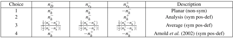
We summarise the choices in Table 1.
Choice n−D n−eh n+eh Description
1 n−h n−h −n−h Planar (non-sym)
2 n−h n−h n+h Analysis (sym pos-def)
3
1 2(n
−
h−n+h)
|1 2(n
−
h−n
+
h)|
1 2(n
−
h−n+h)
|1 2(n
−
h−n
+
h)|
1 2(n
+
h−n
−
h)
|1 2(n
+
h−n
−
h)|
Average (sym pos-def)
[image:16.612.92.502.238.305.2]4 n−h −n+h −n−h Arnoldet al.(2002) (sym pos-def)
Table 1: Choices ofn−D,n+e
handn −
eh, description of the numerical schemes they respectively lead to
and properties of resulting matrix.
We also consider the Arnoldet al.(2002) formulation with its true penalty term given by
∑
eh⊂∂Kh Z
eh
βeh(u
+
hn
+
h+u
−
hn
−
h)·(v
+
hn
+
h+v
−
hn
−
h)dsh (true penalty term).
Choosingvh=ϕ−anduh=ψ−as before yields
∑
eh⊂∂Kh Z
eh
βehψ −
ϕ−dsh.
Foruh=ψ+we now have,
∑
eh⊂∂Kh Z
eh
βehψ
+
ϕ−(n+h·n−h)dsh.
The matrices arising from Choices 2-4 are symmetric positive definite, so the Conjugate Gradient (CG) method is particularly well suited for such matrix problems. Choice 1 however yields a non-symmetric matrix, for which we use the Biconjugate Gradient Stabilized (BICGSTAB) method. All of these solvers make use of the algebraic multigrid algorithm (AMG) preconditioner coupled with the incomplete-LU factorisation preconditioner to speed up the solvers. Information on the implementation of these solvers and preconditioners in DUNE can be found in Blatt & Bastian (2007) and on their parallelisation in Blatt & Bastian (2008).
We first tested our code on a sphere where the projection algorithm described in Section 5.1 is not
required. The results showed that the expected convergence rates and the choices ofn−D,n−e
h andn
+
5.3 Test Problem on Dziuk Surface
The first test problem, taken from Dziuk (1988), considers
−∆Γu+u=f (5.4)
on the surfaceΓ ={x∈R3 : (x1−x32)2+x22+x23=1} whose exact solution is chosen to be given
byu(x) =x1x2. The outward unit normal to this surface is given byν(x) = (x1−x23,x2,x3(1−2(x1− x23)))/(1+4x23(1−x1−x22))1/2. There is no explicit projection map for mapping newly created nodes
toΓ soξ(x)has to be approximated via the ad-hoc first order algorithm described in Section 5.1.
Elements h L2-error L2-eoc DG-error DG-eoc
92 0.704521 0.243493 0.894504
368 0.353599 0.0842372 1.53 0.490805 0.87
1472 0.176993 0.0268596 1.65 0.263808 0.90
5888 0.0885231 0.00637826 2.07 0.135162 0.97
23552 0.0442651 0.00171047 1.90 0.0685366 0.98
94208 0.022133 0.000416366 2.04 0.0343677 1.00
376832 0.0110666 0.000104274 2.00 0.0171891 1.00
[image:17.612.87.497.215.325.2]1507328 0.0055333 2.60734e-05 2.00 0.0085935 1.00
Table 2: Errors and convergence orders for (5.4) on the Dziuk surface with Choice 2 (analysis).
Table 2 shows theL2andDGerrors for Choice 2. As expected, the experimental orders of
conver-gence (EOCs) match up well with the theoretical converconver-gence rates. Figure 1 shows the resulting DG approximation to (5.4) on the Dziuk surface using Choice 2.
Figure 2(a,b) shows respectively the ratios of theL2andDGerrors Erri
Err2
withi=1,3,4 where Erri
denotes the error in the corresponding norm when using Choicei. Choices 2 (analysis) and 3 (average)
appear to give the best results in both theL2andDGnorms. In particular, the additional symmetry
induced by using Choice 3 which we mentioned previously makes it the preferable choice.
A few remarks on Choice 4 with thetruepenalty term which, as mentioned before, would correspond
to the Arnoldet al.(2002) IP method onΓh: interestingly, the scheme fails to converge for such a choice.
The numerical scheme appears to be particularly sensitive to small perturbations in the off-diagonal
entries of the resulting matrix, namely the ones caused by the product of the conormalsn+h·n−h when
using the true penalty term for Choice 4. Note that in the flat case,n+h ·n−h is equal to−1. We tried
to reproduce this problem in the flat case, taking two different values for the penalty parameter oneh
depending on whether we are assembling the diagonal or the off-diagonal block. Already a factor of
10−5leads to similar problems with stability. Since Choice 4 with or without the true penalty term was
always less accurate than the other choices, we omit this choice in our next test case.
5.4 Test Problem on Enzensberger-Stern Surface
Our next test problem considers (5.4) onΓ={x∈R3 : 400(x2y2+y2z2+x2z2)−(1−x2−y2−z2)3−
40=0} whose exact solution is again chosen to be given byu(x) =x1x2. As for the previous test
problem, there is no explicit projection map so we make use of the first order ad-hoc algorithm. In this
test problem, the computation of∆Γuto derive the right-hand side of (5.4) is done via our approximation
(a)
FIG. 1: DG approximation of (5.4) on the Dziuk surface with Choice 2 (analysis).
(a) (b)
FIG. 2: Ratio of respectivelyL2andDGerrors for (5.4) on the Dziuk surface with respect to
Elements h L2-error L2-eoc DG-error DG-eoc
2358 0.163789 0.476777 0.998066
9432 0.0817973 0.175293 1.44 0.472241 1.08
37728 0.040885 0.0160606 3.45 0.150144 1.65
150912 0.0204411 0.00139698 3.52 0.0703901 1.09
603648 0.0102204 0.00033846 2.04 0.03473453 1.02
[image:19.612.86.498.99.185.2]2414592 0.00511 7.86713e-05 2.10 0.0172348 1.01
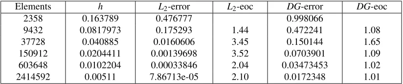
Table 3: Errors and convergence orders for (5.4) on the Enzensberger-Stern surface with Choice 2 (analysis).
Table 3 shows theL2andDGerrors for Choice 2. Although the EOCs are more erratic than for the
previous test problem, largely due to our approximation of the Laplace-Beltrami operator, they neverthe-less match up well with theoretical convergence rates. Figure 3 shows the resulting DG approximation to (5.4) on this surface using Choice 2. We again consider the DG approximation of (5.4) for different choices ofn−D,n+e
h andn −
eh. Figure 4(a,b) shows respectively the ratios of theL
2andDGerrors. These
results confirm that Choices 2 and 3 are the preferable ones to use for DG schemes on surfaces.
6. Extensions
Although our analysis was restricted to conforming grids due to the nature of the surface approxima-tion, our numerical tests suggest that the estimates of Theorem 4.1 also hold for nonconforming grids as shown in Table 4 for the Dziuk surface. Future work aims to derive a-priori error estimates for
Elements h L2-error L2-eoc DG-error DG-eoc
230 0.353599 0.21889 0.777436
920 0.176993 0.0530078 2.05 0.413817 0.91
3680 0.0885231 0.0281113 0.92 0.223119 0.89
14720 0.0442651 0.00442299 2.67 0.111518 1.00
58880 0.022133 0.00104207 2.08 0.0562128 0.99
235520 0.0110666 0.00026444 1.99 0.0281247 1.00
942080 0.00553329 6.60383e-05 2.00 0.0140544 1.00
Table 4: Errors and convergence orders for (5.4) on the Dziuk surface with Choice 2 (analysis) for a nonconforming grid.
nonconforming grids.
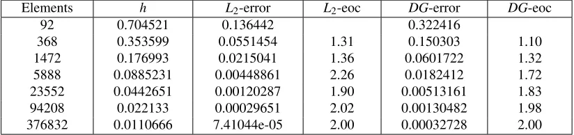
Demlow (2009) has proven that in particular, for a linear approximation of the surface and quadratic
polynomial basis functions, the FEM error scales quadratically in both theL2andH1norms. Numerical
tests suggest that our DG scheme scales similarly in the L2 andDGnorms as shown in Table 5 for
(a)
FIG. 3: DG approximation of (5.4) on the Enzensberger-Stern surface with Choice 2 (analysis).
(a) (b)
FIG. 4: Ratio of respectivelyL2andDGerrors for (5.4) on the Enzensberger-Stern surface with
Elements h L2-error L2-eoc DG-error DG-eoc
92 0.704521 0.136442 0.322416
368 0.353599 0.0551454 1.31 0.150303 1.10
1472 0.176993 0.0215041 1.36 0.0601722 1.32
5888 0.0885231 0.00448861 2.26 0.0182412 1.72
23552 0.0442651 0.00120287 1.90 0.00513161 1.83
94208 0.022133 0.00029651 2.02 0.00130482 1.98
[image:21.612.86.498.100.197.2]376832 0.0110666 7.41044e-05 2.00 0.00032728 2.00
Table 5: Errors and convergence orders for (5.4) on the Dziuk surface with Choice 3 (average) using quadratic polynomial basis functions.
Acknowledgements
This research has been supported by the British Engineering and Physical Sciences Research Council (EPSRC), Grant EP/H023364/1.
REFERENCES
AINSWORTH, M. & RANKIN, R. (2011) Constant free error bounds for nonuniform order discontinuous Galerkin finite-element approximation on locally refined meshes with hanging nodes. IMA J. Numer. Anal.,31, 254– 280.
ARNOLD, D. N. (1982) An interior penalty finite element method with discontinuous elements. SIAM J. Numer. Anal.,19, 742–760.
ARNOLD, D. N., BREZZI, F., COCKBURN, B. & MARINI, L. D. (2002) Unified analysis of discontinuous Galerkin methods for elliptic problems.SIAM J. Numer. Anal.,39, 1749–1779.
AUBIN, T. (1982) Nonlinear analysis on manifolds. Monge-Amp`ere equations. Grundlehren der Mathematischen Wissenschaften [Fundamental Principles of Mathematical Sciences], vol. 252. New York: Springer-Verlag, pp. xii+204.
BASTIAN, P., BLATT, M., DEDNER, A., ENGWER, C., KLOFKORN, R., OHLBERGER¨ , M. & SANDER, O. (2008a) A Generic Grid Interface for Parallel and Adaptive Scientific Computing. Part I: Abstract Framework. Computing,82, 103–119.
BASTIAN, P., BLATT, M., DEDNER, A., ENGWER, C., KL¨OFKORN, R., KORNHUBER, R., OHLBERGER, M. & SANDER, O. (2008b) A Generic Grid Interface for Parallel and Adaptive Scientific Computing. Part II: Implementation and Tests in DUNE.Computing,82, 121–138.
BASTIAN, P., BLATT, M., DEDNER, A., ENGWER, C., FAHLKE, J., GRASER, C., KL¨ OFKORN, R., NOLTE, M.,¨ OHLBERGER, M. & SANDER, O. (2012). http://www.dune-project.org.
BLATT, M. & BASTIAN, P. (2007) The iterative solver template library. Applied Parallel Computing. State of the Art in Scientific Computing(B. K˚agstr¨om, E. Elmroth, J. Dongarra & J. Wa´sniewski eds). Lecture Notes in Computer Science, vol. 4699. Springer, pp. 666–675.
BLATT, M. & BASTIAN, P. (2008) On the generic parallelisation of iterative solvers for the finite element method. Int. J. Comput. Sci. Engrg.,4, 56–69.
BRDAR, S., DEDNER, A. & KLOFKORN, R. (2012) Compact and stable discontinuous galerkin methods for¨ convection-diffusion problems. J. Sci. Comp.,34, 263–282.
COCKBURN, B. (2003) Discontinuous galerkin methods. ZAMM-Journal of Applied Mathematics and Mechan-ics/Zeitschrift f¨ur Angewandte Mathematik und Mechanik,83, 731–754.
DECKELNICK, K., ELLIOTT, C. & STYLES, V. (2001) Numerical diffusion-induced grain boundary motion. Interfaces Free Bound.,3, 393–414.
DEDNER, A., KLOFKORN, R., NOLTE, M. & OHLBERGER¨ , M. (2010) A Generic Interface for Parallel and Adaptive Scientific Computing: Abstraction Principles and the DUNE-FEM Module. Computing,90, 165– 196.
DEDNER, A., KLOFKORN, R., NOLTE, M. & OHLBERGER, M. (2012). http://dune.mathematik.uni-freiburg.de.¨ DEMLOW, A. (2009) Higher-order finite element methods and pointwise error estimates for elliptic problems on
surfaces. SIAM J. Numer. Anal,47, 805–827.
DEMLOW, A. & DZIUK, G. (2008) An adaptive finite element method for the laplace-beltrami operator on implic-itly defined surfaces.SIAM Journal on Numerical Analysis,45, 421–442.
DZIUK, G. (1988) Finite elements for the Beltrami operator on arbitrary surfaces. Partial differential equations and calculus of variations. Lecture Notes in Math., vol. 1357. Berlin: Springer, pp. 142–155.
DZIUK, G. & ELLIOTT, C. (2007a) Surface finite elements for parabolic equations.J. Comput. Math,25, 385–407. DZIUK, G. & ELLIOTT, C. M. (2007b) Finite elements on evolving surfaces. IMA J. Numer. Anal.,27, 262–292. ELLIOTT, C. & STINNER, B. (2010) Modeling and computation of two phase geometric biomembranes using
surface finite elements. J. Comp. Phys.,229, 6585–6612.
GIESSELMANN, J. & M ¨ULLER, T. (2013) Geometric error of finite volume schemes for conservation laws on evolving surfaces.submitted to Numerische Mathematik.
JAMES, A. & LOWENGRUB, J. (2004) A surfactant-conserving volume-of-fluid method for interfacial flows with insoluble surfactant.J. Comp. Phys.,201, 685–722.
JU, L. & DU, Q. (2009) A finite volume method on general surfaces and its error estimates.Journal of Mathemat-ical Analysis and Applications,352, 645–668.
NEILSON, M. P., MACKENZIE, J. A., WEBB, S. D. & INSALL, R. H. (2011) Modeling cell movement and chemotaxis using pseudopod-based feedback.SIAM J. Sci. Comput.,33, 1035–1057.
RINEAU, L. & YVINEC, M. (2009) 3d surface mesh generation. CGAL Editorial Board, editor, CGAL User and Reference Manual,3, 53.