On sample selection models and skew distributions

(1)

University of Warwick institutional repository: http://go.warwick.ac.uk/wrap

A Thesis Submitted for the Degree of PhD at the University of Warwick

http://go.warwick.ac.uk/wrap/57678

This thesis is made available online and is protected by original copyright.

Please scroll down to view the document itself.

(2)

AUTHOR:Emmanuel Olusegun Ogundimu DEGREE:Ph.D.

TITLE:On Sample Selection Models and Skew Distributions

DATE OF DEPOSIT: . . . .

I agree that this thesis shall be available in accordance with the regulations governing the University of Warwick theses.

I agree that the summary of this thesis may be submitted for publication. I agree that the thesis may be photocopied (single copies for study purposes only).

Theses with no restriction on photocopying will also be made available to the British Library for microfilming. The British Library may supply copies to individuals or libraries. subject to a statement from them that the copy is supplied for non-publishing purposes. All copies supplied by the British Library will carry the following statement:

“Attention is drawn to the fact that the copyright of this thesis rests with its author. This copy of the thesis has been supplied on the condition that anyone who consults it is understood to recognise that its copyright rests with its author and that no quotation from the thesis and no information derived from it may be published without the author’s written consent.”

AUTHOR’S SIGNATURE: . . . .

USER’S DECLARATION

1. I undertake not to quote or make use of any information from this thesis without making acknowledgement to the author.

2. I further undertake to allow no-one else to use this thesis while it is in my care.

DATE SIGNATURE ADDRESS

. . . .

(3)

On Sample Selection Models and Skew

Distributions

by

Emmanuel Olusegun Ogundimu

Thesis

Submitted to the University of Warwick

for the degree of

Doctor of Philosophy

Department of Statistics

(4)

List of Tables

2.1 Missingness per question during the trial; 599 patients. . . 22 2.2 Scoring Interval and Overall missingness with Measurement time. . . 22

3.1 Simulation results (multiplied by 10,000) using skew-distributions to model selectively reported data. Selection and Outcome equations

have the same covariates. . . 40

3.2 Simulation results (multiplied by 10,000) using skew-distributions to model selectively reported data. Selection equation has one more

covariate that is not in Outcome equation. . . 40

3.3 Fit of Azzalini (1985) model, ESN and EGSN model to complete case NDI scores at 8 months. λ1 andλ2 are constrained to be equal in the

EGSN model. . . 41

3.4 Fit of truncated normal (TN) and truncated skew-normal (TSN) models to complete case NDI scores at 8 months. . . 43

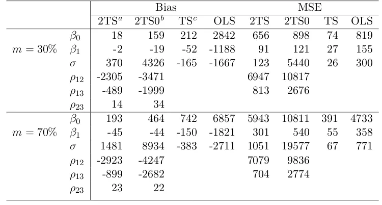
4.1 Simulation results (multiplied by 10,000) in the presence of exclusion

restriction. . . 55 4.2 Simulation results (multiplied by 10,000) in the absence of exclusion

restriction. . . 56

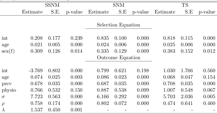
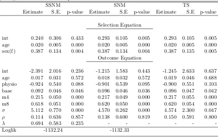
4.3 Probit model for dropout at 4, 8 and 12 months using Vernon scores. 57 4.4 Fit of selection skew-normal model (SSNM), Selection-normal model

(SNM), and Heckman two-step model to the NDI scores at 8 months. 58 4.5 Fit of selection skew-normal model (SSNM) with 6 fixed value of ρ

to the NDI scores at 8 months. . . 62

4.6 Fit of selection skew-normal model (SSNM), Selection-normal model (SNM), and Heckman two-step model to the NDI scores at 12 months. 63

(9)

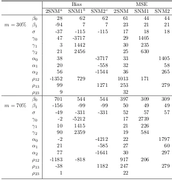
5.1 Simulation results (multiplied by 10,000) for the likelihood based

es-timator of two-level selection model. . . 82 5.2 Simulation results (multiplied by 10,000) for the moment based

esti-mator of two-level selection model. . . 83

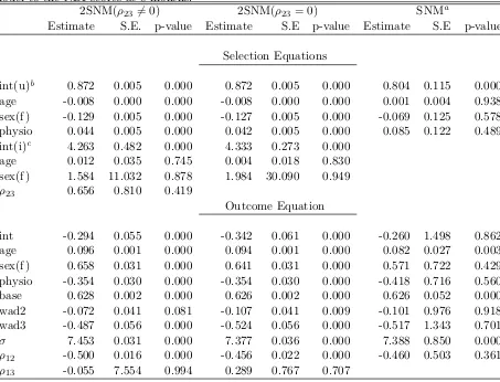
5.3 Probit model for dropout at months 8. . . 84 5.4 Fit of Two-level selection models (ρ236= 0) &ρ23= 0), and Heckman

selection model to the NDI scores at 8 months. . . 85

6.1 Fit of SHASH model, SN model, and classical Heckman model (SNM) to a sample selection dataset with bivariate normal error distribution. 103

6.2 Simulation results (multiplied by 10,000) in the presence of exclusion

restriction. . . 105 6.3 Simulation results (multiplied by 10,000) in the absence of exclusion

restriction. . . 106

6.4 Empirical significance levels (as %) of the tests of symmetry for the nominal significance levelα = 0.05 in the SHASH model. . . 108

6.5 Powers (as %) of the tests of symmetry for the nominal significance levelα = 0.05 in the SHASH model. . . 108

6.6 Fit of copula-based Sinh-archsinh (SHASH), Skew-normal (SN), and

Selection-normal model (SNM) sample selection models to the NDI scores at 8 months. The corresponding outcome models are truncated

at [0,50]. . . 109

6.7 Fit of copula-based Sinh-archsinh (SHASH), Skew-normal (SN), and Selection-normal model (SNM) sample selection models to the NDI

scores at 8 months. The corresponding outcome models are

untrun-cated. . . 110

7.1 Distribution of the Number of Recurrences observed for the patients

the three treatment groups in bladder cancer trial. . . 116

7.2 Summary statistics for the follow-up times of patients in the three treatment groups in bladder cancer trial. . . 116

7.3 Bias and MSE in estimated treatment effect with 30% missing data

in both placebo and treated arm: Asymptotic and Bootstrap impu-tations. Simulation results (multiplied by 10,000). . . 131

7.4 Bias and MSE in estimated treatment effect with 30% and 40%

(10)

7.5 Bias and MSE in estimated treatment effect with 30% missingness in

both placebo and treated arm: Uniform and Normal random effects. Simulation results (multiplied by 10,000). . . 133

7.6 Proportion of events observed in treatment group using simulated

data for the models,n=1000, 1000 replications and censoring at 112 days. . . 136

7.7 Bias and MSE in estimated treatment effect under the Weibull,

Con-ditional, Poisson and Autoregressive data generation process. Im-putation was done under mixed Poisson process. Simulation results

(multiplied by 10,000). . . 137

7.8 Imputation of treated arm using placebo rate λp(t). A and P stand

for active and placebo arms respectively. . . 139

7.9 Fit of Direct Likelihood, Asymptotic Imputation and Bootstrap

Im-putation to the bladder cancer data. . . 140 7.10 Fit of Asymptotic Imputation and Bootstrap Imputation to the

blad-der cancer data using event rates in the placebo arm to impute data

in the treated arm. . . 140 7.11 Fit of Bootstrap Imputation to the bladder cancer data using higher

rate than the MAR rate. Bold face entries are significant at 5% level of significance. . . 141

A.1 Simulation results (multiplied by 10,000) for λ= 1 and varyingρ in

the presence of exclusion restriction. . . 151 A.2 Simulation results (multiplied by 10,000) for λ= 2 and varyingρ in

the presence of exclusion restriction. . . 152

A.3 Imputation with new rate λ_new,trt(t). 30% data is missing in both the treated and the placebo arm. . . 155

A.4 Imputation with new rateλ_new,trt(t), 10% and 30% data is missing

in placebo and treated arm respectively. . . 156 A.5 Imputation with new rateλ_new,trt(t), 10% and 40% data is missing

(11)

List of Figures

2.1 Comparison of Skew-normal densities . . . 10

2.2 Contour plot and 3-d plot of a bivariate SN2(µ,Ω,λ) with µ = (−0.1,0.1), Ω = diag(1,1) and λ= (−1,1) . . . 12

2.3 Marginal distributions and Correlations at Baseline, Month 4, 8 and 12 for the NDI scores . . . 24

2.4 Chi-square plots for items at baseline, month 4, month 8 and month 12 24 2.5 Q-Q plots for residuals of scores at baseline, month 4, month 8 and month 12 . . . 24

3.1 Two indistinguishable parameter combination for two-parameter ESN, ∆((3,2),(2,1.3)) = 0.01 . . . 32

3.2 Comparison of generalized skew-normal densities . . . 35

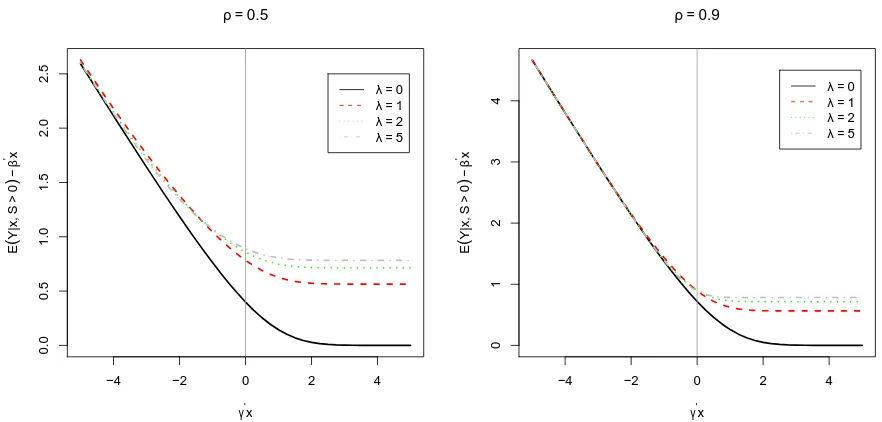
4.1 Plot of correction factor for different values of skewness parameter withλ= 0 corresponding to the normal case. . . 51

4.2 Plot of correction factor for different values of skewness parameter withλ= 0 corresponding to the normal case. . . 51

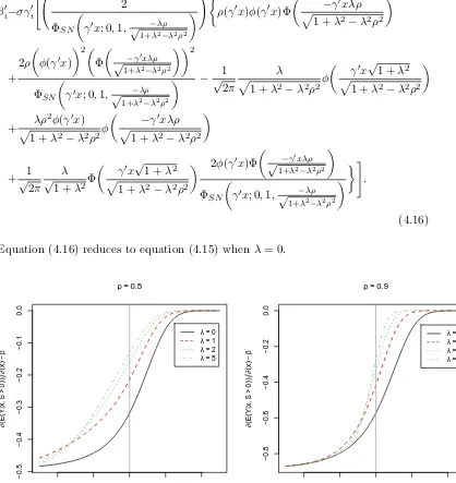
4.3 Plot of marginal effect for different values of skewness parameter with λ= 0 corresponding to the normal case. . . 52

4.4 Plot of marginal effect for different values of skewness parameter with λ= 0 corresponding to the normal case. . . 52

4.5 Fitted SSNM model. . . 59

4.6 Fitted SNM model. . . 59

4.7 Fitted Two-step model. . . 59

4.8 Profile log-likelihood forλfor the NDI scores (SSNM model). . . 60

(12)

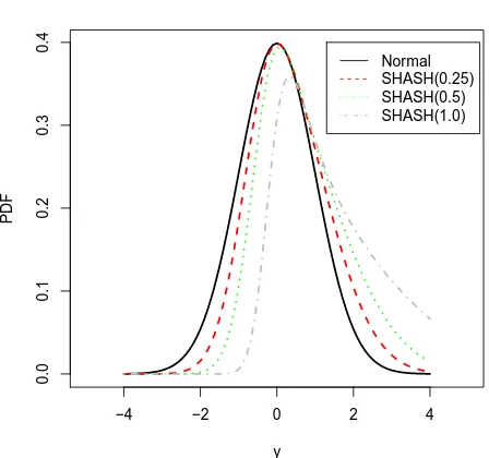
6.1 Comparison of SHASH densities. . . 100

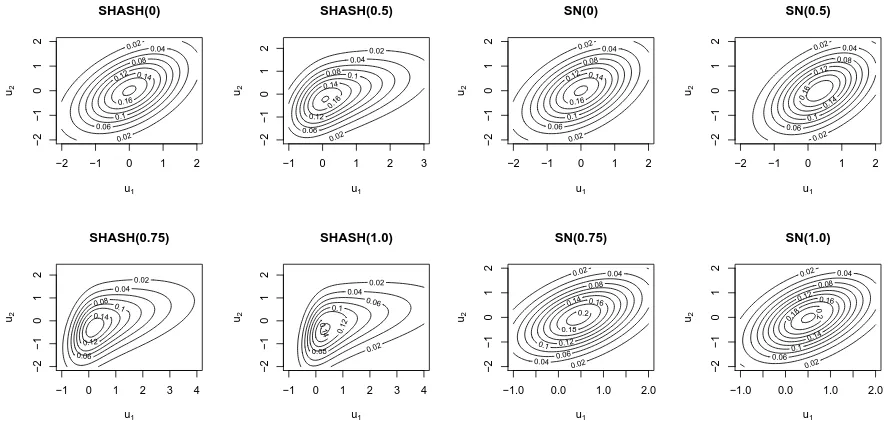
6.2 Contour plots of SHASH distribution with ρ= 0.5 between marginals. 101 6.3 Contour plots of SN distribution withρ= 0.5 between marginals. . . 101

6.4 Q-Q plots of SHASH( = 1.0) and SN(λ = 1.0) margins from a

bivariate Gaussian copula with correlation 0.5 and normal margins. . 102 6.5 Profile likelihood for using SHASH model. Data generated from a

bivariate normal distribution with ρ= 0.5. . . 104

6.6 Profile likelihood for λ using SN model. Data generated from a bi-variate normal distribution withρ= 0.5. . . 104

6.7 Profile likelihood forρusing SHASH and SN model. Data generated

from a bivariate normal distribution withρ= 0.5. . . 107 6.8 Profile likelihood forσ using SHASH and SN model. Data generated

(13)

Acknowledgments

Let me begin by expressing my deepest gratitude to my supervisor, Prof. Jane

Luise Hutton for her support and encouragement which enabled me to complete

this thesis. She believes in me as a mother would do with her child. Thanks

for introducing me to skew distributions and pointing me in the right direction to

better my future career in statistics. The technical support, and time given to me

during the preparation of the thesis is invaluable. The four Xmas celebrated during

the period of my studentship were celebrated home away from home at her place.

Thanks for the tasty dishes. May you live long to eat the fruits of your labor. I

sincerely look forward to future collaboration with you because no one ever forgets

a good teacher. Thank you again and again!

I am very grateful to my examiners, Dr. Ewart Shaw and Prof. David Firth.

The feedback from Dr. Shaw on my second year report improved the final draft of

this thesis. Prof. Firth’s critical view on ceiling and floor effects of bounded scores

on likelihood-based inference motivated the use of truncated distributions in the

thesis. A big thank you to Prof John Copas for helpful insight that improved this

work. I wish him all the very best in his retirement. Thanks to Prof. Sallie Lamb

and the MINT trial team for the permission to use the Neck disability index data.

My PhD research was funded by the Engineering and Physical Sciences Research

Council grant, for the Centre for Research in Statistical Methodology. I am grateful

to the Department of Statistics for this grant.

I received a very warm reception and hospitality during my three months

placement at Novartis Pharma, Switzerland. Many thanks to Mouna Akacha for all

(14)

Frank Bretz for the opportunity to be part of ‘the Novartis dream’. May God bless

you.

Many people contributed to my academic career till date. I thank all my

teachers. In particular, Prof. Geert Molenberghs who has been of tremendous

assistance. He is ever ready to give me his shoulder to stand on and see farther. I

appreciate my Professor and mentor, Prof. Adewale R. Solarin for his support. I

appreciate my former Heads of Department, Prof. Kaku Sagary Nokoe and Prof.

James Adedayo Oguntuase for their support and love. May the Lord reward you.

My appreciation is definitely incomplete without mentioning friends and

fam-ily. I appreciate my Mum that taught me that hard work and perseverance pay. She

is fond of our local version of the French proverb, ‘One may go a long way after one

is tired’. Out of sight is indeed not always out of mind. A big thanks to my uncle,

Johnson Sunday Olawunmi, for his incessant calls to check how I am fairing during

the last three and a half years. It is of course true that behind every successful man,

there is a woman. Thanks to my angel Oluwakemi Racheal Adeboye for her patience

and unalloyed support throughout the period of my PhD research. You are an angel

indeed! Dr. Peter Kimani was my first Warwick friend and he has been of enormous

support. I am very grateful Peter, God bless you. I had interesting discussions with

my colleague, Javier Rubio on skew distributions. Thank you Javier. Alex Thiery

was and is still a good friend and colleague. God bless you.

Above all, I appreciate God who was my help in ages past, my hope for years

(15)

Declarations

I declare that the work in this thesis is my own, and has not been submitted

else-where for examination. The materials that are not my original ideas have been

acknowledged by referencing. The work in Chapter 7 was done jointly with Mouna

(16)

Abstract

This thesis is concerned with methods for dealing with missing data in non-random samples and recurrent events data.

The first part of this thesis is motivated by scores arising from questionnaires which often follow asymmetric distributions, on a fixed range. This can be due to scores clustering at one end of the scale or selective reporting. Sometimes, the scores are further subjected to sample selection resulting in partial observability. Thus, methods based on complete cases for skew data are inadequate for the analysis of such data and a general sample selection model is required. Heckman proposed a full maximum likelihood estimation method under the normality assumption for sample selection problems, and parametric and non-parametric extensions have been proposed.

A general selection distribution for a vectorY∈_Rp _{has a PDF}_f

Y given by

fY(y) =fY?(y)

P(S?∈C|Y? =y)

P(S?_∈_C₎ ,

whereS?∈_Rq_and_Y? _∈

Rpare two random vectors, andCis a measurable subset of Rq. We use this generalization to develop a sample selection model with underlying

(17)

The second part of this thesis is motivated by studies that seek to analyze processes that generate events repeatedly over time. We consider the number of events per subject within a specified study period as the primary outcome of interest. One considerable challenge in the analysis of this type of data is the large proportion of patients that might discontinue before the end of the study, leading to partially observed data. Sophisticated sensitivity analyses tools are therefore necessary for the analysis of such data.

(18)

Abbreviations

base Baseline measurement for the NDI scores

CDF Cumulative Distribution Function

CSN Closed Skew-Normal

DL Direct Likelihood

EGSN Extended (two-parameter) Generalized Skew-Normal

ESN Extended Skew-Normal

int Intercept

l0HR l0Hospital’s Rule

Loglik Log-likelihood value

LRT Likelihood Ratio Test

MAR Missing At Random

MCAR Missing Completely At Random

mgf Moment Generating Function

MI Multiple Imputation

MLEs Maximum Likelihood Estimates

MNAR Missing Not At Random

MSN Multivariate Skew-Normal (Azzalini’s Skew-normal distribution)

NDI Neck Disability Index

Num Number of tumor (Bladder cancer data)

PDF Probability Density Function

Physio Physiotherapy treatment

pMI Placebo Multiple Imputation

(19)

Q-Q plot Quantile-Quantile plot

S.E Standard Error

SHASH Asymmetric subfamily of Sinh-Arcsinh distribution

Size Size of tumor (Bladder cancer data)

SN Skew-Normal (Azzalini’s univariate Skew-normal distribution)

SNM Selection Normal Model

SSNM Selection Skew-Normal Model

SUN Unified Skew-Normal

SUT Unified Skew-t

TS Heckman Two-step Method

TSN Truncated Skew-Normal

(20)

Chapter 1

Introduction

This thesis discusses issues arising with missing data, in two parts. The first part is devoted to the unification of missing data problems into a distributional framework,

while the second part considers a distinct, but related, concept of dealing with

missing data in a recurrent events data framework.

The first part of the thesis is motivated by a study where pain related

ac-tivity restriction is measured repeatedly over time using the neck disability index

(NDI) questionnaire (Vernon and Mior, 1991). In this type of study, the patient’s perception of his or her well-being is usually the most important outcome of

inter-est. These are broadly termed quality of life (QoL) outcomes. Scores arising from

instruments designed to assess QoL (e.g. screening questionnaires) often follow asymmetric distributions due to skewness inherent in Likert-scale type instruments.

Indeed, skewness related studies are not uncommon in psychology literature. In

addition, the realized samples from the underlying discrete process are further sub-jected to selective reporting and missing data, with the scores reflecting a selected

population. Consequently, there is need for a general model for sample selection

with inherent skewness.

The two most common deviations from normality are heavier tails and

skew-ness. In dealing with heavier tails in sample selection, Marchenko and Genton

(2012) derived a model using links between hidden truncation and sample selection but with an underlying bivariate-t error distribution. They noted that a more

ap-pealing flexible parametric model is needed to be considered that can accommodate

heavy tails and skewness. A skew-normal distribution (Azzalini, 1985) could be a good candidate to accommodate skewness.

(21)

effects at a measurement occasion may be desirable and a cross-sectional view of

the data will make two missing data type inevitable- unit and item non-response. Unit non-response occurs when the whole questionnaire is missing for a patient and

item non-response occurs where a response has not been provided for a question.

The traditional practice is to use weighting adjustment for unit non-response and imputation methods for item non-response. Weighting adjustment means weights

are assigned to sample respondents in order to compensate for their systematic

differences relative to non-respondents, whereas imputation involves filling in missing values (singly or multiply) to produce complete data set.

Although these methods have reached a high level of sophistication, they

normally assume that the missing data mechanism is missing at random (MAR), an assumption that cannot be verified using the observed data alone. Apart from this,

patients may refuse to answer sensitive questions (e.g. underlying health issues or

drug addiction) on a questionnaire for reasons related to the underlying true values for those questions. In multivariate settings with arbitrary patterns of non-response,

imputation, and hence the MAR assumption, is convenient computationally, but it

is often implausible (Robins and Gill, 1997). In this setting, MAR means that a patient’s probabilities of responding to items may depend only on his or her own

set of observed items, which is an unrealistic assumption. Specifically, the use of mean imputation is justifiable if items within the scale are strongly correlated

with each other but correlation with external factors is low relative to within-scale

correlations. This cannot be readily established in practice. Thus, when we suspect that non-response may depend on missing values, then a proper analysis will be to

model jointly the population of complete data and the non-response process. Sample

selection models are therefore viable tool.

A selection model was introduced by Heckman (1976). He proposed a full

maximum likelihood estimation under the assumption of normality. His method

was criticized on the ground of its sensitivity to normality assumption prompting him to develop the two-step estimator (Heckman, 1979). Sample selection models,

also referred to as models with incidental (hidden) truncation, arise in practice as

a result of the partial observability of the outcome of interest in a study. The data are missing not at random (MNAR) because the observed data do not represent a

random sample from the population, even after controlling for covariates. Although

the model has its origin from the field of Economics, it has been applied extensively in other social sciences, and in medicine. A prominent application to treatment

allocation for patients and links with the skew-normal distribution was discussed by

(22)

There are situations where a variable is skewed and yet the residuals are

approximately normal when the skewed variable is conditioned on other variables. This however, is not the case with bounded scores since the data exhibits ceiling and

floor effects and the skewness could be natural consequences of this. The classical

approach is to transform the data to near normality so that a linear regression model can be used. This may not remove the non-linear dependence of the transformed

scores on covariates because of the bounds (see Hutton and Stanghellini (2011)). In

fact, if such transformations exist, they are not always appropriate in modeling data resulting from selectively reported samples because interest is in making inference

in the unselected population. There is additional disadvantage of not working on

the original scale familiar to the health care professionals.

In view of these limitations, we propose extensions of Heckman (1976) and

Heckman (1979) models by adding two additional features in a parametric

frame-work. First, a skew-normal error distribution is used as an underlying error dis-tribution. This model allows us to establish a link between the continuous

compo-nent of our model log-likelihood function and an extended version of a generalized

skew-normal distribution (Jamalizadeh et al., 2008). Sensitivity analysis for the as-sumption of selection is readily carried out using the profile likelihood in a manner

similar to the Copas and Li (1997) approach. In addition, the link is used to derive the expected value of the model, which extends Heckmans two-step method.

Sec-ondly, sample selection model is unified into a distributional framework. This allows

for straightforward extensions of Heckman’s models into multilevel and longitudinal framework. In particular, the model is used to analyze jointly a data set with unit

and item non-response. Sample selection models using Gaussian copula are also

investigated.

The second part of this thesis is motivated by a study that compares an

active treatment with a placebo in a recurrent event data framework, subject to

informative dropout. The aim is to provide a tool for sensitivity analysis in such studies. Recurrent event data arise in practice when a subject experiences the

same type of event repeatedly over time. Unlike in a classical survival study where

patients can experience at most a single event, patients can experience multiple events in recurrent event data framework. For example, in clinical research, repeated

seizures in epileptic patients, flares in gout studies or repeated asthma attacks can

be classified as recurrent events.

A point process formulation is commonly used to describe and analyse

recur-rent event data and the two most commonly used approaches are the event counts

(23)

based on event counts are used to describe situations where events occur randomly

in such a way that the numbers of events in non-overlapping time intervals are statis-tically independent. These models are often used for frequently occurring events in

a subject. On the other hand, the gap time approaches are often used when events

are relatively infrequent. This method is ideal for situations where prediction of time to next event is of interest, and is very common in studies that investigate

system failures. Our focus in this part of the thesis will be on event counts and the

traditional framework for its analysis, the Poisson process.

Recurrent event data analysis takes the whole evolution of the recurrent

events into account. There are potential problems in the presence of dropout. First,

if we assume an intention to treat analysis (ITT, i.e. patients data are analyzed in the treatments groups they are randomized to and not on the treatments they eventually received)we need to take into account the follow-up time. This is because the number of events may be the same for two patients but the number of counts per unit time, (i.e. number of count/follow-up time) may differ substantially. For

example, a patient who drops out, say, after the second event, due to toxicity has

event count of two. On the other hand, there might be less dropout in the placebo group with high number of events. Thus, the treatment might appear to be effective

when in fact the latent reason is the high dropout rate in the treated group. Of course, the dropout time can be adjusted for in the model and this will give valid

analysis if the missingness process is unrelated with the outcome process. This does

not give sufficient flexibility to examine other types of missing data mechanism that can also bias the treatment comparison.

Consequently, we examine in a simulation study how data analyses results

can depend on assumptions of MAR and MNAR, and the imputation methods used to impute the missing data. The flexibility and transparency of multiple imputation

makes it attractive for this work. In addition, multiple imputation separates the

solution of the missing data problem from the solution of the complete data problem. The missing data problem is first solved before solving the complete data problem.

The fact that these two phases can be separated gives a better insight into the

scientific problems we study in this part of the thesis. We also investigate the importance of varying event generation process (see (Metcalfe and Thompson, 2006;

(24)

1.1 Overview of Thesis

The thesis has eight chapters and is organized in two parts. The first part is

mo-tivated by the MINT trial (Managing Injuries of the Neck Trial) which uses the NDI scores, and the second is motivated by a publicly available bladder cancer data

set. In the introductory part, we pointed out that selectively reported outcomes

often leads to skewness. This selectivity may result not only from decisions on sampling design but also from self-selection. An overview of relevant literature on

skew-normal distribution is provided in chapter 2. Given that the univariate and

multivariate normal distributions are well known, we will assume that the underly-ing process follows normal laws. Since selection under the normal process leads to

the familiar Azzalini (1985) (or its extension) skew-normal distribution, this allows us to describe their connections with missing data. Exploratory analysis of the data

set used in this part of the thesis and the concept of missing data concludes this

chapter.

Methods that ignore the missing data process are discussed in chapter 3. In

particular, we introduce a new class of skew-normal distribution which we referred to

as anextended two-parameter generalized skew-normal distribution. The implication of using skew-normal distributions to model data arising from sample selection is

evaluated in a simulation study, and data example concludes this chapter.

In chapter 4, we develop a sample selection model with underlying skew-normal distribution which we referred to as selection skew-skew-normal model (SSNM).

Its moment estimator was derived using the link between skew models arising from

selection and hidden truncation formulation of skew models. The moment esti-mator is shown to extend Heckman two-step method. A simulation study is used

to demonstrate the superiority of the SSNM model over the conventional sample

selection model and data application is considered. We conclude this chapter by proposing a multivariate extension of this model in a straightforward way.

In chapter 5, we propose a unified approach for multilevel sample selection

models in a parametric framework by treating the outcome variable as the non-truncated marginal of a non-truncated multivariate normal distribution. The resulting

density for the outcome is the continuous component of the sample selection

den-sity, and has links with the closed skew-normal distribution. The closed skew-normal distribution provides a framework which simplifies the derivation of the conditional

expectation and variance of the observed data. We use this to generalize the Heck-man’s two-step method to a multilevel sample selection model. This model is used

(25)

A major draw-back of the model proposed in chapter 4 is that a solution

to the score equations always exists associated with the skewness parameter equals to zero. This feature is inherited from the underlying Azzalini (1985) skew-normal

distribution used. To circumvent this problem, we propose in chapter 6, the use of

Gaussian copula in a sample selection framework with the Jones and Pewsey (2009) sinh-arcsinh distribution as marginals. We examine the power of Wald test and LRT

for the hypothesis of symmetry. We conclude the chapter with the examination of

the impact of boundedness in the NDI scores on inherent skewness in the data using sample selection models with truncated marginal distributions for the outcomes.

The second part of this thesis focus on imputation of missing data in

recur-rent event data study. We propose a method for artificially creating the missing recurrent event sequence for the data under the assumption that patients get no

benefit if they stop taking the active treatment. This method of imputation is

re-ferred to as placebo multiple imputation (pMI). The MAR assumption implies that the future statistical behavior of the observations from a subject, conditional on the

history, is the same whether the subject drops out (deviates) or not in the future.

Based on this, we propose sensitivity analysis tools in a simulation study by imput-ing missimput-ing data for patients in the active treatment with higher event rate than

the one determined by the MAR assumption. In chapter 7, we review models for recurrent event data, and two frequentist based imputation methods are evaluated.

To make the method readily available to applied statisticians, we give an easy to

follow algorithm to execute the imputation model. A scenario evaluation study to compare the performances of the methods proposed in this part is also studied. A

data example completes this chapter.

(26)

Part I

On Sample Selection Models

(27)

Chapter 2

Literature Review

There is an enormous body of literature that address skew distributions and sample selection separately and jointly. Arguably, most of the works are very general and

well grounded mathematically. However, these works have been applied sparingly

in modeling real life data. We present the Azzalini (1985) skew-normal distribution and its links with sample selection problems. Other methods for the construction of

skew distributions are discussed. In addition, we introduce the data set that is used

in this part of the thesis. Data exploration which motivated the models proposed in the thesis is also evaluated. Concepts of missing data conclude this chapter.

2.1 Skew-Normal Distribution

The skew-normal distributions are extensions of the normal distribution which ad-mit skewness whilst retaining most of the interesting properties of the normal

dis-tribution. Their popularity, since the Azzalini (1985) paper, has led to intense development of this class. The developments are so numerous that it is confusing to

applied statisticians which class of skew-normal model is most appropriate for data

analysis. The relationship between these models are discussed below.

2.1.1 Univariate Skew-normal distribution

A random variable (r.v)Z is said to have a skew symmetric distribution generated

byg and π, if its probability density function (PDF) is

(28)

where g is a PDF symmetric about 0 and π is a Lebesgue measurable function

satisfying 0 ≤ π(z) ≤ 1 and π(z) +π(−z) = 1, almost everywhere on R. The

functionπ is called a skewing function.

Skew-symmetric distributions have been investigated by many authors. For

variousπ, Nadarajah and Kotz (2003) and Arellano-Valle et al. (2004) studied the properties of skew-symmetric distributions withg=φ, the standard normal density.

The cases in which π(z) ≡Ψ(λz), λ, z∈ _R where Ψ is a CDF with Ψ0 symmetric about 0, andg is any of the following PDFs: normal, Student’s t, Cauchy, Laplace, logistic, and uniform has also been investigated (see Gupta et al. (2002)).

The theory of skew-symmetric distributions begins with the Azzalini (1985)

paper where g(z) = φ(z) is combined with the skewing function π(z) = Φ(λz), where Φ denotes the standard normal CDF.

Definition 1. Let Z be a continuous random variable. Let φ and Φ denote the standard normal density and corresponding distribution function respectively. Then

Z is said to have a skew-normal distribution with parameterλ∈R if the density of

Z is

f(z;λ) = 2φ(z)Φ(λz), z∈_R (2.2)

and we writeZ ∼ SN(λ).

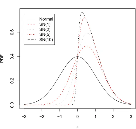
The componentλis called the shape parameter because it regulates the shape of the density function. Whenλ= 0, the density is the standard normal. Figure 2.1

shows the densities corresponding to 4 different positive skewness. It can be seen

that the model converges to half-normal distribution very fast asλincreases, even for values ofλ as small as 5 or 10. In practice, to fit data, we work with an affine

transformationY =µ+σZ ,µ∈_Rand σ >0. The density ofY is then written as

f(y;µ, σ, λ) = 2

σφ

y−µ

σ

Φλy−µ σ

, (2.3)

and we writeY ∼SN(µ, σ, λ). A convolution type stochastic representation of (2.2) in terms of a normal and a half normal was given by Henze (1986). IfY0 andY1 are

independentN(0,1) random variables and δ∈[−1,1], then

Z =δ|Y0|+

p

1−δ2_Y 1,

isSN(λ), where λ=δ/√1−δ2_.

(29)

−3 −2 −1 0 1 2 3

0.0

0.2

0.4

0.6

Different PDFs of Skew−normal Distributions

z

PDF

[image:29.595.181.443.132.380.2]

Normal SN(1) SN(2) SN(5) SN(10)

Figure 2.1: Comparison of Skew-normal densities

• E(Z) =λp2/π

• Var(Y)= 1−_πλ22

• Skewness indexγ =

2/π 3/2

2−π/2

sign(λ)λ2 .

1−2λ2/π 3/2

∈[-0.995,0.995].

The CDF of (2.2) is

2

Z z

−∞

Z λs

−∞

φ(s)φ(t)dtds= 2Φ2

z,0;−λ.p1 +λ2_,

where Φ2 is the CDF of a standard bivariate normal distribution.

The skew-normal distribution and its multivariate counterparts suffer from

two inferential drawbacks. When the skewness parameter equals zero, the profile

likelihood for skewness admits stationary points for any sample of any size, and the Fisher information matrix is singular. These problems have not limited the

usefulness of the distribution in practice (see Pewsey (2000), Ley and Paindaveine

(30)

2.1.2 Multivariate Skew-normal distribution (MSN)

The multivariate skew-normal distribution, like its univariate counterpart, has some

properties similar to the normal distribution and includes the normal distribution

as a special case.

Definition 2. A random vector Z=(Z1, . . . , Zp)0 is a p-dimensional skew-normal,

denotedZ ∼SNp( ¯Ω,λ), if it is continuous with PDF

f(z) = 2φp(z; ¯Ω)Φ(λ0z), z∈Rp (2.4)

where φp(z; ¯Ω) denotes the PDF of the p-dimensional multivariate normal

distribu-tion with standardized marginals and correladistribu-tion matrixΩ¯.

Ifp= 2, the PDF given in (2.4) becomes

f(z1, z2) = 2φ2(z1, z2;ω)Φ(λ1z1+λ2z2), (2.5)

whereωis the off-diagonal element of ¯Ω. As in the univariate case, when a

location-scale transformation of the type Y = µ+SZ is applied, we have the PDF of Y

as

f(y) = 2φp(y;µ,Ω)Φ(λ0S−1(y−µ)),

where Ω = SΩ¯S, and we write Y ∼ SNp(µ,Ω,λ), where µ = (µ1, . . . , µp)0, S =

diag(σ1, . . . , σp). Like the univariateSN, density 2.4 has some attractive properties:

• Ifλ=0, then the model reduces to standard multivariate normal.

• If Y ∼ Np(0,Ω) and¯ Z ∼ SNp( ¯Ω,λ), then Y0Ω¯−1Y and Z0Ω¯−1Z have the

same distribution i.e. χ2_p

• IfZ∼SNp( ¯Ω,λ) andB is a symmetric positive semi-definite p×pmatrix of

rankk such thatBΩ¯B =B, then Z0BZ∼χ2_k.

Details on how to generateM SN distribution including multivariate generalization

of Henze (1986) can be found in Genton (2004).

The contours of the bivariate skew-normal density are not elliptical (see

Fig-ure 2.2). This implies that the correlation coefficient is not a good measFig-ure of

association between the two bivariate variables. The implication of this will be discussed in chapter 4. Although the distributions have properties similar to the

normal distribution, they lack the important property of closure under conditioning

(31)

Theorem 1. Let (Z1, Z2)0 ∼SN2. The conditional density f(Z2|Z1=z1) is

φc(z2|z1;ω)Φ(λ1z1+λ2z2)

Φ(λ1z1)

, (2.6)

whereφc(z2|z1;ω) denotes the conditional density associated with a bivariate normal variable with standardized marginals and correlationω.

Equation (2.6) belongs to the extended skew-normal (ESN) family (Azzalini and Dalla Valle, 1996; Capitanio et al., 2003).

x

y z

Bivariate Skew−normal Plot Bivariate Skew−normal Contours

x

y

0.02

0.04

0.06

0.08

0.1

0.12

0.14 0.16

0.18

0.2

−2 −1 0 1 2

−2

−1

0

1

2

Figure 2.2: Contour plot and 3-d plot of a bivariate SN2(µ,Ω,λ) with µ =

(−0.1,0.1), Ω = diag(1,1) and λ= (−1,1)

2.1.3 Extended Skew-normal distribution (ESN)

Since theM SN distribution lacks the closure property under conditioning, a slight

extension of this class to the so-called extended skew-normal distribution (ESN) is necessary. The ESN distribution permits the construction of multivariate skewed

models that have marginal and conditional densities that are of the same form.

However, the cost to be paid for gaining the latter is the loss of theχ2 distribution of certain quadratic form (Capitanio et al., 2003). We present here the definition

of the multivariate ESN distribution and from it derive the univariate equivalence. Identifiability issues of the distribution are discussed in chapter 3, and the model

forms the background of what is to be used in chapter 4.

(32)

distri-bution, denoted by Z∼ ESNp( ¯Ω,λ0,λ), if it is continuous with PDF

f(z) = φp(z; ¯Ω)Φ(λ0+λ 0_z₎

Φ(τ) , z∈R

p_,

where λ0=τ/

√

1−δ0_Ω¯−1_δ_, _λ_{= ¯}_Ω−1_δ_/√₁₋_δ0_Ω¯−1_δ_{, and}_δ_{= ¯}_Ω−1_λ_/√_{1 +}_λ0_Ωλ¯ _. Here, λ0 and λ are the p-dimensional vector of shift and scale parameters

respectively. For data analysis purpose, if we introduce a location-scale

transforma-tion,Y=µ+ωZ, whereµand ω are as defined in section 2.1.2, then

f(y) = φp(y;µ,Ω)Φ(λ¯ 0+λ

0_ω−1₍_y₋_µ))

Φ(τ) , y∈R

p_, _(2.7)

and we writeY ∼ESNp(µ,Ω,λ0,λ). Ifp= 1 in (2.7), we have

f(y;λ0, λ1, µ, σ) =

φ y−_σµΦ λ0+λ1(y−_σµ)

σΦ

λ0

√

1+λ2 1

. (2.8)

Representation (2.8) is sometimes referred to as 4-parameter skew-normal density

with λ0 & λ1 as shift and shape parameter respectively. The moment generating

function (mgf) of the above density is given by

MY(t) =

exp

µt+ σ2₂t2

Φ

λ√0+λ1σt

1+λ2 1

Φ

λ0

√

1+λ2 1

. (2.9)

The mean and the variance of the ESN distribution is given respectively as,

E(Y) =µ+σρΛ(c?),

and

Var(Y) =σ2(1−ρ2Λ(c?){c?+ Λ(c?)}),

where Λ = φ/Φ, ρ = λ1/

p

1 +λ2

1 and c? = λ0/

p

1 +λ2

1. Further properties and

(33)

2.1.4 The closed skew-normal (CSN) distribution

The CSN family is constructed in the multivariate framework because it is a

gen-eralization of the multivariate skew-normal distribution such that some important

properties of the normal distribution are preserved (Gonzalez-Farias et al., 2004). It is closed under marginalization, conditioning, linear transformations, sums of

inde-pendent random variables from CSN family, and joint distribution of indeinde-pendent

random variables in CSN family. We begin with a definition of the CSN distribution.

Definition 4. Considerp≥1, q≥1, µ∈Rp, ν ∈Rq,Dan arbitrary q×pmatrix,

Σand∆positive definite matrices of dimensionsp×pandq×q, respectively. Then the PDF of the CSN distribution is given by:

fp,q(y) =Cφp(y;µ,Σ)Φq(D(y−µ);ν,∆), y∈Rp, (2.10)

with:

C−1= Φq(0;ν,∆ +DΣD0), (2.11)

where φp(.;η,Ψ), Φp(.;η,Ψ) are the PDF and CDF of a p-dimensional normal

distribution with mean η ∈ _Rp _and _p_×_p _{covariance matrix Ψ. We write} _Y _∼

CSNp,q(µ,Σ, D,ν,∆), ify∈Rp is distributed as CSN distribution with parameters

q,µ, D,Σ,ν,∆. The special case ofν = 0 in (2.10), gives,

fp,q(y) = 2qφp(y;µ,Σ)Φq(D(y−µ);0,∆),

which is the multivariate skew-normal distribution discussed in Azzalini and Dalla Valle (1996). When q = 1 and ν 6= 0 in (2.10), we obtain the multivariate ESN distribution. Ifp= 2 andq = 1, a bivariate skew-normal distribution is derived. It

is straightforward to see that the PDF in (2.10) includes the normal distribution as a special case whenDand ν = 0.

The properties of CSN distributions that are required to formulate the models

in chapters 4 and 5 are given below.

Properties of CSN Distribution

The CSN distribution properties of scalar multiplication, marginalization,

(34)

moment generating function is used to study the extended Heckman (1979) model

in chapter 5.

• The distribution function ofY ∼CSNp,q(µ,Σ, D,ν,∆) is given as:

Fp,q(y) =CΦp+q

y 0

!

; µ

ν

!

, Σ −ΣD

0

−DΣ ∆ +DΣD0 !!

, (2.12)

whereC is as defined in (2.11).

• The distribution is closed under translation and scalar multiplications. In

particular, for an arbitrary constantb∈_Rp _{and any real number}_c₆_{= 0} Y∼CSNp,q(µ,Σ, D,ν,∆)⇒Y+b∼CSNp,q(µ+b,Σ, D,ν,∆),

and,

cY∼CSNp,q(cµ,Σc2, Dc−1,ν,∆)

In general,Y∼CSNp,q(µ,Σ, D,ν,∆) if, and only if,

a0Y ∼ CSN1,q(µa,Σa, Da,ν,∆a), for every a 6= 0, p-vector in Rp, where

µa =a0µ, Σa =a0Σa,Da =DΣaΣa−1, and ∆a= ∆ +DΣD0−DΣaa0ΣD0Σ−a1.

• The distribution is closed under marginalization. For example, let Y ∼

CSNp,q(µ,Σ, D,ν,∆) and partition Y = Y0 = (Y01,Y02), where Y1 is k

di-mensional,Y2 is p−kdimensional. Then

Y1∼CSNk,q(µ1,Σ11, D?,ν,∆?), (2.13)

whereD?=D1+D2Σ21Σ−₁₁1, ∆?= ∆ +D2Σ22.1D20 , Σ22.1= Σ22−Σ21Σ−₁₁1Σ12,

andµ1, Σ11, Σ22, Σ12, Σ21 came from the corresponding partitions of µ& Σ

andD1,D2 from

D=

k p−k

q D1 D2

.

• The distribution is closed under the operation of conditioning.

(35)

as above, then the conditional distribution ofY2 given Y1 =Y10 is

CSNp−k,q(µ2+ Σ21Σ11−1(Y10−µ1),Σ22.1, D2,ν−D?(Y10−µ1),∆).(2.14)

• The distribution is closed under sums of independent random variables. That

is, ifY1, . . . ,Ynare independent random vectors withYi ∼CSNp,qi(µi,Σi, Di,νi,∆i),

i= 1, . . . , n,then

n

X

1

Yi ∼CSNp,q?(µ?,Σ?, D?,ν?,∆?), (2.15)

where: q? =

n

X

1

qi,µ? = n

X

1

µi, Σ? = n

X

1

Σi,D? = (Σ1D10, . . . ,ΣnD0n)0

n

X

1

Σi

−1

,

ν? _{= (ν}0

1, . . . ,νn0)0, and:

∆?= ∆†+D†Σ†D†0−

n

M

1

(DiΣi)

n

X

1

Σi

−1 n

M

1

(ΣiD0i)

,

where ∆† =

n

M

1

∆i, D† = n

M

1

Di, Σ† = n

M

1

Σi, and L is the matrix direct

sum operator.

The addition of independent CSN random vectors has the dimension of p

fixed but the dimension ofq changes. TheCSN distribution is therefore not

a stable distribution.

• The moment generating function (mgf) ofY is given as:

My(t) =

Φq(DΣt;ν,∆ +DΣD0)

Φq(0;ν,∆ +DΣD0)

et0µ+12t

0_Σt

, t∈Rp. (2.16)

The mean and the variance are respectively

E(Y) = ∂

∂tMY(t)

t=0

=µ+ ΣD0ψ,

and

var(Y) = ∂

2

∂t∂t0MY(t)

t=0

−E(Y)E(Y0)

(36)

whereψ= Φ ?

q(0;ν,∆+DΣD0)

Φq(0;ν,∆+DΣD0) and Λ =

Φ??

q (0;ν,∆+DΣD0)

Φq(0;ν,∆+DΣD0) involve evaluation of first and second derivatives of multinormal integrals with respect tot.

The CSN distribution can be represented in terms of multivariate normal and

mul-tivariate truncated normal distribution. If Z∼Np(0, Ip) and S∼Nqν, that is, S is

truncated atν,Zand Sare independent. Then the distribution of

Y=µ+Σ−1+D0∆−1D−1/2Z+ ΣD0∆ +DΣD0−1S,

isCSNp,q(µ,Σ, D,ν,∆). Random samples can easily be simulated from the

distri-bution using this form.

A reparametrization of the CSN distribution will result into the unified

skew-normal (SUN) distribution of Arellano-Valle and Azzalini (2006). The SUN

distri-bution unified earlier proposals extending the SN distridistri-bution, and it is a precursor to the generalization of the link between sample selection and SN distributions.

2.2 Sample selection and Skew distributions

Copas and Li’s (1997) paper is probably the first instance where the link between

sample selection models and skew distributions was established. Until this work,

earlier appearances of the Azzalini (1985) type SN distribution, derived based on certain operations performed on the normal distribution, has been in the literature.

Birnbaum (1950) in the context of educational testing showed that the SN

distri-bution can result from linear truncation of a multivariate normal random variable. Further, Weinstein (1964) using a convolution of normal and truncated normal

ran-dom variable derived a distribution similar to SN although implicitly. Roberts (1966)

in the context of twin studies considered the distribution resulting from selecting the maximum/minimum value from suitably standardized measurements taken on a

pair of twins. The resulting distribution is also similar to the SN distribution. In the

Bayesian context, O’Hagan and Leonard (1976) suggested the use of an extended version of the SN distribution as a possible prior for a normal mean. Arnold et al.

(1993) considered inference for the non-truncated marginal of a truncated bivariate

normal distribution.

Other references in this category include Arnold and Beaver (2000), Arnold

and Beaver (2002), Loperfido (2002), Arellano-Valle et al. (2006) and Arnold and Beaver (2007). All these revealed that simple and common nonlinear operations such

as truncation, conditioning and censoring carried out on normal random variables

(37)

Arellano-Valle et al. (2002) and Arellano-Valle and Azzalini (2006) put

for-ward a formula for the derivation of Azzalini (1985) type SN distribution using a conditioning approach. This was extended in Arellano-Valle et al. (2006) to establish

a link between sample selection and SN distributions. The model, which is simply

a conditional distribution, is defined as follows.

Definition 5. Let S? ∈ _Rq _and _Y? _∈

Rp be two random vectors, and denote by

Ca measurable subset of Rq. A selection distribution is defined as the conditional

distribution ofY? givenS? ∈C(i.e. Y?|S?∈C). A random vector Y∈_Rp _{is said}

to have a selection distribution ifY= (d Y?|S? ∈C).

IfC=Rq, then there is no selection. The model can be viewed as a truncated

distribution when Y? =S?. In particular, if Y? in definition 5 has PDF fY? say, thenY has a PDF fY given by

fY(y) =fY?(y)P(S

?_∈_C_|_Y? ₌_y₎

P(S?_∈_C₎ .

Selection distributions depend on the subsetCofRq. The usual selection subset is

defined by

C(β) ={s∈Rq|s > β},

whereβis a vector of truncation levels. A hidden truncation equivalence of selection

distributions consist of upper and lower truncation subset defined by

C(α, β) ={s∈_Rq_|_{α >}_s _{> β}_}_.

A special case of this subset with p = q = 1 is considered in Arnold et al. (1993). For this thesis, we will focus on the subset C(0) which leads to simple selection distribution. Note that the only difference between using C(β) andC(0) is essentially a location change, since no symmetry around 0 is assumed. In this case, the distributionX= (Y?_|_S? _>₀_{) can be written as}

fY(y) =fY?(y)

P(S? >0|Y? =y)

P(S? _>₀₎ . (2.17)

To illustrate how (2.17) is linked with skew-distributions, consider a

multi-variate extension of Copas and Li (1997) model.

Y?=µ+ε1, ε1 ∼Np(0,Σ)

S?=−ν +Dµ+ε2, , ε2∼Nq(0,∆),

(38)

where ε1 and ε2 are independent random vectors, and D(q ×p) is an arbitrary

matrix,µ∈Rp,ν ∈Rq, and ∆(q×q)>0. The joint distribution of Y? and S? is:

Y? S?

!

∼Np+q

µ −ν

!

, Σ ΣD

0

DΣ ∆ +DΣD0

!!

.

But the conditional density (y?|s?>0) can easily be written as in equation (2.17), which simplifies to,

fY?_|_S?_>₀(y?|s? >0) =Cφ_p(y;µ,Σ)Φ_q(D(y−µ);ν,∆), (2.19)

whereC is as defined in (2.11). This is a CSN distribution. A similar argument can

be used to show that the univariate Copas and Li (1997) model is essentially the extended skew-normal distribution given in (2.8).

2.3 Other families of Skew distributions

Apart from the Azzalini (1985) type skew-symmetric distributions, which are con-structed by perturbation of symmetric PDFs, other methods for the construction of

skew distributions have been studied. An example of skew distribution constructed

with different scale factors is studied in Fernandez and Steel (1998) and Ferreira and Steel (2007). Other methods include derivation of skew distributions from

dis-tributions of order statistics (e.g. Jones (2004)), and skew disdis-tributions obtained via the transformation approach (e.g. Jones and Pewsey (2009)). We will use the

skew distribution based on the latter in a copula based sample selection model in

chapter 6.

2.4 Motivating Example-The MINT Trial

The data set used to illustrate the methods proposed in the first part of this thesis

is presented in this section. The data set is obtained from a two-arm clinical trial in patients suffering from neck disability called MINT study. This data is used to

illustrate the proposed methods in chapters 3-6 of this thesis.

MINT is a multi-center randomized controlled trial to estimate the clinical effectiveness of a stepped care approach to whiplash injuries on clinical outcomes

over 12 months, the effectiveness in pre-specified sub-groups of patients (those with severe physical symptoms, prior neck problems, psychological or physical risk

(39)

cost-effectiveness of each strategy (Lamb et al. (2007)). Treating patients at the lowest

appropriate treatment tiers, and only stepping up to more intensive treatment as clinically required for a neck injury caused by a sudden forward movement of the

upper body is called a stepped-care approach to whiplash injury. The trial is a

two-stage randomized controlled trial to evaluate two stepped care evaluation methods. These are:

• The Whiplash book

• Physiotherapy.

Consequently, the first stage randomization (with about four thousand par-ticipants), which was at a cluster level, was done when the patients first attended

the emergency departments of the hospitals used in the study. Thus, a comparison

between the use of ‘The Whiplash Book’ (Burton et al., 2001)versus ‘Usual Advice’ was done at this level. The second stage randomization is an individually

ran-domized trial of physiotherapyversus reinforcement of advice given in Emergency Department. The main eligibility criteria for entry to Stage 2 was that the patients have no contra-indications to physiotherapy treatment and report symptoms in the

24 hours before attendance at the physiotherapy research clinic approximately three

weeks after attendance at ED. Details of randomization and data collection methods for Stage 2 MINT trial are given in Lamb et al. (2007). We present some attributes

of the data set in Stage 2 of MINT trial.

Stage 2 Physiotherapy versus Reinforcement of Advice

Six hundred patients were randomized into either physiotherapy or reinforcement of advice. It was expected that all treatments would be completed within four months

of the patient’s first attendance at emergency department. The following treatments

are included in the physiotherapy package (Lamb et al., 2007):

1. Mobilization (gentle manipulation) of the cervical and upper thoracic spine.

2. Exercises for the cervical spine, thoracic spine and shoulder to improve range of movement and muscle control.

3. A cognitive behavioral approach to treatment delivery, which has been effective in physiotherapy for other painful conditions.

For advice reinforcement, patients receive a single 40-minute session of advice

(40)

(2007). Our main focus will be on the primary outcome of interest which is return to

normal function after the whiplash injury, measured using the NDI scores. The NDI is a self-completed questionnaire which assess pain-related activity restrictions in 10

areas including personal care, lifting, sleeping, driving, concentration, reading and

work. It was developed in 1989 by Howard Vernon as a modification of the Oswestry Low Back Pain Disability Index. The NDI has been shown to be reliable and valid

(Vernon and Mior, 1991), hence its use as a standard instrument for measuring

self-rated disability due to neck pain by clinicians and researchers.

Each of the 10 items on the questionnaire is scored from 0-5. In effect,

the maximum obtainable score is 50. Some respondents will not complete all the

questions (called item non-response in surveys). The average of all other items is scaled to give an imputed score if one or two items are missing. The scoring intervals

are interpreted as follows:

• 0−4 = No Disability

• 5−14 = Mild Disability

• 15−24 = Moderate Disability

• 25−34 = Severe Disability

• 35−50 = Complete Disability.

Measurements were taken at baseline, and at four months interval for a

complete calendar year (0, 4, 8 and 12 months). Exploration of salient variables and other interesting features of the data are examined and are presented in next

section.

Numerical Exploration of MINT’s Data

There are 599 patients with a total of 1934 measurements and 342 patients have complete observations (i.e. scores at all measurements occasion). Further,

approx-imately 50% of the patients are in the two treatment groups resulting in balanced

randomization in terms of patients number.

Table 2.1 shows the number of questions missing at various time points. It is

observed that question 8 (question related to driving) recorded the highest number

of missing observations while question 4 (question on reading) was answered by most patients. The driving question consistently recorded high missing value across

all the four measurement occasions. Analogous to most longitudinal studies, the

(41)

Table 2.1: Missingness per question during the trial; 599 patients.

Time q1 q2 q3 q4 q5 q6 q7 q8 q9 q10

Baseline 2 3 2 0 1 0 4 43 0 1

Month 4 98 97 100 96 97 96 98 120 96 96

Month 8 106 104 108 103 106 104 108 131 104 104

Month 12 123 122 125 120 122 120 123 143 121 121

Total 329 326 335 319 326 320 333 437a 321 322

a_{Driving question with highest number of non-response.}

Table 2.2: Scoring Interval and Overall missingness with Measurement time.

Scoring Interval missingness

Time 0-4 5-14 15-24 25-34 35-50 num %

Phy. Adv. Phy. Adv. Phy. Adv. Phy. Adv. Phy. Adv. Phy. Adv. Phy. Adv.

Base 1 2 55 72 121 131 76 56 22 12 25 26 4.2 4.3

M4 33 32 104 104 62 69 25 25 8 7 68 62 11.4 10.4

M8 56 26 96 92 56 51 17 15 5 3 70 76 11.7 12.7

M12 70 80 84 87 51 45 12 12 5 1 78 74 13.0 12.4

was highest. Only six patients reported complete disability (35-50 scores on the NDI

scale) at the last measurement occasion with 45.9% reported to have no disability (see Table 2.2, and scoring interval, Page 21). This result is obviously as expected

when subjective endpoints are accessed in clinical trials. In addition, there is wide

variability in patients’ age distribution. The mean age is approximately 41 years with range 18 to 78 years respectively. The mean age of patients in ‘Usual Advice’

and ‘Physio’ treatment is 40.8 and 41.2 respectively.

Assessing Normality of the Observed scores

Since scores are formed by adding up items on a scale, the observed NDI scores are inevitably skewed (see Figure 2.3). A chi-square (also known as gamma plot, see

Johnson and Wichern (2007)) is used to assess item normality of the NDI scale.

Figure 2.4 shows the chi-square plot for measurements at baseline and the three follow-up. There is obvious departure from straight line through the origin. The

departure became more pronounced as follow-up increases with measurements at

month 12 having the greatest departure. This could be due to the fact that more patients drop out at month 12 than any other follow-up period. Thus, the observed

(42)

in R) with all measurements occasion reporting a significant p-value thereby

reject-ing the Null Hypothesis of multivariate item normality for the NDI scale.

Assessing Normality of the Residuals

In longitudinal studies, the usual assumption for modeling observed responses at

the measurement occasions is that the residuals follow joint multivariate

normal-ity. Often, this assumption is not realistic. Figure 2.5 shows the q-q plots of the residuals obtained after fitting univariate normal error regression models to the

ob-served scores at baseline, 4, 8 and 12 months follow-up. The plots deviate from the

‘straightness’ that is required to confirm normality with the heaviest deviation at month 8. A formal test using the correlation coefficients 0.993, 0.980, 0.972 and

0.973 for baseline, month 4, month 8 and month 12 respectively showed that the

normality assumption is rejected when compared with the critical value (0.9953) corresponding to the data at hand at 5% level of significance. Indeed, the normality

assumption is rejected marginally for the four measurements occasions. This, in

principle, implies that conditional normality is not tenable for any of the measure-ment occasion in this data set and models to be used must accommodate skewness

to avoid wrong inferences.

2.5 Concepts of Missing Data

As shown above, the NDI scores is incomplete both at the unit and item levels.

Similarly, the bladder cancer data that will be used in part II of this thesis suffers from some form of missing data problem. The incompleteness of the data sets may

lead to results that are different from those that would have been obtained had the

data sets been completely observed. Hence, it is important to handle missingness carefully. In this section, we introduce notation and fundamental concepts that are

used in the area of incomplete data.

Notation for Missing Data

We follow the standard notion for missing data due to Rubin (1976) and used by Ver-beke and Molenberghs (2000). Suppose that for subjecti,i= 1,2, ...N, a sequence

of measurements Yij is designed to be measured at time points tij, j = 1,2, ...ni.

The outcome vectorYi =(Yi1, Yi2, ..., Yini)

0 _{that would have been recorded if there}

had been no missing data is referred to as thecomplete data. Suppose further that, for each measurement in the series, a corresponding missingness indicator Rij is