http://go.warwick.ac.uk/lib-publications
Original citation:
Noorizadegan , Mahdi , Galli , Laura and Chen, Bo (2012) On the heterogeneous vehicle
routing problem under demand uncertainty. In: 21st International Symposium on
Mathematical Programming, Berllin, Germany, 19-24 Aug 2012. pp. 1-25
Permanent WRAP url:
http://wrap.warwick.ac.uk/52400
Copyright and reuse:
The Warwick Research Archive Portal (WRAP) makes the work of researchers of the
University of Warwick available open access under the following conditions. Copyright ©
and all moral rights to the version of the paper presented here belong to the individual
author(s) and/or other copyright owners. To the extent reasonable and practicable the
material made available in WRAP has been checked for eligibility before being made
available.
Copies of full items can be used for personal research or study, educational, or
not-for-profit purposes without prior permission or charge. Provided that the authors, title and
full bibliographic details are credited, a hyperlink and/or URL is given for the original
metadata page and the content is not changed in any way.
A note on versions:
The version presented here is a working paper or pre-print that may be later published
elsewhere. If a published version is known of, the above WRAP url will contain details
on finding it.
(will be inserted by the editor)
On the Heterogeneous Vehicle Routing Problem
under Demand Uncertainty
Mahdi Noorizadegan ·
Laura Galli · Bo Chen
Received: date / Accepted: date
Abstract In this paper we study the heterogeneous vehicle routing prob-lem under demand uncertainty, on which there has been little research to our knowledge. The focus of the paper is to provide a strong formulation that also easily allows tractable robust and chance-constrained counterparts. To this end, we propose a basic Miller-Tucker-Zemlin (MTZ) formulation with the main advantage that uncertainty is restricted to the right-hand side of the constraints. This leads to compact and tractable counterparts of demand uncertainty. On the other hand, since the MTZ formulation is well known to provide a rather weak linear programming relaxation, we propose to strengthen the initial formulation with valid inequalities and lifting techniques and, fur-thermore, to dynamically add cutting planes that successively reduce the poly-hedral region using a branch-and-cut algorithm. We complete our study with extensive computational analysis with different performance measures on dif-ferent classes of instances taken from the literature. In addition, using sim-ulation, we conduct a scenario-based risk level analysis for both cases where either unmet demand is allowed or not.
Keywords stochastic vehicle routing problem·robust optimization·chance constrained programming
M. Noorizadegan
Warwick Business School and Centre for Discrete Mathematics and its Applications, Uni-versity of Warwick, Coventry, CV4 7AL, UK. E-mail: [email protected]
L. Galli
Department of Computer Science, University of Pisa, Largo B. Pontecorvo 3, 56124 Pisa, Italy. E-mail: [email protected]
B. Chen
1 Introduction
The Capacitated Vehicle Routing Problem (CVRP), with its many variants, is one of the most widely studied NP-hard problems in combinatorial optimiza-tion due to its many practical applicaoptimiza-tions and theoretical challenges. The classical CVRP is defined on an arc weighted directed graphG= (V, A) with routing costsca,a∈A. It consists in serving a set of customersVc ={1, . . . , n} with known demandqi, i∈Vc, using a fleet of vehicles with identical capacity Qand located at the same (unique) depot (usually denoted as 0 in the graph, i.e.,V ={0} ∪Vc). Each vehicle takes exactly one route starting from the de-pot, visiting a subset of the customers and returning to the depot. Customer demand cannot be split among different routes and the sum of demands in each route must not exceed the vehicle capacityQ. The solution of the CVRP is a minimum cost partition of the customers according to the vehicle routes. There is a broad literature on heuristic algorithms for the CVRP, but there are much fewer exact methods available, especially for its more complex variants. In this paper, we consider an important generalization of the classical CVRP known asHeterogeneous Vehicle Routing Problem(HVRP), in which a heterogeneous fleet of vehicles is stationed at the depot and is used to serve the customers. There aremdifferent vehicle types:K={1, . . . , m}. For each typek ∈ K,Uk vehicles are available at the depot with capacity Qk, where Q1<· · ·< Qm. Each vehicle type kcan also be associated with a fixed cost
Fk and the routing costs can be vehicle dependent cka, a ∈ A, k∈ K. This is usually calledHeterogeneous VRP with Fixed Costs and Vehicle Dependant Routing Costs(HVRPFD). A strongly related problem that has received much attention in the literature is the Multi-DepotVRP (MDVRP), characterized by a fleet of unlimited identical vehicles of capacity Q, located at pdepots. Any MDVRP instance can be converted into an equivalent HVRP instance. Finally, variants with an unlimited number of vehicles are called Fleet Size and Mix(FSM).
The focus of this paper is to study the HVRP when customer demands are uncertain. There are many ways to deal with uncertainty. Here we con-sider three uncertainty frameworks: tworobust counterparts of Ben-Tal & Ne-mirovski [4] and Bertsimas & Sim [5], and a chance-constrained counterpart (see Charnes & Cooper [8],[9]).
to tighten the polyhedral representation of the initial formulation before any computational solution procedure is started, while the second strategy is “dy-namic” and keeps adding cutting planes during run-time, which successively reduces the size of the polyhedral region. The second step of our work is to integrate both strategies using lifting techniques and cutting-planes within a branch-and-cut algorithm.
A solution obtained from the above approaches is known as pre-planned routes and does not consider failure cost. In order to have a realistic picture of a vehicle routing problem, we perform an extensive computational analysis. We first compare deterministic, robust and chance-constrained solutions based on three performance measures: (i) the extra cost required for achieving a certain level of validity for routes of the deterministic solution, (ii) the unmet demand and the number of unmet customers whom the vehicles fail to serve on their planned routes, (iii) the recourse cost, which is the extra cost, in case of failure, of returning to the depots for replenishment and resuming the route. Moreover, using a scenario-based analysis, we analyze and search for the best risk level at which the total of the pre-planned route cost and the recourse, or lost sale, cost is minimized.
In this paper, we study the HVRP with unlimited number of vehicles and the multi-depot HVRP with limited number of vehicles. The structure of the paper is as follows. Section 2 is devoted to a brief literature review. In Section 3, we present our basic MTZ deterministic model followed by valid inequalities along with lifting techniques to strengthen the initial formulation, i.e., at the root node of the branch-and-bound tree. In Section 4, the uncertainty coun-terparts are presented for the three aforementioned frameworks. Also, new probability bounds are proposed to calculate the parameters of the Bertsimas & Sim robust approach. In Section 5, we present extensive computational re-sults using different classes of instances taken from the literature. We complete our study with some concluding remarks in Section 6.
2 Literature Review
The first study on the HVRP is by Goldenet al.[16], which presents various lower bounds. Yaman [29] moves forward and shows six different formulations, derives valid inequalities and lifting techniques. Apparently, the most effective algorithms are based on a set-partitioning formulation and exploit advanced column-generation techniques. In particular, Baldacci & Mingozzi [3] present a first unified framework based on a set-partitioning formulation for solving HVRP and some variants that can be seen as special cases. The framework is extended in Baldacciet al.[1] to include other variants. Finally, Baldacciet al.
Stochastic optimization models take advantage of the fact that probability distributions on the data are known or can be estimated. The goal is to find a solution that maximizes (or minimizes) the expectation of some function of the decision and the random variables. There are several studies on stochastic CVRP (SVRP) in the literature. The most recent surveys are Gendreauet al.
[15], Dror [12] and Ereraet al. [14]. The first result on SVRP dates back to the late 1960s with Tillman [28]. In the 1980s SVRP received more attention with Stewart & Golden [26], Dror & Trudeau [13], Laporte & Louveau [17] and Laporte et al.[18]. We distinguish two main stochastic optimization models: two-stage recourse and chance-constrained. Thetwo-stage recoursemodels, in case of failure, implement arecourse action(generating extra cost). There are two different solution concepts within the two-stage recourse model:a priori optimization as described by Bertsimas [6], and the re-optimization strategy
(see Secomandi & Margot [23]). On the one hand, re-optimization gives better results in terms of solution quality. On the other hand, a priori optimization is preferable from a computational point of view since it entails solving only one instance of VRP. Algorithmically, the two-stage recourse strategy can be either tackled using heuristics or branch-and-cut methods based on the integer L-Shaped method by Laporte & Louveaux [19]. Alternatively, Novoaet al.[22] and Christiansen & Lysgaard [10] propose a set-partitioning formulation and use column generation to solve it. In the chance-constrained models failure can happen within some (small) probability bound. Stewart & Golden [26], Laporteet al.[18] showed that chance constrained counterparts are equivalent to the deterministic VRP for a number of routing problems and uncertainty assumptions.
If we have no knowledge on the data, one approach to tackling such prob-lems is called robust optimization. Here the goal is to find routes that are feasible for all demand (scenario) realizations, so failure cannever occur. Lit-erature is rather scarce on this topic and we are only aware of a recent study by Sunguret al.[27], who use the robust optimization methodology introduced by Ben-Tal & Nemirovski [4] to formulate the Robust CVRP (RVRP).
To our knowledge there is no literature on HVRP under uncertainty. It is important to point out that our aim in this study is to compare robust and
3 Deterministic Model
In this section we present an MTZ formulation for the (deterministic) HVRP and some techniques to strengthen the model.
3.1 Formulation
The HVRP can be formally defined as follows. We are given a complete directed graph G= (V, A), where V ={0, . . . , n} is the set of vertices, A the set of arcs andAc⊂Ais the subset of arcs between customers. Node 0 denotes the (unique) depot and the other vertices Vc = {1, . . . , n} represent customers. A fleet of heterogeneous vehicles is stationed at the depot. Without loss of generality we assume that there aremdifferent vehicle types K={1, . . . , m}
and, for each type k ∈ K, there is only one vehicle available with capacity Qk >0, where Q1 <· · · < Qm. Accordingly K corresponds to the set of all
vehicles andmis the total number of vehicles available at the depot. The cost of traveling from nodeito nodej(arca= (i, j)) by vehiclekis denoted byck
a. Each customerihas an integer demandqi, with 0< qi≤Qm. Each customer must be served by exactly one vehicle, so demand cannot be split. No vehicle can serve a set of customers whose total demand exceeds its capacity. The problem is to findmvehicle routes of minimum cost, where each vehicle leaves the depot, visits a subset of customers and finally returns to the depot.
There are three main classes of formulations:vehicle flow, two-commodity flowandset partitioning. Among the vehicle flow formulations, we distinguish thetwo-indexvehicle flow formulation, which usesxij,a= (i, j)∈Avariables, and the three-index vehicle flow formulation, which uses xk
ij, a= (i, j)∈ A, k∈K variables. We will use the later formulation as it is particularly suited for heterogeneous vehicles.
Letxk
a be a binary variable, indicating whether vehiclektravels from node i to node j (arc a = (i, j)). Also, let ui, i ∈ Vc, be a continuous variable representing the total demand of nodes on the route till (customer) node i (including nodei). Finally, given a nodei∈V, letδ−(i) andδ+(i) denote the
set of incoming and outgoing arcs, respectively, of nodei(δ(i) =δ+(i)∪δ−(i)). The MILP formulation is then:
min P
k∈K P
a∈Ackaxka (1) s.t. P
a∈δ+(i)xka−
P
a∈δ−(i)x
k
a= 0, i∈V, k∈K (2) P
k∈K P
a∈δ+(i)xka = 1, i∈Vc (3) P
k∈K P
a∈δ−(i)x
k
a= 1, i∈Vc (4) P
a∈δ+(0)xka = 1, k∈K (5)
P
a∈δ−(0)x
k
a = 1, k∈K (6)
qi≤ui≤Pk∈KQkPa∈δ+(i)xka, i∈Vc (8) xk
a ∈ {0,1}, a∈A, k∈K. (9) The degree equations (2–6) ensure that all customers are visited exactly once and for each vehicle there is exactly one route starting from the depot and returning to the depot. Inequalities (7–8) are known as Miller-Tucker-Zemlin (MTZ) constraints. They ensure that the routes are connected and, at the same time, impose vehicle capacity restrictions. Constraints 9 are the integrality conditions on thexk
a variables.
LetVd={n+ 1, .., N} be the set of depots. In the above model, to obtain MDHVRP, we can replace V with V = Vc ∪Vd and accordingly A will be updated to the set of arcs connecting the nodes inV.
3.2 Valid Inequalities
We present two well-known types of valid inequalities for the CVRP, which can be easily extended to the HVRP.
3.2.1 Capacity Inequalities
The first type of inequalities forbids any route exceeding the vehicle capac-ity. Note that the current MTZ constraints (7–8) already forbid such routes. The only reason for introducing these inequalities is to strengthen the LP relaxation, as also mentioned by Yaman [29]:
X
i∈Vc
X
a∈δ+(i)
qixka≤Qk, k∈K. (10)
3.2.2 Subtour Elimination Inequalities
It is well known that any valid inequality for the two-index vehicle flow for-mulation can be transformed into a valid inequality for the three-index vehicle flow formulation by using xa =Pmk=1xka. These inequalities are called
aggre-gated by Letchford & Salazar-Gonz´alez [20].Subtour elimination inequalities are rather common constraints for the CVRP two-index vehicle flow formu-lation, sometimes called rounded capacity inequalities. They forbid subtours and routes that exceed the vehicle capacity by imposing, for any subset S of customers that does not include the depot, that at least ⌈q(S)/Q⌉ vehi-cles enter and leave S, where q(S) =P
i∈Sqi and Q is the vehicle capacity. Here we present an extension to the three-index vehicle flow representation for the heterogeneous case. Let (S : T) = {(i, j) ∈ A : i ∈ S, j ∈ T} and X(S:T) =P
k∈K P
(i,j)∈(S:T)xkij. For anyS⊆Vc, the inequality
X(S: ¯S)≥
q(S) Qm
is a valid inequality for the HVRP three-index vehicle flow formulation ( ¯S = Vc\S). Note that, although this extension provides valid inequalities for HVRP and forbids all subtours, it may allow routes that exceed the vehicle capacity. This is due to the fact that in the HVRP the right-hand side of the inequality depends on the capacity of the vehicle (and hence, by usingQm, we overesti-mate the denominator), whereas in the classical CVRP, all vehicles have the same capacityQ. To overcome this problem we use Yaman [29] and disaggre-gate such inequalities in the following way:
X(S: ¯S)≥
q(S) Qk
, k∈K, S⊆Vc. (12)
3.3 Lifting Technique
It is known that valid inequalities can be strengthened via lifting. Desrochers & Laporte [11] propose a simple lifting technique for the MTZ constraints for the TSP. Here we extend their technique to the HVRP. To simplify notation we denote byxij =Pk∈Kxkij.
Proposition 1 The lifted version of constraints (7) is as follows:
−uj+ui+Qmxij+ (Qm−qj−qi)xji≤Qm−qj, (i, j)∈Ac. (13)
Proof. Ifxij = 1 then xji = 0, so we obtain the original MTZ inequality. On the other hand, ifxji= 1, then the inequality reduces to ui≤uj+qi, which is again valid according to MTZ.
Similarly it is possible to lift the MTZ upper bound in (8) as follows:
ui≤ X
k∈M Qk
X
j∈V xkij−
X
j∈Vc
qjxij, i∈Vc. (14)
For any customer i ∈ Vc, its successor can be either another customer or a depot. If it is a customerj∈Vc, thenui≤uj−qj is valid. If it is a depot, the term P
j∈Vcqjxij is zero and we obtain the original MTZ upper bound. We
call the model of (1–6) & (8–9) & (13-14) HVRP-DL for brevity.
3.4 Reformulation and Linearization Technique
We apply a specialized version of the well-known Reformulation-Linearization Technique (RLT) by Sherali & Adams [24]. In particular, to contain the size of the resulting model, we follow Sherali & Driscoll [25], who only apply a partial first-level RLT version and provide a relatively tight formulation for the TSP.
We start by restating the MTZ constraints (7) as follows:
We call the model (1–6) & (8–9) & (15a–15b) HVRP-NL for brevity.
We now apply the specialized version of RLT by Sherali & Driscoll [25] to HVRP-NL. The approach consists of two steps. First, we reformulate by generating additional (nonlinear) implied constraints. Second, welinearizethe nonlinear terms using a substitution of variables in place of each distinct non-linear term.
Reformulation:We reformulate the HVRP-NL by generating three sets of quadratic constraints as follows.
(S1): Multiply byui both of the degree constraints (3) and (4).
(S2): Multiply the first inequalities in (8) byxijand (1−xij−xji), respectively. (S3): The second inequalities in (8) suggest that (Qm−uj) ≥ 0, which we
multiply byxij and (1−xij−xji), respectively.
Linearization:We linearize the HVRP-NL along with the three new sets of constraints (S1)–(S3) generated above using the following substitution of variables:
yij =uixij andzij =ujxij. (16) Note that yij can be interpreted as the load of the vehicle before visiting customerj, ifjis served after customeri, zero otherwise. Similarly,zij can be interpreted as the load of the vehicleafter visiting customerj, if j is served after customer i, zero otherwise. Also, we can replace ujx0j by qjx0j using (15b), and we can bound ujxj0 from above using Qkxj0. Note that we can
always eliminatezij using the relationshipzij =yij+qjxij. The linearization step yields the inequalities given below.
Proposition 2 Denote by δ+
c(i) the set of arcs (i, j)∈ Ac. Linearization of
(S1) leads to the following:
X
(i,j)∈δ+c(i)
yij+ X
k∈K
Qkxki0−ui≥0. (17)
and
X
(j,i)∈δ−c(i)
zji+qix0i−ui= 0. (18)
Proof.Multiplying (3) byui we obtain
X
(i,j)∈δ+(i)
uixij−ui= 0.
Then substitutingyij and observing that the load of a vehicleui leaving cus-tomeriand entering the depot must be less than or equal the capacity of the vehicleQk, yields the inequalities. Similarly, multiplying (4) byui we obtain
X
(j,i)∈δ−(i)
Then substitutingzji and using (15b) we obtain the equations.
Next, (S2) and (S3) can be linearized simply by substituting the quadratic terms with their corresponding variables. Hence, linearization of (S2) leads to
zij≥qjxij, (19a) uj≥zij+yji+qj−qjxij−qjxji; (19b)
and linearization of (S3) leads to:
zij≤Qmxij, (20a) uj ≤Qm(1−xij−xji) +zij+yji. (20b)
Note that in all the new sets of constraints introduced above,zij can be elim-inated with substitution ofyij+qjxij.
Extending the argument of Sherali & Driscoll [25], we conclude on validity and the tightness of our new formulation as follows.
Proposition 3 The formulation obtained by replacing (7–8) with (17), (18), (19a–20b) is valid and provides an LP relaxation that is tighter than the LP relaxation of the HVRP-DL.
Proof.The validity follows by construction. Hence it suffices to show that the constraints (17), (18), (19a–20b) imply (13). To do so, first we replacezij with yij +qjxij in (19b) and in (20b), then we multiply (20b) by −1 and finally we interchangeiand j in (20b). By surrogating the resulting inequalities we obtain
0≥ui−uj−Qm+ (Qm−qi−qj)xji+Qmxij+qj,
which is (13).
This proposition will be supported by computational experiments in Sec-tion 5.
4 Models of Demand Uncertainty
Now we are ready to move to the models we are interested in, i.e., when customer demands qare subject to uncertainty. We present two robust coun-terparts of Bent-Tal & Nemirovski and of Bertsimas & Sim, and a chance-constrained counterpart.
4.1 Ben-Tal & Nemirovski Robust Model
of (demand) scenario vectors: q1, . . ., qs. The uncertainty set U consists of linear combinations of the scenario vectors with weightsξ∈Ξ:
U = (
q∈
R
n: q=q0+ s Xl=1
ξlql, ξ∈Ξ )
. (21)
In particular, we consider two uncertainty sets forΞ:
Ξ1={ξ∈
R
s: kξk∞≤1}, (22a) Ξ2={ξ∈R
s: kξk2≤ρ}, (22b)which represent, respectively, a box and a ball of radius ρ. In this section, we present the robust counterparts for the above two sets and show that our formulation mainly results in linear robust counterparts for both sets. However, in Section 5, we present computational results forΞ1.
Note that in the model of Section 3.1, only the right-hand side of the MTZ constraints (7–8) is subject to (demand) uncertainty. For such case and the case where the left-hand side of each constraint contains only one coefficient of uncertainty, Sunguret al.[27] prove that the BN-robust counterpart can be obtained simply by substitutingqj (j= 1. . . n) with
q0
j+ Ps
l=1|qlj|, (23a) q0
j +ρ q
Ps
l=1(qjl)2, (23b) forΞ1(22a) andΞ2(22b), respectively. Therefore, the BN-robust counterpart
of (7–8) retains the same structure, since only the right-hand side changes. On the other hand, this is not true for all the inequalities presented in Sections 3.2–3.4. In fact, while the box uncertainty set (22a) always retains linearity, the ball uncertainty set (22b) may lead to conic quadratic inequali-ties when demand uncertainty is not restricted to the right-hand side of the constraints. In what follows, we only present the linear counterparts, since we do not intend to solve Mixed IntegerNon LinearPrograms (MINLP). Unfor-tunately, this implies that for some uncertainty sets we will not be able to use all the (strengthening) inequalities presented in the previous section for the deterministic model.
First, we consider thecapacity inequalities (10). The BN-robust counter-part corresponding to the box uncertainty set (22a) is the inequalities:
X
i∈Vc
X
a∈δ+(i)
q0
ixka+ X
i∈Vc
X
a∈δ+(i)
s X
l=1
|ql
i|xka ≤Qk, k∈K, (24)
whereas the BN-robust counterpart corresponding to the ball uncertainty set (22b) is a set of conic quadratic inequalities, which we do not consider here.
Second, we consider the subtour elimination inequalities (11). Here, only the right-hand side is subject to uncertainty. To construct the BN-robust coun-terpart it suffices to substituteqj with (23a) forΞ1and (23b) forΞ2,
Third, we consider the lifted inequalities (13), which lead to conic quadratic inequalities for the ball uncertainty set (22b), whereas for the box uncertainty set (22a) the BN-robust counterpart is:
−uj+ui+Qm X
k∈K xk
ij+ (Qm−q0j−q
0
i) X
k∈K xk
ji
+ s X
l=1
(−qlj−qil) X
k∈K
xkji+qjl
≤Qm−q0j , (i, j)∈Ac (25)
Finally, we consider theRLTinequalities of Section (3.4). These always re-tain linearity since there is only one uncerre-tain (demand) parameter in each in-equality, either in the right-hand side or in the left-hand side. So the BN-robust counterpart forΞ1 (22a) andΞ2(22b) can again be obtained by substituting
qj with (23a) and (23b), respectively.
4.2 Bertsimas & Sim Robust Model
The robust counterpart developed by Bertsimas & Sim (BS) has two main features: It contains in each constraint a parameter Γ (the protection level) that controls thedegree of conservatismof the robust solution; it is computa-tionally tractable if the original problem is tractable. Regarding tractability, Bertsimas & Sim give a compact robust counterpart of a given nominal model by introducing a polynomial number of new variables and constraints. We will apply such a approach and use the (strengthening) inequalities presented in Sections 3.2–3.4.
According to BS-model of uncertainty setU, the uncertain demand vector q takes value of the interval [q0−q, qˆ 0+ ˆq], symmetric around the nominal
value q0. The parameterΓ mentioned above denotes the maximum number
of coefficients that are allowed to change simultaneously with respect to their nominal values in each constraint. In particular, at most ⌊Γ⌋qis will change to their bounds ˆqjs and one will change by (Γ − ⌊Γ⌋) portion of its bound.
Note that for the MTZ constraints (7–8), there is only one demand pa-rameter in each constraint. Hence, the BS-robust counterpart can be simply obtained by substitutingqj with the quantityq0j+Γqˆj, where 0≤Γ ≤1.
First, consider the capacity inequalities (10). To construct the BS-robust counterpart we denote, for each given k ∈ K, by Ψk ⊆ V
c the subset cor-responding to those coefficientsqi that are subject to uncertainty and by Γk the control parameter for the constraint. Following Bertsimas & Sim construc-tion, we obtain the following BS-robust counterpart with additional variables pk
P i∈Vcq
0
i P
a∈δ+(i)xka+
P
i∈Ψkpki +Γkπk≤Qk, k∈K (26a)
πk+pk
i ≥qˆiPa∈δ+(i)xka, i∈Ψk, k∈K (26b)
πk≥0, k∈K (26c) pk
i ≥0, i∈Ψk, k∈K. (26d) Second, consider the subtour elimination inequalities (11), where the uncer-tainty only appears on the right-hand side of the constraints. For the constraint corresponding toS ⊆Vc, denote byΨS the subset ofV
c that corresponds to thoseqis that are subject to uncertainty andΓS the control parameter for the constraint. Clearly, in this case, we can simply sort ˆqi in non-increasing order and choose the firstΓS demands where
ΓS
can change up to their bounds and the last of the selected demands can only change by (ΓS−
ΓS
) portion of its bound.
Third, for the lifted inequalities (13), the BS construction is similar to the one used for the capacity inequalities (10) (see 26a–26d).
Finally, in each of the RLT inequalities of Section 3.4, there is at most one demand coefficient. Hence, the BS-robust counterpart can be obtained by simply substitutingqj with the quantityqj0+Γqˆj.
After setting up the robust counterparts, we need to define the parameter Γ for each constraint. On the one hand,Γ controls the degree of conservatism of the robust solution, that isguaranteedto be feasibleup toΓ simultaneous changes of the coefficients of a given constraint. On the other hand, Bertsimas & Sim also introduceprobability boundsdepending on the value ofΓ and rep-resenting theprobability of violationof a constraint if more thanΓ coefficients change at the same time. They show that the larger the number of uncertain coefficients in a constraint, the more accurate are the bounds. However, since in many of our inequalities only a few uncertainty coefficients appear, these bounds are not very helpful for deciding the value ofΓ. For this reason, we give the following two propositions that allow us to calculateexactlythe value of Γ corresponding to a given probability of violation for two specific types of constraints. Note that the concept of probability of violation for a given constraint is strictly related to the chance-constrained models that we will present in the next subsection.
Proposition 4 applies whenonly one uncertainty coefficient is present as, for example, in the MTZ constraints(7–8).
Proposition 4 If qj (j ∈ Vc) is a uniformly distributed random variable in [q0
j −qˆj, qj0+ ˆqj], then any constraint with qj the only uncertainty coefficient
has a probability αof violation for Γ = 1−2α.
Proof. Since qj follows a uniform distribution, we can easily calculate the corresponding cumulative distribution function. Hence, by settingq∗
j =qj0+ ˆ
Remark.The above proposition also applies to inequalities (19b) as well as to (19a) since 1−xij−xji= 0 or 1 due to the integrality condition.
Proposition 5 applies to subtour elimination inequalities (11).
Proposition 5 Given anyS⊂Vc, ifqjfor anyj∈Vcis an independently and
symmetrically distributed random variable in [qj0−qˆj, q0j+ ˆqj]with cumulative
distribution function Fj and joint distribution Fq(S), then
Pr
X(S: ¯S)≥ ⌈q(S)/Qk⌉≥1−α, k∈K,
for Γ computed as follows:
minΓ (27a)
s.t. P
i∈Sξi ≤Γ (27b) P
i∈Sqˆiξi=F −1
q(S)(1−α) (27c)
0≤ξi≤1, i∈S. (27d)
Proof. Since the inverse joint distribution function F−1
q(S)(1−α) can be
eas-ily calculated for some classes of distribution functions (e.g., Normal), the LP (27a–27d) selects the uncertainty coefficients such that the sum of their deviations gives the desired value andΓ is minimized.
4.3 Chance-Constrained Model
In a chance-constrained model, constraints are required to be satisfied with some big probability. We start with the MTZ constraints (7–8), which have the chance-constrained counterpart is follows:
Pr "
uj−ui−Qm X
k∈K xk
a+Qm≥qj #
≥1−α, a= (i, j)∈Ac, (28a)
Pr
qi≤ui≤ X
k∈K Qk
X
a∈δ+(i)
xk a
≥1−α, i∈Vc, (28b)
which mean that the constraints can be violated with probability at mostα. In particular, given a cumulative distribution Fj for the demand parameter qj, the above are equivalent to:
uj−ui−Qm X
k∈K xk
a+Qm≥ Fj−1(1−α), a= (i, j)∈Ac, (29a)
F−1
j (1−α)≤ui ≤ X
k∈K Qk
X
a∈δ+(i)
xka, i∈Vc. (29b)
The chance-constrained counterpart of the capacity inequalities (10) in-volvesnonlinearconstraints. To ease notation we letxk
i = P
a∈δ+(i)xka and let
xk denote the (column) vector (xk
i :i∈Vc). The chance-constrained counter-part can be written as follows:
Pr[qTxk≤Qk]≥1−α, k∈K. (30)
When q follows a normal distributionN(µ, Λ) with mean (vector) µ and covariance (matrix)Λ, the above chance constraint can be reformulated as the following second order cone constraint:
q
(xk)TΛxk≤ Qk−µ Txk
Φ−1(1−α), k∈K, (31)
whereΦis the cumulative distribution function of the standard normal distri-bution. Here we are interested in the case where demands are not correlated (i.e.,λij= 0, i6=j ∈Vc). So we can rewrite (31) in the following way:
µTxk+Φ−1(1−α)sX i∈Vc
λ2
i(xki)2≤Qk, k∈K. (32)
To obtain a linear formulation we can substitute the non-linear term on the left-hand side with the linear over-estimatorΦ−1(1−α)P
i∈Vcλix
k
i, obtain-ing an approximated (linear) chance constraint (λi is the demand standard deviation for costumeri).
Next let us consider the chance-constrained counterpart of the subtour elimination inequalities (11), which is as follows:
Pr
X(S: ¯S)≥ ⌈q(S)/Qk⌉≥1−α, k∈K, S⊆Vc. (33)
If Fq(S) is the joint distribution function of the random variables qi, i∈ S, then the above is equivalent to:
X(S: ¯S)≥lF−1
q(S)(1−α)/Qk
m
, k∈K, S⊆Vc, (34)
where F−1
q(S)(1−α) can be calculated for some classes of distribution
func-tions (e.g.,Normal), when demands are independently distributed and follow the same distribution with different parameters. For example, when q(S) ∼ N(µS, Λ), whereµS=Pi∈Sµiis the sum of the means andΛis the covariance matrix, then we have a tractable case and (34) can be replaced by
X(S: ¯S)≥ ⌈q∗
(S)/Qk⌉, k∈K, S⊆Vc,
whereq∗(S) is calculated as follows:
Pr [q(S)≥q∗
(S)] = Pr "
q(S)−µS p
|Λ| ≥
q∗
(S)−µS p
|Λ|
and
q∗
(S) =µS+Φ−1(1−α) p
|Λ|.
The chance-constrained counterpart of the lifted inequalities (13) also in-volves nonlinear constraints, which we do not consider here.
Finally, the chance-constraint counterpart of the RLTinequalities of Sec-tion 3.4 retains linearity, since there is only one random variable which appears as a coefficient of one or more decision variables. In this case we can apply the same idea used for the MTZ constraints. For example, considering the chance-constrained counterpart of the RLT inequalities (19b), we get
Pr [uj≥zij+yji+qj(1−xij−xji)]≥1−α,
which is equivalent to
uj ≥zij+yji+Fj−1(1−α)(1−xij−xji).
5 Computational Experiment
In Section 5.1, we present percentage gaps for the lower bounds corresponding to the LP relaxation of different formulations for the deterministic model. In Section 5.2, we present three performance measures, by which we analyze the solutions of the three uncertainty models considered in Section 4 (i.e., BN, BS and CC).
Our computational experiments use two sets of benchmark instances: Golden et al. [16] and Prins & Prodhon (http://prodhonc.free.fr/), which are de-noted by G and P, respectively. G instances correspond tosingle-depotHVRP with unlimited fleet size and fixed costs. P instances were originally gener-ated for the homogeneous location routing problem, so we modify them to obtain multi-depot HVRP with limited fleet size. In particular, according to the solutions presented in http://prodhonc.free.fr/, we limit the number of vehicles to that needed to serve the customers. We change the capacity of vehicles to define a heterogenous fleet (Qk). We assign a coefficient (OCk) as operational (traveling) cost for each type, so that the matrixck
a is calculated by taking the distance between nodes and multiplying it byOCk. In Table 1 we report for each instance of type P, the number of vehicles (NO. Veh.), the original capacity (Cap.) and for each type (k= 1. . .5) the corresponding operational cost (OCk) and capacity (Qk).
5.1 Lower Bounds for the Deterministic Model
Table 1 Vehicle type details
Instance NO. Veh. Cap. k= 1 2 3 4 5
P-20-5-5-1a 5 70 OCk 1 1.2 1.4 1.6 2
Qk 70 100 130 160 190
P-20-5-3-1b 3 150 OCk 1 1.2 1.4
Qk 150 200 250
P-20-5-5-2a 5 70 OCk 1 1.2 1.4 1.6 2
Qk 70 100 130 160 190
P-20-5-3-2b 3 150 OCk 1 1.2 1.4
Qk 150 200 250
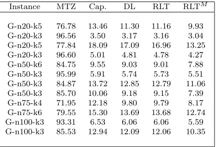
Table 2 Gap on percentage for the deterministic models
Instance MTZ Cap. DL RLT RLTM
G-n20-k5 76.78 13.46 11.30 11.16 9.93 G-n20-k3 96.56 3.50 3.17 3.16 3.04 G-n20-k5 77.84 18.09 17.09 16.96 13.25 G-n20-k3 96.60 5.01 4.81 4.78 4.27 G-n50-k6 84.75 9.55 9.03 9.01 7.88 G-n50-k3 95.99 5.91 5.74 5.73 5.51 G-n50-k3 84.87 13.72 12.85 12.79 11.06 G-n50-k3 85.70 10.06 9.18 9.15 7.39 G-n75-k4 71.95 12.18 9.80 9.79 8.17 G-n75-k6 79.55 15.30 13.69 13.68 12.74 G-n100-k3 93.31 6.53 6.06 6.06 5.59 G-n100-k3 85.53 12.94 12.09 12.06 10.35
would like to compare the performance of the RLT approach presented in Sec-tion 3.4 and the lifting approach presented in SecSec-tion 3.3. The first column represents the instances. For example, G-n20-k5 has 20 vertices, 5 types of vehicles and unlimited number of vehicles of each type. The second column (MTZ) corresponds to the LP relaxation of the standard MTZ formulation (1–9). The third column (Cap.) corresponds to the LP relaxation of the stan-dard MTZ formulation after adding the capacity inequalities (10). The fourth column (DL) is obtained by substituting (7) and (8) with (13) and (14) in (1–9). The fifth column (RLT) is obtained by replacing (7) and (8) with (17)– (20b). The big-M method can be used to linearize the nonlinear term in the RLT (16) as follows. The gap for the RLTM is provided in its corresponding column.
[image:17.595.135.348.229.374.2]5.2 Experiments with Demand Uncertainty
We start with describing how the data uncertainty is constructed, then we ex-plain the performance measures used and finally we analyze the computational results.
Uncertain Data To build demand uncertainty sets for the BS and BN robust models, we allowqito vary up to a fixed percentage of its nominal value so that qi∈[q0i −υq0i, qi0+υq0i], whereq0i is the demand nominal value andυ= 0.1 or 0.2. To build uncertainty sets for the CC model, it is quite common to consider a normal distribution based on the mean and the variance calculated for a sample. Hence, we assume that the demand of each customer follows the normal distributionN(µi, λ2i) withµi=qi0, and λ2i = 012.16qi0. Notice that we set the variance equal to the variance of the uniform distribution that we calculated for the RO cases. In this case, 91% of the interval defined previously is covered by the normal distribution function.
Performance Measures We compare our solutions according to three perfor-mance measures.
First, we compute theextra costEa required to pay for achieving a certain level of validity of routes:
Ea :=z a−zdet
za ×100,
where za denotes the optimal value of the uncertain model (a can bebs, bn andccfor BS, BN and CC models, respectively) andzdet is the optimal value for the deterministic case.
In case of failure, there are two possible strategies. On the one hand, one may assume that vehicles return to the depot and do not resume the inter-rupted (failed) route, so the remaining customers on the failed route are left unserved. This is known asallowed lost sales (ALS). The second performance measure represents the number of unmet customers (and the corresponding unmet demand). On the other hand, if lost sale is not allowed (NALS), the vehicle returns to the depot for a replenishment and then resumes the route starting from the first customer who was left unserved. The third performance measure calculates therecourse cost.
solution and find the thresholds at which the optimal solution will change. In many cases of MIP, a full description of the convex hall of the feasible region is not available and constraints may not define facets of the convex hull, hence changing the parameters may affect neither the optimal solution nor the objective value. On the other hand, if an optimal solution is cut off as a result of varying parameters, the effect can be dramatic from changing the optimal solution to infeasible solution. Therefore, particularly in practice when resources are limited, it is vital to define appropriate risk levels so that not only the solution is feasible but also unnecessary extra costs are not imposed. One way of identifying the threshold is to define different scenarios for the risk level. Here in addition to the nominal case which representsα0= 0.5, we
consider 9 scenarios for the risk level (α1= 0.40, α2= 0.30, α3= 0.25, α4=
0.20, α5 = 0.10, α6 = 0.05, α7 = 0.03, α8 = 0.01, α9 = 0.001). Note that
the larger the risk level, the higher the probability of violating a constraint. We solve the CCP and BS-RO deterministic counterparts of the instances for all these scenarios and calculate the aforementioned performance measures for each scenario. As formulated in the previous section, the protection level of the BS-RO (Γ) is calculated for each risk level. Then, among the risk level scenarios, the optimal one can be suggested.
Computational results In this experiment, we consider the variable routing cost for the data sets. All experiments are carried out on a Dell Precision T1600 computer with a 3.4 GHz Intel Xeon Processor and 16 GB RAM running Ubuntu Linux 12. Also note that we use our B&C method for the nominal problem and the BN-RO and the default CPLEX solver for the BS-RO. When a user defined B&C method is run in CPLEX, by default CPLEX uses only one thread.
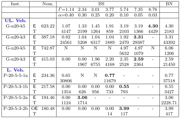
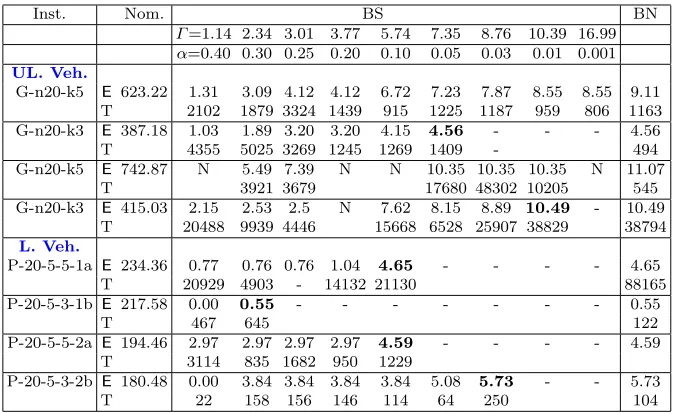
Tables 3 and 4 present Ebs and Ebn values withυ = 10% and υ = 20%, respectively. Table 5 presents Ecc values with υ = 20%. All running times are in seconds. Note that, when the BS optimal value equals the BN optimal value, we do not need to run other risk levels since they will give the same results. When this happens, we use bold numbers in Tables 3 and 4 for the corresponding percentage of extra cost.
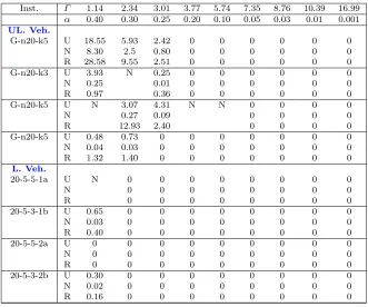
In order to calculate for the second and third performance measures, we generate random demands for all customers from their defined distribution functions to simulate the actual situations. Table 6 reports the results for the average of the second and third performance measures for 100 simulations with υ = 20%. For each instance, we use abbreviations as follows: U (Unmet De-mands), N (Number of Unmet deDe-mands), R (Recourse Cost) and NR (Number of Routes). As the numerical result suggests, we do not need to set a very low risk level to achieve 100% valid routes.
pre-defined intervals, assuming that they follow a uniform distribution (100 realizations for each demand). Since in only one scenario the risk level is zero, there is a possibility of failure for the other scenarios. First, we assume that no lost sale is allowed, so the recourse actions are performed to serve unmet customers and the related recourse costs are calculated and added to the op-timal costs obtained by the BS-RO. We call this total cost as the actual cost with recourse action. Figure 1 illustrates these three cost graphs for instance G-n20-k5. One can observe that if the risk level is set at a big value (α= 0.40), the actual cost is even less than when the risk level is very small (α≤0.10). It suggests that the extra cost paid to prevent the route validity for certain level is not necessary. In this specific problem, if the risk level is set toα= 0.20, the total cost will be minimum. We can conclude that a lower risk level does not necessarily lead to a better result. Some unnecessary costs may be imposed without any significant outcome for the system. Figure 1 and Table 8 (NALS) provide the optimal level of risk level for each problem of the BS-RO and the CCP. Obviously, the BN-RO is too conservative and imposes unnecessary costs.
On the other hand, we can assume that lost sales/unmet customers are allowed in some cost. This means when a failure occurs the vehicle returns to the depot and does not resume the route, so the remaining customers on the failed route will be left unserved. To identify the optimal risk level in this case, let us assume a simple case where each lost sale has the same cost of f. We undertake a pairwise comparison among different scenarios to find out under which condition one is better than the other. LetC1,C2,n1andn2 be
the optimal cost and the number of unmet customers for two risk scenarios 1 and 2, respectively. If (n1−n2)f ≤C2−C1, then scenario 1 is better than
scenario 2. Otherwise, scenario 2 is better than scenario 1. Therefore, a risk level can be the best scenario for a specific range of lost sale costs.
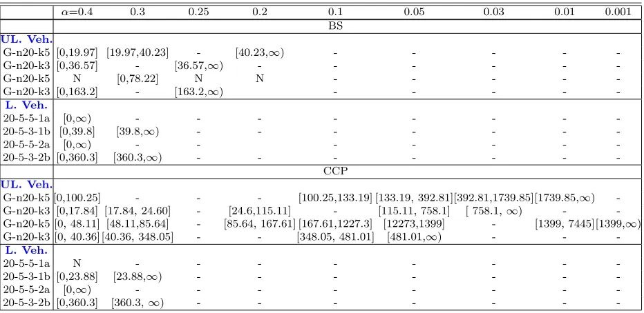
Table 9 presents intervals forf in which a risk level is the optimal when lost sales is allowed (ALS). For instance, for Instance G-n20-k5, for the BS-RO when f ∈[0, 19.97] andf ∈[19.97, 40.23], then the best risk levels are α= 0.4 and α= 0.3, respectively. However,α= 0.25 cannot be the optimal risk level as it has the same cost ofα= 0.2 while there are unmet customers. So, when f ∈ [40.23, ∞)α = 0.2 is the optimal risk level. As this analysis also suggests, the smaller risk levels are not necessarily the best options.
6 Conclusions
Robust optimization and chance constrained programming are important tools in the presence of data uncertainty. We have studied the HVRP under de-mand uncertainty. Rather than choosing a particular uncertainty model, we have considered three well-known models and analyzed them using different performance measure.
improve the branch-and-bound algorithm in order to consider larger instances. From a theoretical point of view, it would be interesting to see if the concept of risk level can be addressed more systematically, with possible consideration of bi-objective models and computingParetosolutions.
References
1. R. Baldacci, E. Bartolini, A. Mingozzi, and R. Roberti. An exact solution framework for a broad class of vehicle routing problems. Computational Management Science, 7:229–268., 2010.
2. R. Baldacci, M. Battarra, and D. Vigo. Valid inequalities for the fleet size and mix vehicle routing problem with fixed costs. Networks, 54(4):178–189, 2009.
3. R. Baldacci and A. Mingozzi. A unified exact method for solving different classes of vehicle routing problems.Math. Program., 120(2):347–380, 2009.
4. A. Ben-Tal and A. Nemirovski. Robust solutions of uncertain linear programs. Math. Program., B:1–13, 1999.
5. Dimitris Bertsimas and Melvyn Sim. The price of robustness. Operations Research, 52(1):35–53, 2004.
6. Dimitris J. Bertsimas. A vehicle routing problem with stochastic demand. Operations Research, 40(3):574–585, 1992.
7. C. E. Blair and R. G. Jeroslow. The value function of an integer program.Mathematical Programming, 23:237–273, 1982.
8. A. Charnes and W. Cooper. Chance-constrained programming. Management Science, 6:73–79, 1959.
9. A. Charnes and W. Cooper. Deterministic equivalents for optimizing and satisficing under chance-constrained. Operations Research, 11:18–39, 1963.
10. Christian H. Christiansen and Jens Lysgaard. A branch-and-price algorithm for the capacitated vehicle routing problem with stochastic demands. Operations Research Letters, 35(6):773 – 781, 2007.
11. M. Desrochers and G. Laporte. Improvements and extensions to the miller-tucker-zemlin subtour elimination constraints.Operations Research Letters, 10:27–36, 1991. 12. M. Dror. Modeling Uncertainty: An Examination of Stochastic Theory, Methods, and
Applications. International Series in Operations Research and Management Science, chapter Vehicle routing with stochastic demands: Models and computational methods, pages 625–649. Kluwer, Boston, 2002.
13. M. Dror and P. Trudeau. Stochastic vehicle routing with modified savings algorithm.
European Journal of Operational Research, 23:228–235, 1986.
14. Alan L. Erera, Juan C. Morales, and Martin Savelsbergh. The vehicle routing problem with stochastic demand and duration constraints. Transportation Science, 44:474–492, 2010.
15. Michel Gendreau, Gilbert Laporte, and Rene Seguin. Stochastic vehicle routing. Euro-pean Journal of Operational Research, 88(1):3–12, 1996.
16. B. Golden, A. Assad, L. Levy, and F. Gheysens. The fleet size and mix vehicle routing problem.Computers and Operations Research, 11:49–66, 1984.
17. G. Laporte and F. Louveaux. Formulations and bounds for the stochastic capacitated vehicle routing problem with uncertain supplies. Technical report, Ecole des Hautes Etudes Commerciale, University of Montreal, Montreal, Canada, 1987.
18. G. Laporte, F. Louveaux, and H. Mercure. Models and exact solutions for a class of stochastic location-routing problems. European Journal of Operational Research, 39:71–78, 1989.
19. G. Laporte and F.V. Louveaux. The integer l-shaped methods for stochastic integer programs with complete recourse. Oper. Res. Lett., 13:133–142, 1993.
20. Adam N. Letchford and Juan-Jose Salazar-Gonzalez. Projection results for vehicle routing.Mathematical Programming, 105:251–274, 2006. 10.1007/s10107-005-0652-x. 21. C.E. Miller, A.W. Tucker, and R.A. Zemlin. Integer programming formulations and
22. C. Novoa, R. Berger, J. Linderoth, and R. Storer. A set-partitioning-based model for the stochastic vehicle routing problem. Technical report, Lehigh University, 2006. 23. Nicola Secomandi and Francois Margot. Reoptimization approaches for the
vehicle-routing problem with stochastic demands.Operations Research, 57(1):214–230, 2009. 24. H.D. Sherali and W. Adams. A hierarchy of relaxations between the continuous and
con-vex hull representations for zero-one programming problems.Siam Journal of Discrete Mathematics, 3:411–430, 1990.
25. H.D. Sherali and P.J. Driscoll. On tightening the relaxations of miller-tucker-zemlin formulations for asymmetric traveling salesman problems.Operations Research, 50:656– 669., 2002.
26. William R. Stewart and Bruce L. Golden. Stochastic vehicle routing: A comprehensive approach.European Journal of Operational Research, 14(4):371 – 385, 1983.
27. Ilgaz Sungur, Fernando Ordez, and Maged Dessouky. A robust optimisation approach for the capacitated vehicle routing problem with demand uncertainty.IIE Transactions, 40:509–523, 2008.
28. Frank A. Tillman. The multiple terminal delivery problem with probabilistic demands.
Transportation Science, 3:192–204, 1969.
[image:22.595.82.398.323.532.2]29. Hande Yaman. Formulations and valid inequalities for the heterogeneous vehicle routing problem.Math. Program., A 106:365–390, 2006.
Table 3 The deterministic optimal objective value and the first performance measure for BS-RO and BN-RO (υ= 0.1), where N indicates unsolved.
Inst. Nom. BS BN
Γ=1.14 2.34 3.01 3.77 5.74 7.35 8.76 α=0.40 0.30 0.25 0.20 0.10 0.05 0.03
UL. Veh.
G-n20-k5 E 623.22 1.07 1.33 1.45 1.91 3.19 3.19 4.30 4.30 T 4147 2199 1264 859 2103 1366 4429 2183 G-n20-k3 E 387.18 0.82 1.04 1.04 1.04 1.92 3.31 - 3.31 T 24561 5208 6317 1889 2470 29387 43392 G-n20-k5 E 742.87 N N N N 4.97 4.97 N 6.06
T 5632 1079 1206
G-n20-k3 E 415.03 0.00 0.00 1.96 2.20 2.35 2.59 - 2.59
T 1967 6755 4168 2528 2364 21450
L. Veh.
P-20-5-5-1a E 234.36 0.65 N N 0.77 - - - 0.77
T 30806 11679 37518
P-20-5-3-1b E 217.58 0.00 0.00 0.00 0.00 0.55 - - 0.55
T 1354 626 956 733 793 3427
P-20-5-5-2a E 194.46 0.00 3.06 - - - 3.06
T 1124 1714 2228.71
P-20-5-3-2b OE 180.48 0.00 0.00 0.00 0.00 3.99 - - 3.99
Table 4 The deterministic optimal objective value and the first performance measure for BS-RO and BN-RO (υ= 0.2)
Inst. Nom. BS BN
Γ=1.14 2.34 3.01 3.77 5.74 7.35 8.76 10.39 16.99 α=0.40 0.30 0.25 0.20 0.10 0.05 0.03 0.01 0.001
UL. Veh.
G-n20-k5 E 623.22 1.31 3.09 4.12 4.12 6.72 7.23 7.87 8.55 8.55 9.11 T 2102 1879 3324 1439 915 1225 1187 959 806 1163 G-n20-k3 E 387.18 1.03 1.89 3.20 3.20 4.15 4.56 - - - 4.56
T 4355 5025 3269 1245 1269 1409 - 494
G-n20-k5 E 742.87 N 5.49 7.39 N N 10.35 10.35 10.35 N 11.07
T 3921 3679 17680 48302 10205 545
G-n20-k3 E 415.03 2.15 2.53 2.5 N 7.62 8.15 8.89 10.49 - 10.49 T 20488 9939 4446 15668 6528 25907 38829 38794
L. Veh.
P-20-5-5-1a E 234.36 0.77 0.76 0.76 1.04 4.65 - - - - 4.65
T 20929 4903 - 14132 21130 88165
P-20-5-3-1b E 217.58 0.00 0.55 - - - 0.55
T 467 645 122
P-20-5-5-2a E 194.46 2.97 2.97 2.97 2.97 4.59 - - - - 4.59 T 3114 835 1682 950 1229
P-20-5-3-2b E 180.48 0.00 3.84 3.84 3.84 3.84 5.08 5.73 - - 5.73
T 22 158 156 146 114 64 250 104
Table 5 The deterministic optimal objective value and the first performance measure for CCP (υ= 0.2)
Nom. CCP
Inst. α= 0.40 0.30 0.25 0.20 0.10 0.05 0.03 0.01 0.001
UL. Veh.
G-n20-k5 E 623.22 2.72 6.84 8.80 10.01 18.81 24.79 29.21 34.79 41.73
T 278 190 69 37 102 40 21 25 6
G-n20-k3 E 387.18 2.56 4.27 5.09 5.16 11.63 14.65 17.51 19.87 28.92 T 1287 864 402 132 312 172 212 118 38 G-n20-k5 E 742.87 5.87 10.21 14.01 14.01 24.17 32.43 38.08 43.16 58.12
T 2622 293 2096 264 1674 242 532 53 22 G-n20-k3 E 415.03 2.20 8.52 10.23 11.41 17.75 24.70 27.89 31.09 38.73
T 509 3435 2472 1044 389 408 547 257 38
L. Veh.
P-20-5-5-1a E 234.36 N N N N N N N N N
T
P-20-5-3-1b E 217.58 0.00 0.55 0.55 0.55 0.98 6.62 6.62 12.03 13.23 T 786 408 195 139 162 399 295 1197 694 P-20-5-5-2a jE 194.46 3.06 3.06 4.81 4.81 7.10 7.10 15.41 18.19 21.95
[image:23.595.83.396.358.556.2]Γ(α) Gap (%)
3.77(0.2)* 0(0.5)
9.11
20(0) 5.92
BS BN
actual
[image:24.595.72.398.79.235.2]Fig. 1 Risk levels, optimal costs and actual costs for Instance G-n20-k5
Table 6 Second and third performance measures for the BS (υ= 0.2)
Inst. Γ 1.14 2.34 3.01 3.77 5.74 7.35 8.76 10.39 16.99 α 0.40 0.30 0.25 0.20 0.10 0.05 0.03 0.01 0.001
UL. Veh.
G-n20-k5 U 18.55 5.93 2.42 0 0 0 0 0 0
N 8.30 2.5 0.80 0 0 0 0 0 0
R 28.58 9.55 2.51 0 0 0 0 0 0
G-n20-k3 U 3.93 N 0.25 0 0 0 0 0 0
N 0.25 0.01 0 0 0 0 0 0
R 0.97 0.36 0 0 0 0 0 0
G-n20-k5 U N 3.07 4.31 N N 0 0 0 0
N 0.27 0.09 0 0 0 0
R 12.93 2.40 0 0 0 0
G-n20-k5 U 0.48 0.73 0 0 0 0 0 0 0
N 0.04 0.03 0 0 0 0 0 0 0
R 1.32 1.40 0 0 0 0 0 0 0
L. Veh.
20-5-5-1a U N 0 0 0 0 0 0 0 0
N 0 0 0 0 0 0 0 0
R 0 0 0 0 0 0 0 0
20-5-3-1b U 0.65 0 0 0 0 0 0 0 0
N 0.03 0 0 0 0 0 0 0 0
R 0.40 0 0 0 0 0 0 0 0
20-5-5-2a U 0 0 0 0 0 0 0 0 0
N 0 0 0 0 0 0 0 0 0
R 0 0 0 0 0 0 0 0 0
20-5-3-2b U 0.30 0 0 0 0 0 0 0 0
N 0.02 0 0 0 0 0 0 0 0
[image:24.595.75.406.284.560.2]Table 7 Second and third performance measures for the CCP (υ= 0.2)
Inst. Γ 1.14 2.34 3.01 3.77 5.74 7.35 8.76 10.39 16.99 α 0.40 0.30 0.25 0.20 0.10 0.05 0.03 0.01 0.001
UL. Veh.
G-n20-k5 U 46.96 52.55 43.72 43.01 20.62 4.32 1.89 0 0 N 1.37 1.25 0.99 1.00 0.37 0.09 0.02 0 0 R 42.88 46.96 31.93 35.41 13.07 3.12 0.59 0 0 G-n20-k3 U 19.12 16.05 13.16 16.99 1.62 1.43 0 0 0
N 0.75 0.38 0.25 0.31 0.03 0.03 0 0 0
R 20.51 11.87 7.63 8.9 1 1.33 0 0 0
G-n20-k5 U 49.21 37.07 29.38 25.38 5.48 4.52 1.20 1.19 0 N 1.64 0.97 0.64 0.55 0.1 0.05 0.02 0.03 0 R 50.79 39.3 23.29 23.05 4.85 1.89 1.14 1.63 0
G-n20-k5 U 40.8 4.56 6.03 17.46 3.24 0 0 0 0
N 0.82 0.17 0.20 0.30 0.06 0 0 0 0
R 34.36 6.91 9.04 9.26 1.90 0 0 0 0
UL. Veh.
20-5-5-1a U N N N N N N N N N
N R
20-5-3-1b U 1.05 0 0 0 0 0 0 0 0
N 0.05 0 0 0 0 0 0 0 0
R 0.67 0 0 0 0 0 0 0 0
20-5-5-2a U 0 0 0 0 0 0 0 0 0
N 0 0 0 0 0 0 0 0 0
R 0 0 0 0 0 0 0 0 0
20-5-3-2b U 0.32 0 0 0 0 0 0 0 0
N 0.02 0 0 0 0 0 0 0 0
R 0.16 0 0 0 0 0 0 0 0
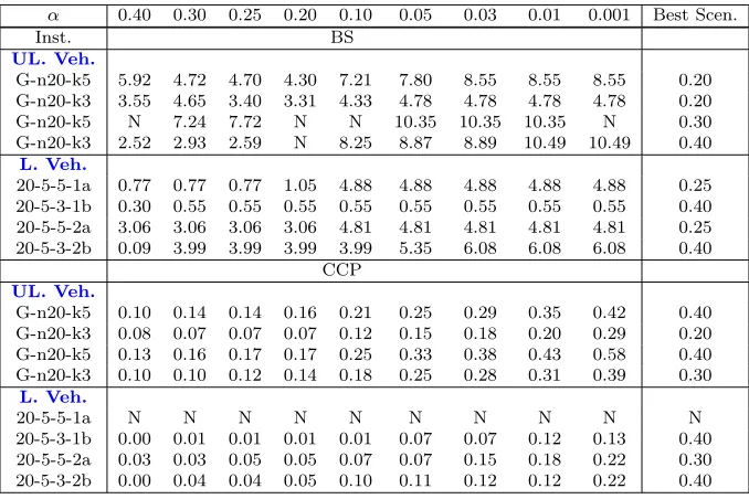
Table 8 Best scenario for the risk level when lost sales are not allowed for BS and CCP
α 0.40 0.30 0.25 0.20 0.10 0.05 0.03 0.01 0.001 Best Scen.
Inst. BS
UL. Veh.
G-n20-k5 5.92 4.72 4.70 4.30 7.21 7.80 8.55 8.55 8.55 0.20 G-n20-k3 3.55 4.65 3.40 3.31 4.33 4.78 4.78 4.78 4.78 0.20 G-n20-k5 N 7.24 7.72 N N 10.35 10.35 10.35 N 0.30 G-n20-k3 2.52 2.93 2.59 N 8.25 8.87 8.89 10.49 10.49 0.40
L. Veh.
20-5-5-1a 0.77 0.77 0.77 1.05 4.88 4.88 4.88 4.88 4.88 0.25 20-5-3-1b 0.30 0.55 0.55 0.55 0.55 0.55 0.55 0.55 0.55 0.40 20-5-5-2a 3.06 3.06 3.06 3.06 4.81 4.81 4.81 4.81 4.81 0.25 20-5-3-2b 0.09 3.99 3.99 3.99 3.99 5.35 6.08 6.08 6.08 0.40
CCP
UL. Veh.
G-n20-k5 0.10 0.14 0.14 0.16 0.21 0.25 0.29 0.35 0.42 0.40 G-n20-k3 0.08 0.07 0.07 0.07 0.12 0.15 0.18 0.20 0.29 0.20 G-n20-k5 0.13 0.16 0.17 0.17 0.25 0.33 0.38 0.43 0.58 0.40 G-n20-k3 0.10 0.10 0.12 0.14 0.18 0.25 0.28 0.31 0.39 0.30
L. Veh.
20-5-5-1a N N N N N N N N N N
[image:25.595.72.411.407.633.2]Table 9 Best intervals of the lost sale cost for each scenario for the BS and the CCP
α=0.4 0.3 0.25 0.2 0.1 0.05 0.03 0.01 0.001
BS
UL. Veh.
G-n20-k5 [0,19.97] [19.97,40.23] - [40.23,∞) - - - -
-G-n20-k3 [0,36.57] - [36.57,∞) - - -
-G-n20-k5 N [0,78.22] N N - - - -
-G-n20-k3 [0,163.2] - [163.2,∞) - - - -
-L. Veh.
20-5-5-1a [0,∞) - - -
-20-5-3-1b [0,39.8] [39.8,∞) - - -
-20-5-5-2a [0,∞) - - -
-20-5-3-2b [0,360.3] [360.3,∞) - - -
-CCP
UL. Veh.
G-n20-k5 [0,100.25] - - - [100.25,133.19] [133.19, 392.81][392.81,1739.85][1739.85,∞)
-G-n20-k3 [0,17.84] [17.84, 24.60] - [24.6,115.11] - [115.11, 758.1] [ 758.1,∞) -
-G-n20-k5 [0, 48.11] [48.11,85.64] - [85.64, 167.61] [167.61,1227.3] [12273,1399] - [1399, 7445][1399,∞)
G-n20-k3 [0, 40.36] [40.36, 348.05] - - [348.05, 481.01] [481.01,∞) - - -L. Veh.
20-5-5-1a N - - -
-20-5-3-1b [0,23.88] [23.88,∞) - - -
-20-5-5-2a [0,∞) - - -