Representing Text Chunks

(1)

Representing Text Chunks

E r i k F . T j o n g K i m S a n g C e n t e r for D u t c h L a n g u a g e a n d Speech

U n i v e r s i t y of A n t w e r p U n i v e r s i t e i t s p l e i n 1 B-2610 W i l r i j k , B e l g i u m

e r i k t @ u i a . a c . b e

J o r n

V e e n s t r a C o m p u t a t i o n a l L i n g u i s t i c s

T i l b u r g U n i v e r s i t y P.O. B o x 90153

5000 L E T i l b u r g , T h e N e t h e r l a n d s v e e n s t r a @ k u b . n l

A b s t r a c t

Dividing sentences in chunks of words is a useful preprocessing step for parsing, information extraction and information retrieval. (l~mshaw and Marcus, 1995) have introduced a "convenient" data representation for chunking by converting it to a tagging task. In this paper we will examine seven different data representations for the problem of recognizing noun phrase chunks. We will show that the the data representation choice has a minor influence on chunking performance. However, equipped with the most suitable data representation, our memory-based learning chunker was able to improve the best published chunking results for a standard data set.

1 I n t r o d u c t i o n

The text corpus tasks parsing, information extraction and information retrieval can benefit from dividing sentences in chunks of words. (Ramshaw and Marcus, 1995) describe an error-driven transformation-based learning (TBL) method for finding NP chunks in texts. NP chunks (or baseNPs) are non-overlapping, non-recursive noun phrases. In their experiments they have modeled chunk recognition as a tagging task: words that are inside a baseNP were marked I, words outside a baseNP received an 0 tag and a special tag B was used for the first word inside a baseNP immediately following another baseNP. A text example:

original:

In [N early trading N] in [N Hong Kong N] [N Monday N], [N gold N] was quoted at [N $ 366.50

N]

[N an ounce g] • tagged:

In/O early/I trading/I in/O Hong/I

Kong/I Monday/B ,/O gold/I was/O quoted/O at/O $/I 366.50/I an/B ounce/I ./O

Other representations for NP chunking can be used as well. An example is the representation used in (Ratnaparkhi, 1998) where all the chunk- initial words receive the same start tag (analo- gous to the B tag) while the remainder of the words in the chunk are paired with a different tag. This removes tagging ambiguities. In the Ratna- parkhi representation equal noun phrases receive the same tag sequence regardless of the context in which they appear.

The data representation choice might influence the performance of chunking systems. In this paper we discuss how large this influence is. There- fore we will compare seven different data representation formats for the baseNP recognition task. We are particularly interested in finding out whether with one of the representation formats the best reported results for this task can be improved. The second section of this paper presents the general setup of the experiments. The results Can be found in the third section. In the fourth section we will describe some related work. 2 M e t h o d s a n d e x p e r i m e n t s

In this section we present and explain the data representation formats and the machine learning algorithm that we have used. In the final part we describe the feature representation used in our experiments.

2.1 D a t a

representation

(2)

IOB1 O I I O I I B O I O O O I I B I O

IOB2 O B I O B I B O B O O O B I B I O

IOE1 O I I O I E I O I O O O I E I I O

IOE2 O I E O I E E O E O O O I E I E O

IO I O I I O I I I O I O O O I I I I O

[

]

Table 1: T h e chunk tag sequences for the example sentence I n early trading in H o n g K o n g M o n d a y , gold was quoted at $ 366.50 an ounce . for seven different tagging formats. T h e I tag has been used for words inside a baseNP, [:1 for words outside a baseNP, B and [ for baseNP-initial words a n d E and ] for baseNP-final words.

in their t r e a t m e n t of chunk-initial and chunk-final [ + ] words:

IOB1

IOB2 IOE1

IOE2

T h e first word inside a baseNP immediately following another baseNP receives a B tag (Ramshaw and Marcus, 1995).

All baseNP-initial words receive a B tag (Ratnaparkhi, 1998). T h e final word inside a baseNP immediately preceding another baseNP receives an E tag. All baseNP-final words receive an E tag.

We wanted to compare these d a t a representation tbrmats with a standard bracket representation. We have chosen to divide bracketing experiments in two parts: one for recognizing opening brackets and one for recognizing closing brackets. Additionally we have worked with another partial representation which seemed promising: a tagging representation which disregards boundaries between adjacent chunks. These boundaries can be recovered by combining this format with one of the bracketing formats. O u r three partial rep- rcsentations are:

[ All baseNP-initial words receive an [ tag, other words receive a . tag. ] All t)aseNP-final words receive a ]

tag, other words receive a . tag. IO Words inside a b a s e N P receive an I

tag, others receive an

O

tag.

These partial representations can be combined ill three pairs which encode the complete baseNP structure, of tile data:

[+IO

I0+]

A word sequence is regarded as a b a s e N P if the first word has received an [ tag, the final word has received a ] t a g and these are the only brackets t h a t have been assigned to words in the sequence. In the IO f o r m a t , tags of words t h a t have received an I t a g a n d an [ t a g are changed into B tags. T h e result is interpreted as the I O B 2 format.

In the IO format, tags of words t h a t have received an I t a g a n d a ] t a g axe changed into E tags. T h e result is interpreted as the I O E 2 format.

Examples of the four complete f o r m a t s and the three partial f o r m a t s can be found in table 1. 2.2 M e m o r y - B a s e d L e a r n i n g

We have build a b a s e N P recognizer by training a machine learning algorithm with correct tagged d a t a and testing it with unseen data. T h e machine learning algorithm we used was a Memory- Based Learning algorithm (MBL). During training it stores a symbolic feature representation of a word in the training d a t a together with its classification (chunk tag). In the testing phase the algo- r i t h m compares a feature representation of a test word with every training d a t a item and chooses the classification of the training item which is closest to the test item.

In the version of the algorithm t h a t we have

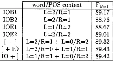
[image:2.596.116.480.82.169.2]

(3)

w o r d / P O S context IOB1 L = 2 / R = I IOB2 L = 2 / R = I IOE1 L = I / R = 2 IOE2 L = 2 / R = 2

[ + ]

L=2/R=I + L=O/R=2

[ + IO

L=2/R=O + L=I/R=I

IO + ]

L=I/R=I + L=O/R=2

F~3=l 89.17 88.76 88.67 89.01 89.32 89.43 89.42

Table 2: Results first experiment series: the best F~=I scores for different left (L) and right (R) w o r d / P O S tag pair context sizes for the seven representation formats using 5-fold cross-validation on section 15 of the WSJ corpus.

normalized entropy decrease of the classification set caused by the presence of the feature. Details of the algorithm can be found in (Daelemans et

al., 1998) I.

2.3 R e p r e s e n t i n g words with f e a t u r e s An i m p o r t a n t decision in an MBL experiment is the choice of the features t h a t will be used for representing the data. IBI-IG is thought to be less sensitive to redundant features because of the data-dependent feature weighting that is included in the algorithm. We have found that the presence of redundant features has a negative influence on the performance of the baseNP recognizer.

In (Ramshaw and Marcus, 1995) a set of trans- formational rules is used for modifying the classification of words. The rules use context information of the words, the part-of-speech tags t h a t have been assigned to them and the chunk tags t h a t are associated with them. We will use the same information as in our feature representation for words.

In TBL, rules with different context information are used successively for solving different prob- lems. We will use the same context information for all data. The optimal context size will be determined by comparing the results of different context sizes on the training data. Here we will perform four steps. We will s t a r t with testing dif- fhrent context sizes of words with their part-of- speech tag. After this, we will use the classification results of the best context size for determining the optimal context size for the classification tags. As a third step, we will evaluate combinations of classification results and find the best combina- tion. Finally we will examine the influence of an MBL algorithm parameter: the number of exam- ined nearest neighbors.

~lr~l-l(; is a part of the TiMBL software package which is available from http://ilk.kub.nl

3 R e s u l t s

We have used the baseNP d a t a presented in (Ramshaw and Marcus, 1995) 2. This d a t a was divided in two parts. The first part was training d a t a and consisted of 211727 words taken from sections 15, 16, 17 and 18 from the Wall Street Journal corpus (WSJ). T h e second p a r t was test d a t a and consisted of 47377 words taken from section 20 of the same corpus. The words were part-of-speech (POS) tagged with the Brill tagger and each word was classified as being inside or outside a baseNP with the IOB1 representation scheme. The chunking classification was m a d e by (Ramshaw and Marcus, 1995) based on the parsing information in the W S J corpus.

T h e performance of the baseNP recognizer can be measured in different ways: by computing the percentage of correct classification tags (accuracy), the percentage of recognized baseNPs t h a t are correct (precision) and the percentage of baseNPs i n t h e corpus t h a t are found (recall). We will follow (Argamon et al., 1998) and use a com- bination of the precision and recall rates: F~=I = (2" precision*recall) / (precision+recall).

In our first experiment series we have tried to discover the best word/part-of-speech tag context for each representation format. For c o m p u t a t i o n a l reasons we have limited ourselves to working with section 15 of the W S J corpus. This section contains 50442 words. We have run 5-fold cross- validation experiments with all combinations of left and right contexts of w o r d / P O S tag pairs in the size range 0 to 4. A s u m m a r y of the results can be found in table 2.

[image:3.596.201.384.78.178.2]

(4)

w o r d / P O S context chunk tag context IOB1 L = 2 / R = I

IOB2 L - - 2 / R = I

IOE1

L=I/R=2

IOE2 L = I / R = 2 [ + ] L = 2 / R = I + L = 0 / R = 2

[

+ IO L=2/R=0 + L=I/R=I

IO + ] L = I / R = I + L = 0 / R = 2

F~=I

1/2 90.12

1/0

89.30

1/2 89.55

0/1 89.73

0/0 + 0/0 89.32 0/0 +

I / I

89.78 1/1 + 0/0 89.86

Table 3: Results second experiment series: the best F~=I scores for different left (L) and right (R) chunk tag context sizes for the seven representation formats using 5-fold cross-validation on section 15 of the WSJ corpus.

w o r d / P O S chunk tag combinations

IOB1 2/1

IOB2 2/1

IOE1 1/2

IOE2 1/2

[ + ]

2 / 1 + 0 / 2

[ + IO 2/0 +

1/1

IO+] I/1+0/2

I / i

1/o

1/2

o/i

o/o + o/o

0/0 -F

I / I

1/1 -F 0/0

F~=I

0/0 1/1 2/2 3/3 90.53

2/1 89.30

0/0 1/1 2/2 3/3

90.03

1/2 89.73

+ 89.32

- + 0/1 1/2 2/3 3 / 4 89.91

0/1 1/2 2/3 3/4 + -

90.03

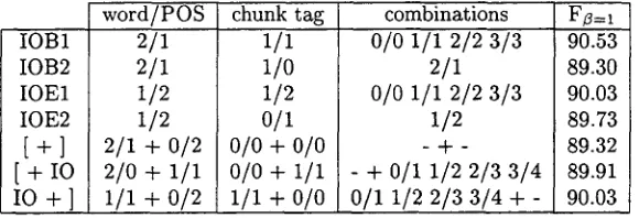
Table 4: Results third experiment series: the best F~=I scores for different combinations of chunk tag context sizes for the seven representation formats using 5-fold cross-validation on section 15 of the WSJ corpus.

with explicit open bracket information preferred larger left context and most formats with explicit closing b r a c k e t information preferred larger right context size. The three combinations of partial representations systematically outperformed the four complete representations. This is probably caused by the fact that they are able to use two different context sizes for solving two different parts of the recognition problem.

In a second series of experiments we used a "cascaded" classifier. This classifier has two stages (cascades). T h e first cascade is similar to the clas- sifter described in the first experiment. For the second cascade we added the classifications of the first cascade as extra features. T h e e x t r a features consisted of the left and the right context of the classification tags. The focus chunk tag (the classification of the current word) accounts for the correct classification in about 95% of the cases. The MBL algorithm assigns a large weight to this input feature and this makes it harder for the other features to contribute to a good result. To avoid this we have refrained from using this tag. Our goal was to find out the optimal number of extra classification tags in the input. We performed 5-fold cross-validation experiments with all combinations of left, and right classification tag contexts in the range 0 tags to 3 tags. A summary of

the results can be found in table 33 . We achieved higher F~=I for all representations except for the bracket pair representation.

The third experiment series was similar to the second but instead of adding o u t p u t of one experiment we added classification results of three, four or five experiments of the first series. By do- ing this we supplied the learning algorithm with information about different context sizes. This information is available to T B L in the rules which use different contexts. We have limited ourselves to examining all successive combinations of three, four and five experiments of the lists

(L=O/R=O,

1/1, 2/2, 3/3, 4/4), (0/1, 1/2, 2/3, 3/4) and (1/0, 2/1, 3/2, 4/3). A summary of the results can be found in table 4. The results for four representation formats improved.

[image:4.596.153.443.81.181.2] [image:4.596.155.445.239.338.2]

(5)

word/POS chunk tag combinations FB=I

IOB1

3/3(k=3)

IOB2

3/3(k=3)

IOE1

2/3(k=3)

IOE2

2/3(k=3)

[ + ]

4/3(3) + 4/4(3)

[ + IO 4/3(3) + 3/3(3)

IO + ]

3/3(3) + 2/3(3)

1/1

1/o

1/2

o/1

o/o + o/o

0/0 + 1/1

1/1 + OlO

0/0(1) 1/1(1) 2/2(3) 3/3(3) 3/3(3)

0/0(1) 1/1(1) 2/2(3) 3/3(3) 2/3(3)

- + 0/1(1) 1/2(3) 2/3(3) 3/4(3) 0/1(1) 1/2(3) 2/3(3) 3/4(3) + -

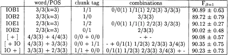
90.89 + 0.63 89.72 4- 0.79 90.12 + 0.27 90.02 4- 0.48 90.08 4- 0.57 90.35 4- 0.75 90.23 4- 0.73 Table 5: Results fourth experiment series: the best FZ=I scores for different combinations of left and right classification tag context sizes for the seven representation formats using 5-fold cross-validation on section 15 of the WSJ corpus obtained with IBI-Ic parameter k=3. IOB1 is the best representation format but the differences with the results of the other formats are not significant.

item. However (Daelemans et al., 1999) report that for baseNP recognition better results can be obtained by making the algorithm consider the classification values of the three closest training items. We have tested this by repeating the first experiment series and part of the third experiment series for k=3. In this revised version we have repeated the best experiment of the third series with the results for k = l replaced by the k=3 results whenever the latter outperformed the first in the revised first experiment series. The results can be found in table 5. All formats benefited from this step. In this final experiment series the best results were obtained with IOB1 but the differences with the results of the other formats are not significant.

We have used the optimal experiment configura- tions that we had obtained from the fourth experiment series for processing the complete (Ramshaw and Marcus, 1995) data set. The results can be found in table 6. They are better than the results for section 15 because more training data was used in these experiments. Again the best result was obtained with IOB1 (F~=I =92.37) which is an im- I)rovement of the best reported F,~=1 rate for this data set ((Ramshaw and Marcus, 1995): 92.03).

We would like to apply our learning approach to the large d a t a set mentioned in (Ramshaw and Marcus, 1995): Wall Street Journal corpus sections 2-21 as training material and section 0 as test material. With our present hardware apply- ing our optimal experiment configuration to this d a t a would require several months of computer time. Therefore we have only used the best stage 1 approach with IOB1 tags: a left and right con- t(,.xt of three words and three POS tags combined with k=3. This time the chunker achieved a F~=l score of 93.81 which is half a point better than the results obtained by (Ramshaw and Marcus, 1995): 93.3 (other chunker rates for this data: accuracy: 98.04%; precision: 93.71%; recalh 93.90%).

4 R e l a t e d w o r k

The concept of chunking was introduced by Ab- ney in (Abney, 1991). He suggested to develop a chunking parser which uses a two-part syntac- tic analysis: creating word chunks (partial trees) and attaching the chunks to create complete syn- tactic trees. Abney obtained support for such a chunking stage from psycholinguistic literature.

Ramshaw and Marcus used transformation- based learning (TBL) for developing two chunkers (Ramshaw and Marcus, 1995). One was trained to recognize baseNPs and the other was trained to recognize both NP chunks and VP chunks. Ramshaw and Marcus approached the chunking task as a tagging problem. Their baseNP training and test data from the Wall Street Journal corpus are still being used as benchmark d a t a for current chunking experiments. (Ramshaw and Marcus, 1995) shows that baseNP recognition (Fz=I =92.0) is easier than finding both NP and VP chunks (Fz=1=88.1) and t h a t increasing the size of the training data increases the performance on the test set.

[image:5.596.94.489.82.178.2]

(6)

IOB1 IOB2 IOE1 IOE2

[+]

[ + IO

IO +]

(Ramshaw and Marcus, 1995) (Veenstra, 1998) (Argamon et al., 1998) (Cardie and Pierce, 1998)

accuracy 97.58% 96.50% 97.58% 96.77%

97.37% 97.2%

precision 92.50% 91.24% 92.41% 91.93% 93.66% 91.47% 91.25% 91.80% 89.0% 91.6 % 90.7%

recall F~=I 92.25% 92.37 92.32% 91.78 92.04% 92.23 92.46% 92.20 90.81% 92.22 92.61% 92.04 92.54% 91.89 92.27% 92.03 94.3% 91.6 91.6% 91.6 91.1% 90.9

Table 6: T h e F~=I scores for the (Ramshaw and Marcus, 1995) test set after training with their training d a t a set. T h e data was processed with the optimal input feature combinations found in the fourth experiment series. The accuracy rate contains the fraction of chunk tags t h a t was correct. The other three rates regard baseNP recognition. The b o t t o m part of the table shows some other reported results with this data set. With all but two formats IBI-IG achieves better FZ=l rates than the best published result in (Ramshaw and Marcus, 1995).

(Veenstra, 1998) uses cascaded decision tree learning (IGTree) for baseNP recognition. This algorithm stores context information of words, POS tags and chunking tags in a decision tree and clas- sifies new items by comparing them to the training items. The algorithm is very fast and it reaches the same performance as (Argamon et al., 1998) (F,~=1=91.6). (Daelemans et al., 1999) uses cascaded MBL (IBI-IG) in a similar way for several tasks among which baseNP recognition. T h e y do not report F~=~ rates but their tag accuracy rates are a lot b e t t e r than accuracy rates reported by others. However, they use the (Ramshaw and Marcus, 1995) d a t a set in a different training-test division (10-fold cross validation) which makes it (tifficult to compare their results with others. 5 C o n c l u d i n g r e m a r k s

We hay('. (:omI)ared seven (tiffi~rent (tata. formats for the recognition of baseNPs with memory-based learning (IBI-IG). The IOB1 format, introduced in (Ramshaw and Marcus, 1995), consistently (:ame out as the best format. However, the differences with other formats were not significant. Some representation formats achieved better pre- (:ision rates, others better recall rates. This information is usefifl ibr tasks that require chunking structures because some tasks might be more interested in high precision rates while others might be more interested in high recall rates.

The IBI-IG algorithm has been able to improve the best reported F2=1 rates for a stan- (lar(l data set (92.37 versus (Ramshaw and Mar- (:us, 1995)'s 92.03). This result was aided by us-

ing non-standard parameter values (k=3) and the algorithm was sensitive for redundant input features. This means that finding an optimal performance or this task requires searching a large p a r a m e t e r / f e a t u r e configuration space. An inter- esting topic for future research would be to embed ml-IG in a standard search algorithm, like hill- climbing, and explore this parameter space. Some more room for improved performance lies in computing the POS tags in the d a t a with a b e t t e r tagger than presently used.

R e f e r e n c e s

Steven Abney. 1991. Parsing by chunks. In Principle-Based Parsing. Kluwer Academic Publishers,.

Shlomo Argamon, Ido Dagan, and Yuval Kry- molowski. 1998. A memory-based approach to learning shallow natural language patterns. In

Proceedings of the 17th International Confer- ence on Computational Linguistics (COLING- ACL '98).

Claire Cardie and David Pierce. 1998. Error- driven pruning of treebank grammars for base noun phrase identification. In Proceedings of the 17th International Conference on Compu- tational Linguistics (COLING-ACL '98).

Walter Daelemans, Jakub Zavrel, Ko van der Sloot, and Antal van d e n Bosch. 1998.

[image:6.596.127.458.78.226.2]

(7)

Walter Daelemans, Antal van den Bosch, and Jakub Zavrel. 1999. Forgetting exceptions is harmful in language learning. Machine Learn-

ing, 11.

Lance A. Ramshaw and Mitchell P. Marcus. 1995. Text chunking using transformation- based learning. In Proceedings of the Third A CL Workshop on Very Large Corpora.

Adwait Ratnaparkhi. 1998. Maximum Entropy Models for Natural Language Ambiguity Reso-

lution. PhD thesis Computer and Information

Science, University of Pennsylvania.

Jorn Veenstra. 1 9 9 8 . Fast np chunking using memory-based learning techniques. In

BENELEARN-98: Proceedings of the Eigth

Belgian-Dutch Conference on Machine Learn-