Proceedings of the 2011 Conference on Empirical Methods in Natural Language Processing, pages 941–948,
Entire Relaxation Path for Maximum Entropy Problems
Moshe Dubiner Google
Yoram Singer Google
Abstract
We discuss and analyze the problem of find-ing a distribution that minimizes the relative entropy to a prior distribution while satisfying max-norm constraints with respect to an ob-served distribution. This setting generalizes the classical maximum entropy problems as it relaxes the standard constraints on the ob-served values. We tackle the problem by in-troducing a re-parametrization in which the unknown distribution is distilled to a single scalar. We then describe a homotopy between the relaxation parameter and the distribution characterizing parameter. The homotopy also reveals an aesthetic symmetry between the prior distribution and the observed distribu-tion. We then use the reformulated problem to describe a space and time efficient algorithm for tracking the entire relaxation path. Our derivations are based on a compact geomet-ric view of the relaxation path as a piecewise linear function in a two dimensional space of the relaxation-characterization parameters. We demonstrate the usability of our approach by applying the problem to Zipfian distribu-tions over a large alphabet.
1 Introduction
Maximum entropy (max-ent) models and its dual counterpart, logistic regression, is a popular and ef-fective tool in numerous natural language process-ing tasks. The principle of maximum entropy was spelled out explicitly by E.T. Jaynes (1968). Ap-plications of maximum entropy approach to natural language processing are numerous. A notable ex-ample and probably one of the earliest usages and
generalizations of the maximum entropy principle to language processing is the work of Berger, Della Pietra×2, and Lafferty (Berger et al., 1996, Della Pietra et al., 1997). The original formulation of max-ent cast the problem as the task of finding the distribution attaining the highest entropy subject to equality constraints. While this formalism is aes-thetic and paves the way to a simple dual in the form of a unique Gibbs distribution (Della Pietra et al., 1997), it does not provide sufficient tools to deal with input noise and sparse representation of the target Gibbs distribution. To mitigate these issues, numerous relaxation schemes of the equality con-straints have been proposed. A notable recent work by Dudik, Phillips, and Schapire (2007) provided a general constraint-relaxation framework. See also the references therein for an in depth overview of other approaches and generalizations of max-ent. The constraint relaxation surfaces a natural param-eter, namely, a relaxation value. The dual form of this free parameter is the regularization value of pe-nalized logistic regression problems. Typically this parameter is set by experimentation using cross val-idation technique. The relaxed maximum-entropy problem setting is the starting point of this paper.
In this paper we describe and analyze a frame-work for efficiently tracking the entire relaxation path of constrained max-ent problems. We start in Sec. 2 with a generalization in which we discuss the problem of finding a distribution that minimizes the relative entropy to a given prior distribution while satisfying max-norm constraints with respect to an observed distribution. In Sec. 3 we tackle the prob-lem by introducing a re-parametrization in which the
unknown distribution is distilled to a single scalar. We next describe in Sec. 4 a homotopy between the relaxation parameter and the distribution character-izing parameter. This formulation also reveals an aesthetic symmetry between the prior distribution and the observed distribution. We use the reformu-lated problem to describe in Secs. 5-6 space and time efficient algorithms for tracking the entire relaxation path. Our derivations are based on a compact ge-ometric view of the relaxation path as a piecewise linear function in a two dimensional space of the relaxation-characterization parameters. In contrast to common homotopy methods for the Lasso Os-borne et al. (2000), our procedure for tracking the max-ent homotopy results in an uncharacteristically low complexity bounds thus renders the approach applicable for large alphabets. We provide prelim-inary experimental results with Zipf distributions in Sec. 8 that demonstrate the merits of our approach. Finally, we conclude in Sec. 9 with a brief discus-sion of future directions.
2 Notations and Problem Setting
We denote vectors with bold face letters, e.g. v. Sums are denoted by calligraphic letters, e.g. M=
P
jmj. We use the shorthand[n]to denote the set
of integers {1, . . . , n}. The n’th dimensional sim-plex, denoted∆, consists of all vectorspsuch that,
Pn
j=1pj = 1and for allj ∈ [n],pj ≥ 0. We
gen-eralize this notion to multiplicity weighted vectors. Formally, we say that a vectorpwith multiplicitym
is in the simplex,(p,m) ∈ ∆, ifPnj=1mjpj = 1,
and for allj ∈[n],pj ≥0, andmj ≥0.
The generalized relaxed maximum-entropy prob-lem is concerned with obtaining an estimatep, given a prior distributionuand an observed distribution q
such that the relative entropy betweenpanduis as small as possible whilep and qare within a given max-norm tolerance. Formally, we cast the follow-ing constrained optimization problem,
min
p
n
X
j=1
mjpjlog
pj
uj
, (1)
such that (p,m) ∈ ∆ ; kp−qk∞ ≤ 1/ν. The vectorsuandq are dimensionally compatible with
p, namely,(q,m)∈∆and(u,m)∈∆. The scalar
νis a relaxation parameter. We use1/ν rather than
νitself for reasons that become clear in the sequel. We next describe the dual form of (1). We derive the dual by introducing Lagrange-Legendre multi-pliers for each of the constraints appearing in (1). Letα+j ≥ 0denote the multiplier for the constraint
qj −pj ≤ 1/ν and α−j ≥ 0 the multiplier for the
constraintqj−pj ≥ −1/ν. In addition, we useγas
the multiplier for the constraintPjmjpj = 1. fter
some routine algebraic manipulations we get that the Lagrangian is,
Pn j=1mi
pjlog
pj
uj
+αj(qj−pj) + |αjν|
+γPnj=1mjpj −1
. (2)
To find the dual form we take the partial derivative of the Lagrangian with respect to eachpj, equate to
zero, and get thatlogpjuj+ 1−αj+γ = 0, which
implies thatpj ∼ ujeαj. We now employ the fact
that(p,m)∈∆to get that the exact form forpj is
pj =
ujeαj
Pn
i=1miuieαi
. (3)
Using (3) in the compact form of the Lagrangian we obtain the following dual problem
max
α −
log (Z)−
n
X
j=1
mjqjαj+ n
X
j=1
mj
ν |αj|
,
(4) whereZ = Pnj=1mjujeαj. We make rather little
use of the dual form of the problem. However, the complementary slackness conditions that are neces-sary for optimality to hold play an important role in the next section in which we present a reformulation of the relaxed maximum entropy problem.
3 Problem Reformulation
First note that the primal problem is a strictly con-vex function over a compact concon-vex domain. Thus, its optimum exists and is unique. Let us now charac-terize the form of the solution. We partition the set of indices in[n]into three disjoint sets depending on whether the constraint|pj−qj| ≤1/ν is active and
its form. Concretely, we define
I− = {1≤j≤n|pj =qj−1/ν}
I0 = {1≤j≤n| |pj−qj|<1/ν} (5)
F (1,1)
[image:3.612.106.264.71.147.2](-1,-1)
Figure 1: The capping functionF.
Recall that Z = Pnj=1mjujeαj. Thus, from
(3) we can rewrite pj = ujeαj/Z. We next use
the complementary slackness conditions (see for in-stance (Boyd and Vandenberghe, 2004)) to further characterize the solution. For anyj ∈ I−we must haveα−j = 0andαj+ ≥0thereforeαj ≥0, which
immediately implies thatpj ≥uj/Z. By definition
we have thatpj = qj −1/ν forj ∈ I−.
Combin-ing these two facts we get thatuj/Z ≤qj−1/νfor
j ∈ I−. Analogous derivation yields that uj/Z ≥
qj + 1/ν forj ∈I+. Last, if the setI0is not empty
then for each j in I0 we must have α+j = 0 and
α−j = 0 thus αj = 0. Resorting again to the
def-inition of p from (3) we get that pj = uj/Z for
j ∈ I0. Since |pj −qj| < 1/ν for j ∈ I0 we
get that |uj/Z −qj| < 1/ν. To recap, there
ex-istsZ > 0such that the optimal solution takes the following form,
pj =
qj−1/ν uj/Z ≤qj−1/ν
uj/Z |uj/Z −qj|<1/ν
qj+ 1/ν uj/Z ≥qj+ 1/ν
. (6)
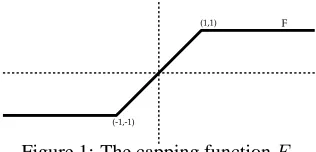
We next introduce an key re-parametrization, defining µ = ν/Z. We also denote by F(·) the capping functionF(x) = max{−1,min{1, x}}. A simple illustration of the capping function is given in Fig. 1. Equipped with these definition we can rewrite (6) as follows,
pj =qj+
1
νF(µuj−νqj) . (7)
Given u,q, andν, the value ofµcan be found by usingPjmjpj =Pjmjqj = 1, which implies
G(ν, µ)=def
n
X
j=1
mjF(µuj−νqj) = 0 . (8)
We defer the derivation of the actual algorithm for computingµ(and in turnp) to the next section. In the meanwhile let us continue to explore the rich
structure of the general solution. Note thatµ,uare interchangeable with ν,q. We can thus swap the roles of the prior distribution with the observed dis-tribution and obtain an analogous characterization. In the next section we further explore the depen-dence of µ on ν. The structure we reveal shortly serves as our infrastructure for deriving efficient al-gorithms for following the regularization path.
4 The functionµ(ν)
In order to explore the dependency ofµonν let us introduce the following sums
M = X
j∈I+ mj −
X
j∈I−
mj
U = X
j∈I0 mjuj
Q = X
j∈I0
mjqj . (9)
Fixingνand using (9), we can rewrite (8) as follows
µU −νQ+M= 0 . (10)
Clearly, so long as the partition of[n]into the sets
I+, I−, I0 is intact, there is a simple linear relation
between µand ν. The number of possible subsets
I−, I0, I+ is finite. Thus, the range 0 < ν < ∞
decomposes into a finite number of intervals each of which corresponds to a fixed partition of[n]into
I+, I−, I0. In each interval µis a linear function of
ν, unlessI0is empty. Letν∞be the smallestνvalue
for whichI0 is empty. Letµ∞be its corresponding
µvalue. IfI0is never empty for any finite value ofν
we defineν∞=µ∞=∞. Clearly, replacing(ν, µ) with (κν, κµ) for any κ ≥ 1 and ν ≥ ν∞ yields the same feasible solution as I+(κν) = I+(ν),
I−(αν) =I−(ν). Hence, as far as the original prob-lem is concerned there is no reason to go pastν∞
during the process of characterizing the solution. We recap our derivation so far in the following lemma.
Lemma 4.1 For 0 ≤ ν ≤ ν∞, the value of µ as defined by (7) is a unique. Further, the functionµ(ν) is a piecewise linear continuous function inν. When
linear sub-intervals the function can attain. To study this property, we take a geometric view of the plane defined by (ν, µ). Our combinatorial characteriza-tion of the number of sub-intervals makes use of the following definitions of lines inR2,
ℓ+j = {(ν, µ)|ujµ−qjν = +1} (11)
ℓ−j = {(ν, µ)|ujµ−qjν =−1} (12)
ℓ0 = {(ν, µ)|µU −νQ+M= 0} ,(13)
where−∞< ν <∞andj ∈[n]. The next theorem gives an upper bound on the number of linear seg-ments the functionµ()may attain. While the bound is quadratic in the dimension, for both artificial data and real data the bound is way too pessimistic.
Theorem 4.2 The piecewise linear function µ(ν) consists of at mostn2 linear segments forν ∈R
+.
Proof Since we showed that that µ(ν) is a piece-wise linear function, it remains to show that it has at most n2 linear segments. Consider the two dimensional function G(ν, µ) from (8). The (ν, µ) plane is divided by the 2n straight lines
ℓ1, ℓ2, . . . , ℓn, ℓ−1, ℓ−2, . . . , ℓ−ninto at most2n2+1
polygons. The latter property is proved by induc-tion. It clearly holds forn= 0. Assume that it holds for n−1. Line ℓn intersects the previous 2n−2
lines at no more than 2n−2points, thus splitting at most 2n−1polygons into two separate polygo-nal parts. Line ℓ−n is parallel to ℓn, again adding
at most2n−1 polygons. Recapping, we obtain at most2(n−1)2 + 1 + 2(2n−1) = 2n2+ 1
poly-gons, as required per induction. Recall thatµ(ν)is linear inside each polygon. The two extreme poly-gons whereG(ν, µ) =±Pnj=1mjclearly disallow
G(ν, µ) = 0, henceµ(ν)can have at most2n2−1 segments for−∞ < ν < ∞. Lastly, we use the symmetry G(−ν,−µ) = −G(ν, µ) which implies that forν ∈R+there are at mostn2segments.
This result stands in contrast to the Lasso homotopy tracking procedure (Osborne et al., 2000), where the worst case number of segments seems to be expo-nential inn. Moreover, when the prioruis uniform,
uj = 1/Pnj=1mj for all j ∈ [n], the number of
segments is at mostn+ 1. We defer the analysis of the uniform case to a later section as the proof stems from the algorithm we describe in the sequel.
0 20 40 60 80 100 0
10 20 30 40 50
ν
[image:4.612.345.512.69.201.2]µ
Figure 2: An illustration of the functionµ(ν)for a syn-thetic3dimensional example.
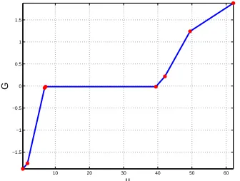
10 20 30 40 50 60 −1.5
−1 −0.5 0 0.5 1 1.5
µ
G
Figure 3: An illustration of the functionG(µ)for a syn-thetic4dimensional example and aν= 17.
5 Algorithm for a Single Relaxation Value
Suppose we are givenu,q,mand a specific relax-ation value ν˜. How can we find p? The obvious approach is to solve the one dimensional monotoni-cally nondecreasing equationG(µ) def=G(˜ν, µ) = 0 by bisection. In this section we present a more effi-cient and direct procedure that is guaranteed to find the optimal solution p in a finite number of steps. Clearly G(µ) is a piecewise linear function with at most 2neasily computable change points of the slope. See also Fig. (5) for an illustration of G(·). In order to find the slope change points we need to calculate the point(ν, µj)for all the linesℓ±jwhere
1≤j≤n. Concretely, these values are
µj =
νq|j|+ sign(j)
u|j| . (14)
We next sort the above values ofµj and denote the
resulting sorted list asµπ1 ≤µπ2 ≤ · · · ≤µπ2n. For
[image:4.612.343.511.255.382.2]in (9), for the line segmentµπj−1 < µ < µπj
(de-noting µπ0 = −∞, µπ2n+1 = ∞). We compute
the sums Mj,Uj,Qj incrementally, starting from
M0 = −Pni=1mi, U0 = Q0 = 0. Once the
values ofj−1’th sums are known, we can compute the next sums in the sequence as follows,
Mj = Mj−1+m|πj|
Uj = Uj−1−sign(πj)m|πj|u|πj|
Qj = Qj−1−sign(πj)m|πj|q|πj| .
From the above sums we can compute the value of the functionG(ν, µ)at the end point of the line seg-ment (µπj−1, µπj), which is the same as the start
point of the line segment(µπj, µπj+1),
Gj = Mj−1+Uj−1µj− Qj−1ν
= Mj +Ujµj − Qjν .
The optimal value ofµresides in the line segment for whichG(·)attains0. Such a segment must exist since G0 = M0 = −Pni=1mi < 0 and G2n =
−M0 > 0. Therefore, there exists an index 1 ≤
j <2n, whereGj ≤0≤Gj+1. Once we bracketed
the feasible segment forµ, the optimal value ofµis found by solving the linear equation (10),
µ= (Qjν − Mj) /Uj . (15)
From the optimal value ofµit is straightforward to constructpusing (7). Due to the sorting step, the al-gorithm’s run time isO(nlog(n))and it takes linear space. The number of operations can be reduced to
O(n)using a randomized search procedure.
6 Homotopy Tracking
We now shift gears and focus on the main thrust of this paper, namely, an efficient characterization of the entire regularization path for the maximum entropy problem. Since we have shown that the optimal solution p can be straightforwardly ob-tained from the variable µ, it suffices to efficiently track the function µ(ν) as we traverse the plane (ν, µ) from ν = 0 through the last change point which we denoted as (ν∞, µ∞). In this section we give an algorithm that traverses µ(ν) by lo-cating the intersections of ℓ0 with the fixed lines
ℓ−n, ℓ−n+1, . . . , ℓ−1, ℓ1, . . . , ℓn and updatingℓ0
af-ter each inaf-tersection.
More formally, the local homotopy tracking fol-lows the piecewise linear functionµ(ν), segment by segment. Each segment corresponds to a subset of the lineℓ0for a given triplet(M,U,Q). It is simple
to show thatµ(0) = 0, hence we start with
ν = 0, M= 0, U =Q= 1 . (16)
We now track the value ofµasνincreases, and the relaxation parameter1/ν decreases. The character-ization ofℓ0 remains intact until ℓ0 hits one of the
linesℓj for1 ≤ |j| ≤ n. To find the line
intersect-ingℓ0we need to compute the potential intersection
points(νj, µj) =ℓ0∩ℓjwhich amounts to
calculat-ingν−n, ν−n+1, . . . , ν−1, ν1, ν2,· · ·, νnwhere
νj = M
u|j|+Usign(j)
Qu|j|− Uq|j| . (17)
The lines for which the denominator is zero cor-respond to infeasible intersection and can be dis-carded. The smallest value νj which is larger than
the current traced value ofνcorresponds to the next line intersectingℓ0.
While the above description is mathematically sound, we devised an equivalent intersection in-spection scheme which is more numerically stable and efficient. We keep track of partition I−, I0, I1
through the vector,
sj =
−1 j∈I−
0 j∈I0
+1 j∈I+
.
Initially s1 = s2 = · · · = sn = 0. What kind of
intersection doesℓ0 have with ℓj? Recall that QU is
the slope ofℓ0 while uq|j|
|j| is the slope of ℓj. Thus
Q
U >
q|j|
u|j| means that the|j|’th constraint is moving
“up” fromI−toI0or fromI0toI+. WhenQU < uq|j| |j|
the|j|’th constraint is moving “down” fromI+toI0
or fromI0 toI−. See also Fig. 4 for an illustration
of the possible transitions between the sets. For in-stance, the slope ofµ(ν) on the bottom left part of the figure is larger than the slope the line it inter-sects. Since this line defines the boundary between
I− and I0, we transition from I− to I0. We need
only consider 1 ≤ |j| ≤ nof the following types. Moving “up” fromI−toI0requires
Figure 4: Illustration of the possible intersections be-tweenµ(ν)andℓj and the corresponding transition
be-tween the setsI±, I0.
Similarly, moving “down” fromI+toI0requires
s|j|= 1 j >0 Qu|j|− Uq|j|<0 .
Finally, moving “up” or “down” fromI0entails
s|j|= 0 j(Qu|j|− Uq|j|)>0 .
If there are no eligibleνj’s, we have finished
travers-ing µ(). Otherwise let index j belong to the the smallest eligible νj. Infinite accuracy guarantees
thatνj ≥ν. In practice we perform the update
ν ← max(ν, νj)
M ← M+ sign(Qu|j|− Uq|j|)m|j| U ← U+ 2s|j|−1 m|j|u|j| Q ← Q+ 2s|j|−1 m|j|q|j| sj ← sj+ sign(Qu|j|− Uq|j|) .
We are done with the tracking process when I0 is
empty, i.e. for allj sj 6= 0.
The local homotopy algorithm takes O(n) mem-ory andO(nk)operations wherekis the number of change points in the function µ(ν). This algorithm is simple to implement, and when k is relatively small it is efficient. An illustration of the tracking result,µ(ν), along with the linesℓ±j, that provide a
geometrical description of the problem, is given in Fig. 5.
7 Uniform Prior
We chose to denote the prior distribution asuto un-derscore the fact that in the case of no prior
knowl-0 0.2 0.4 0.6 0.8 1 1.2 1.4 1.6 1.8
−4 −2 0 2 4 6 8 10
ν
µ
Figure 5: The result of the homotopy tracking for a4
dimensional problem. The linesℓjforj <0are drawn in
blue and forj >0in red. The functionµ(ν)is drawn in green and its change points in black. Note that although the dimension is4the number of change points is rather small and does not exceed4either in this simple example.
edgeuis the uniform distribution,
u=def uj = n
X
i=1
mi
!−1
.
In this case the objective function amounts to the negative entropy and by flipping the sign of the ob-jective we obtain the classical maximum entropy problem. The fact that the prior probability is the same for all possible observations infuses the prob-lem with further structure which we show how to exploit in this section. Needless to say though that all the results we obtained thus far are still valid.
Let us consider a point(ν, µ)on the boundary be-tweenI0 andI+, namely, there exist a lineℓ+isuch
that,
µui−νqi =µu−νqi= 1 .
By definition, for anyj∈I0 we have
µuj −νqj =µu−νqj <1 =µu−νqi .
Thus,qi < qj for allj ∈I0which implies that
mjuqj > mjuqi . (18)
Summing overj∈I0we get that
Qu = X
j∈I0
mjqju >
X
j∈I0
mjuqi = Uqi ,
hence,
qi
ui
= qi u <
[image:6.612.80.290.71.213.2]and we must be moving “up” fromI0toI+when the
lineℓ0hitsℓi. Similarly we must be moving “down”
from whenℓ0 hits on the boundary betweenI0 and
I−. We summarize these properties in the following theorem.
Theorem 7.1 When the prior distribution uis uni-form, I−(ν) and I+(ν) are monotonically
nonde-creasing and I0(ν)is monotonically nonincreasing
in ν > 0 . Further, the piecewise linear function
µ(ν)consists of at mostn+ 1line segments. The homotopy tracking procedure when the prior is uniform is particularly simple and efficient. In-tuitively, there is a sole condition which controls the order in which indices would enterI± fromI0,
which is simply how “far” eachqiis fromu, the
sin-gle prior value. Therefore, the algorithm starts by sorting q. Let qπ1 > qπ2 > · · · > qπn denote the
sorted vector. Instead of maintaining the vector of set indicatorss, we merely maintain two indicesj−
and j+ which designate the size ofI− and I+ that
were constructed thus far. Due to the monotonic-ity property of the setsI± asν grows, the two sets can be written as, I− = {πj|1 ≤ j < j−} and
I+ = {πj|j+ < j ≤ n}. The homotopy
track-ing procedure starts as before withν = 0,M= 0,
U =Q= 1. We also setj− = 1andj+ =nwhich
by definition imply thatI±are empty andI0 = [n].
In each tracking iteration we need to compare only two values which we compactly denote as,
ν±= Mu ± U
Qu − Uqπj±
.
When ν− ≤ ν+ we just encountered a transition
from I0 toI− and as we encroach I− we perform
the updates, ν ← ν−, M ← M − mπj−, U ←
U −mπj−u, Q ← Q −mπj−qπj−, j−←j−+ 1.
Similarly when ν− > ν+ we perform the updates
ν ←ν+, M ← M + mπj+, U ← U − mπj+u,
Q ← Q − mπj+qπj+, j+ ←j+ − 1.
The tracking process stops whenj− > j+ as we
exhausted the transitions out of the setI0which
be-comes empty. Homotopy tracking for a uniform prior takes O(n) memory and O(nlog(n)) opera-tions and is very simple to implement.
We also devised a global homotopy tracking algo-rithms that requires a priority queue which facilitates insertions, deletions, and finding the largest element
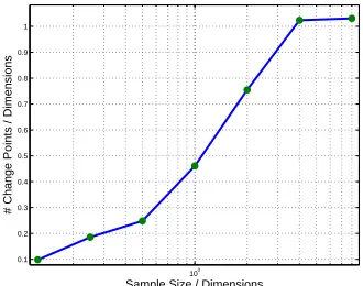
100
0.1 0.2 0.3 0.4 0.5 0.6 0.7 0.8 0.9 1
Sample Size / Dimensions
[image:7.612.342.507.76.206.2]# Change Points / Dimensions
Figure 6: The number of line-segments in the homotopy as a function of the number of samples used to build the observed distributionq.
in the queue in O(log(n))time. The algorithm re-quiresO(n)memory and O(n2log(n))operations.
Clearly, if the number of line segments constituting
µ(ν) is greater than nlog(n) (recall that the upper bound is O(n2)) then the global homotopy proce-dure is faster than the local one. However, as we show in Sec. 8, in practice the number of line seg-ments is merely linear and it thus suffices to use the local homotopy tracking algorithm.
8 Number of line segments in practice
The focus of the paper is the design and analysis of a novel homotopy method for maximum entropy problems. We thus left with relatively little space to discuss the empirical aspects of our approach. In this section we focus on one particular experimental facet that underscores the usability of our apparatus. We briefly discuss current natural language applica-tions that we currently work on in the next section.
The practicality of our approach hinges on the number of line segments that occur in practice. Our bounds indicate that this number can scale quadrat-ically with the dimension, which would render the homotopy algorithm impractical when the size of the alphabet is larger than a few thousands. We there-fore extensively tested the actual number of line seg-ments in the resulting homotopy whenuandq are Zipf (1949) distributions. We used an alphabet of size50,000 in our experiments. The distribution u
was set to be the Zipf distribution with an offset pa-rameter of 2, that is, ui ∼ 1/(i+ 2). We defined
a plain Zipf distribution without an offset, namely ¯
qi ∼ 1/i. We then sampledn/2l letters according
to the distribution q¯wherel ∈ −3, . . . ,3. Thus the smallest sample wasn/23 = 6,250and the largest sample wasn/3−3 = 40,000. Based on the sample
we defined the observed distribution q such thatqi
is proportional to the number of times the i’th let-ter appeared in the sample. We repeated the process 100 times for each sample size and report average results. Note that when the sample is substantially smaller than the dimension the observed distribution
q tends to be “simple” as it consists of many zero components. In Fig. 6 we depict the average num-ber line segments for each sample size. When the sample size is one eighth of the dimension we aver-age st most0.1nline segments. More importantly, even when the size of the sample is fairly large, the number of lines segments is linear in the dimension with a constant close to one. We also performed experiments with large sample sizes for which the empirical distribution q is very close to the mother distribution q¯. We seldom found that the number of line segments exceeds 4n and the mode is around 2n. These findings render our approach usable even in the very large natural language applications.
9 Conclusions
We presented a novel efficient apparatus for tracking the entire relaxation path of maximum entropy prob-lems. We currently study natural language process-ing applications. In particular, we are in the process of devising homotopy methods for domain adapta-tion Blitzer (2008) and language modeling based on context tree weighting (Willems et al., 1995). We also examine generalization of our approach in which the relative entropy objective is replaced with a separable Bregman (Censor and Zenios, 1997) function. Such a generalization is likely to distill further connections to the other homotopy methods, in particular the least angle regression algorithm of Efron et al. (2004) and homotopy methods for the Lasso in general (Osborne et al., 2000). We also plan to study separable Bregman functions in order to de-rive entire path solutions for less explored objectives such as the Itakura-Saito spectral distance (Rabiner and Juang, 1993) and distances especially suited for natural language processing.
References
A.L. Berger, S.A. Della Pietra, and V. J. Della Pietra. A maximum entropy approach to natural lan-guage processing. Computational Linguistics, 22 (1):39–71, 1996.
John Blitzer. Domain Adaptation of Natural Lan-guage Processing Systems. PhD thesis, University of Pennsylvania, 2008.
S. Boyd and L. Vandenberghe. Convex Optimiza-tion. Cambridge University Press, 2004.
Y. Censor and S.A. Zenios. Parallel Optimization: Theory, Algorithms, and Applications. Oxford University Press, New York, NY, USA, 1997.
S. Della Pietra, V. Della Pietra, and J. Lafferty. In-ducing features of random fields. IEEE Trans-actions on Pattern Analysis and Machine Intelli-gence, 5:179–190, 1997.
M. Dud´ık, S. J. Phillips, and R. E. Schapire. Maxi-mum entropy density estimation with generalized regularization and an application to species distri-bution modeling. Journal of Machine Learning Research, 8:1217–1260, June 2007.
Bradley Efron, Trevor Hastie, Iain Johnstone, and Robert Tibshirani. Least angle regression. Annals of Statistics, 32(2):407–499, 2004.
Edwin T. Jaynes. Prior probabilities. IEEE Transac-tions on Systems Science and Cybernetics, SSC-4 (3):227–241, September 1968.
Michael R. Osborne, Brett Presnell, and Berwin A. Turlach. On the lasso and its dual. Journal of Computational and Graphical Statistics, 9(2): 319–337, 2000.
L. Rabiner and B.H. Juang. Fundamentals of Speech Recognition. Prentice Hall, 1993.
F. M. J. Willems, Y. M. Shtarkov, and T. J. Tjalkens. The context tree weighting method: basic proper-ties. IEEE Transactions on Information Theory, 41(3):653–664, 1995.