Abstract—This paper presents the identification of the topological spatial relations that can exist between a Circular Spatially Extended Point and a Line in the geographical space. For the identification of the topological spatial relations that can exist between these two types of objects, the intersections existing between the several parts of the objects were verified. Using 14 conditions and the respective proofs, a set of 38 topological spatial relations were identified. The geometric characterization of the topological relations was also achieved, proving the existence of such relations.
Index Terms—Qualitative reasoning, Spatially Extended Point, Spatial Reasoning, Topological spatial relations.
I. INTRODUCTION
Spatial relations between objects have been classified into several types [1, 2], including direction relations [3],
distance relations [4] and topological relations [5]. Topological relations are those spatial relations preserved under continuous transformations of the space, such as rotation or scaling.
Research on topological spatial relations between different types of objects (points, lines and regions) has been undertaken for many years, identifying the topological spatial relations between regions, lines, regions and lines, regions and points, among others, and representing their geometric realization, proving the existence of such relations. Some of the works undertaken so far include the identification of the topological spatial relations between regions [6], between lines [6], between regions and lines [6, 7], between regions with broad boundaries [8], between a spatially extended point and a region [9], between broad lines [10], and between lines with broad boundaries [10], only to mention a few.
The relevance of the identification of such topological spatial relations is associated with the need to conceptualize the spatial relations that can exist among several objects in the geographical space. The obtained models can be used as a computational framework for spatial reasoning. Their implementation in a system, like a Geographical Information System, allows the representation and manipulation of complex objects associated with complex realities.
The work described in this paper is associated with the
Manuscript received March 23, 2008.
M. Y. Santos is with the Information Systems Department, University of Minho, Campus de Azurém, 4800-058 Guimarães, Portugal (corresponding author, phone: +351-253-510308; fax: +351-253-510300; e-mail: maribel@ dsi.uminho.pt).
A. Moreira is with the Information Systems Department, University of Minho, Campus de Azurém, 4800-058 Guimarães, Portugal (e-mail: [email protected]).
topological spatial relations existing between a Circular Spatially Extended Point and a Line. A Circular Spatially Extended Point is a region-like object characterized by the inclusion of a point and a region that defines the area of influence of that point. In the scope of this work, the Circular Spatially Extended Point represents a complex object in the sense that the point and its region of influence are not dissociable. The identification of the topological spatial relations between a Circular Spatially Extended Point and a Line was first addressed by the authors of this paper in [11] to use them in the prediction of mobile users’ future positions in a context-aware mobile environment. In this paper this work is revisited and all formal proofs are provided demonstrating the validity of the work undertaken.
Looking at the abstractions usually used to represent spatial objects, single points, single lines and single regions, and their complex data types, complex points, complex lines and complex regions, and for whom the topological spatial relations existing between them were already identified [12], none of these abstractions allows the representation of the particular integration of a point and a region, here identified as a Circular Spatially Extended Point. For regions with broad boundaries, the two regions that integrate the object “region with broad boundary” are 2-dimensional components, also not representing the 0-dimensional part of a Circular Spatially Extended Point (its pivot) [13].
The following sections are organized as follows. Section 2 is dedicated to an overview of the principles behind qualitative spatial reasoning. Section 3: i) describes the conceptual framework adopted for the identification of the topological spatial relations that can exist between a Circular Spatially Extended Point and a Line; ii) presents the formal proofs for all the adopted conditions; and iii) shows the geometrical characterization of the identified topological relations. Section 4 concludes with some remarks about the work undertaken.
II. QUALITATIVE SPATIAL REASONING
Human beings use qualitative identifiers extensively to simplify reality and to perform spatial reasoning more efficiently. Spatial reasoning is the process by which information about objects in space and their relationships are gathered through measurement, observation or inference and used to arrive at valid conclusions regarding the relationships of the objects [14]. Qualitative spatial reasoning [15] is based on the manipulation of qualitative spatial relations, for which composition tables facilitate reasoning [14, 16], thereby allowing the inference of new spatial knowledge.
Spatial relations include direction relations, distance
How a Circular Spatially Extended Point is
Topological Related with a Line?
relations and topological relations.
A. Direction Spatial Relations
Direction relations describe where objects are placed relative to each other. Three elements are needed to establish an orientation: two objects and a fixed point of reference (usually the North Pole) [1, 3]. Cardinal directions can be expressed using numerical values specifying degrees (0º,
45º…) or using qualitative values or symbols, such as North
or South, which have an associated acceptance region. The
regions of acceptance for qualitative directions can be obtained by projections (also known as half-planes) or by cone-shaped regions (Fig. 1).
NW NE
SE SW
N
E
[image:2.595.332.515.60.173.2]S W
Fig. 1 – Direction relations by projection and cone-shaped systems
B. Distance Spatial Relations
Distances are quantitative values determined through measurements or calculated from known co-ordinates of two objects in some reference system. The frequently used definition of distance can be achieved using the Euclidean geometry and Cartesian coordinates. In a two-dimensional Cartesian system, it corresponds to the length of the shortest possible path (a straight line) between two objects, which is also known as the Euclidean distance [16]. Usually a metric quantity is mapped onto some qualitative indicator such as
very close or far for human common-sense reasoning [4].
Qualitative distances must correspond to a range of quantitative values specified by an interval. The adoption of the qualitative distances very close(vc), close(c), far(f) and
veryfar(vf), intuitively describe distances from the nearest to the furthest. An order relationship exists among these relations, where a lower order (vc) relates to shorter quantitative distances and a higher order (vf) relates to longer quantitative distances [16] (Fig. 2).
[image:2.595.78.264.217.281.2]vf f c vc
Fig. 2 – Qualitative distances
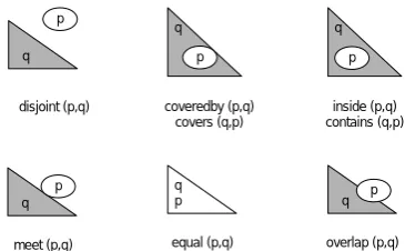
C. Topological Spatial Relations
Topological relations are those relationships that are invariant under continuous transformations of space such as rotation or scaling. There are eight topological relations that can exist between two planar regions without holes: disjoint,
contains, inside, equal, meet, covers, covered by and overlap (Fig. 3). These relations can be defined considering the intersections between the two regions, their boundaries and their complements [5].
overlap (p,q) equal (p,q)
meet (p,q)
q p
q p q
p
disjoint (p,q) coveredby (p,q) covers (q,p)
inside (p,q) contains (q,p)
q
p q
p q p
Fig. 3 – Topological spatial relations III. TOPOLOGICAL SPATIAL RELATIONS BETWEEN A
CIRCULAR SPATIALLY EXTENDED POINT AND A LINE
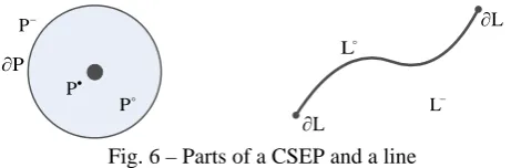
A Circular Spatially Extended Point (CSEP) can be considered as a region-like concept. A CSEP (Fig. 4) has its own interior, boundary and exterior. While it shares the same concepts of interior, boundary and exterior of a region, the CSEP is distinguished from a general region by the identification of a point within the interior called the pivot. The pivot is conceptually similar to a 0-dimension object. A major difference between a usual point and a pivot is that a pivot has an area of influence that defines the boundary of the CSEP [9].
Pivot
Fig. 4 – A circular spatially extended point
From a geometrical point of view, a simple line, representing a linear curve, has a boundary with two simple points, each of which has no extension [6, 12] (Fig. 5). The definition of a simple line usually refers to a 1-dimensional object of ℜ2 with no self-intersections [17]. Closed lines are lines without end-points [17], so they lay out of the definition of simple line and consequently are not considered in the scope of the work presented in this paper.
Fig. 5 – A simple line
[image:2.595.107.226.563.667.2]P ∂
P
•
P
−
P
L ∂
L ∂
−
[image:3.595.50.281.52.128.2]L L
Fig. 6 – Parts of a CSEP and a line
Each relation (R) between a CSEP (P) and a line (L) is characterized by 12 (4x3) intersections with empty (∅) or non-empty (¬∅) values depending on how the geographical objects are related (Equation 1).
⎥ ⎥ ⎥ ⎥ ⎥
⎦ ⎤
⎢ ⎢ ⎢ ⎢ ⎢
⎣ ⎡
∂ ∂ ∂ ∂ ∂
∂ ∂
=
− − −
−
− − − • •
•
L P L P L P
L P L P L P
L P L P L P
L P L P L P
) , (
∩ ∩
∩
∩ ∩
∩
∩ ∩
∩
∩ ∩
∩
L P
R (1)
The several conditions proposed by Egenhofer and Herring [6] for the identification of the topological relations between regions, lines and points in a Geographic Database were analyzed. Following these authors’ suggestions, 9 conditions were adopted and adapted to the specific context of this work. These conditions are associated with the definition of the topological spatial relations that can exist between regions, between a region and a line, and between a non-point object (a region or a line) and a point, and are here described as conditions 1 to 9. Additional conditions were defined attending to the particular case of the definition of the topological relations between a CSEP and a line. These conditions are referred as condition 10 to condition 14. The whole set of conditions and their formal proofs are described as follows:
Condition 1. The exteriors of the two objects (P and L) intersect with each other (Equation 2).
⎥ ⎥ ⎥ ⎥
⎦ ⎤
⎢ ⎢ ⎢ ⎢
⎣ ⎡
− −
− − −
− − −
− − −
≠
φ )
, (P L
R (2)
Proof: Knowing that P•∪ P°∪∂P ∪ P- = ℜ2 and that L°∪
∂L ∪ L- = ℜ2, the statement P-∩ L- = ∅ can only be possible either if: i) P•∪ P°∪∂P = ℜ2; ii) L°∪∂L = ℜ2; or iii) P•∪ P°
∪∂P ∪ L° ∪∂L = ℜ2. However, all these conditions are impossible since the objects P, L and P ∪ L are bounded and
ℜ2
is unbounded.
Condition 2. If P’s boundary intersects L’s exterior then P’s interior must intersect L’s exterior as well, and vice-versa
(Equation 3 where ∨ means or).
⎥ ⎥ ⎥ ⎥
⎦ ⎤
⎢ ⎢ ⎢ ⎢
⎣ ⎡
− ¬
− − −
− − −
− − −
∨ ⎥ ⎥ ⎥ ⎥
⎦ ⎤
⎢ ⎢ ⎢ ⎢
⎣ ⎡
− − −
¬ − −
− −
− − −
≠
φ φ φ φ )
, (P L
R (3)
Proof: Assuming that the constraint rules are false, then ∂P
∩ L- = ¬∅⇒ P°∩ L- = ∅ and ∂L ∩ P- = ¬∅⇒ L°∩ P- = ∅. Knowing that L°∪∂L ∪ L- = ℜ2, this leads to P°∩ (L°∪∂L
∪ L-) = P°∩ℜ2 = ∅, which is a contradiction to the assumed non-emptiness of the interior of a CSEP, here represented by a region, so P°∩ℜ2 = ¬∅. For the other rule, and knowing that P•∪ P°∪∂P ∪ P- = ℜ2, this leads to L°∩ (P•∪ P°∪∂P
∪ P-) = L°∩ℜ2 = ∅, which is a contradiction to the assumed non-emptiness of the interior of a line, so L°∩ℜ2 = ¬∅.
Condition 3. P’s boundary intersects with at least one part of L and vice-versa (Equation 4).
⎥ ⎥ ⎥ ⎥
⎦ ⎤
⎢ ⎢ ⎢ ⎢
⎣ ⎡
− −
− −
− −
− − −
∨ ⎥ ⎥ ⎥ ⎥
⎦ ⎤
⎢ ⎢ ⎢ ⎢
⎣ ⎡
− − −
− − −
− − −
≠
φ φ φ φ
φ φ ) , (P L
R (4)
Proof: Knowing that P•∪ P°∪∂P ∪ P- = ℜ2, L°∪∂L ∪ L -= ℜ2, and that only non-empty parts of both objects are considered, it is obtained that ∂P ∩ℜ2 = ¬∅ and that ∂L ∩
ℜ2
= ¬∅. These statements are equivalent to ∂P ∩ (L°∪∂L
∪ L-) = ¬∅ and ∂L ∩ (P•∪ P° ∪∂P ∪ P-) = ¬∅, which verify the constrain rules expressed in equation 4.
Condition 4. If both interiors are disjoint then P’s interior cannot intersect with L’s boundary (Equation 5).
⎥ ⎥ ⎥ ⎥
⎦ ⎤
⎢ ⎢ ⎢ ⎢
⎣ ⎡
− − −
− − −
− ¬
− − −
≠ φ φ
) , (P L
R (5)
Proof: Assuming that both interiors are disjoint, Pº ∩ Lº =
∅, and that P’s interior intersects L’s boundary, Pº ∩∂L =
¬∅, the concept of simple line is not accomplished since the two end points that represent the boundary of the line are contiguous to the points that integrate the interior of the line and cannot be disaggregated from them. So, it is impossible for a line to be disjoint from the interior of a region and at the same time its boundary be intersected by the interior of the region.
Condition 5. If L’s interior intersects with P’s interior and exterior, then it must also intersect with P’s boundary (Equation 6).
⎥ ⎥ ⎥ ⎥
⎦ ⎤
⎢ ⎢ ⎢ ⎢
⎣ ⎡
− − ¬
− −
− − ¬
− − −
≠
φ φ
φ ) , (P L
R (6)
boundary).
Condition 6. P’s interior always intersects with L’s exterior (Equation 7).
⎥ ⎥ ⎥ ⎥
⎦ ⎤
⎢ ⎢ ⎢ ⎢
⎣ ⎡
− − −
− − −
− −
− − −
≠ φ
) , (P L
R (7)
Proof: Let’s assume that the condition is wrong, then Pº ∩ L- = ∅. To confirm this condition, the statement Pº = Lº ∪∂L, or the statement Pº = Lº, must be verified. Since P is a region-like object (2-dimensional) and L represents a simple line object (1-dimensional) this leads to an impossible situation since they cannot be equal.
Condition 7. P’s boundary always intersects with L’s exterior (Equation 8).
⎥ ⎥ ⎥ ⎥
⎦ ⎤
⎢ ⎢ ⎢ ⎢
⎣ ⎡
− − −
− −
− − −
− − −
≠ φ
) , (P L
R (8)
Proof: Let’s assume that the condition is wrong, then ∂P ∩ L- = ∅. To confirm this condition, the statement ∂P = ∂L ∪ Lº must be verified. Since a simple line has two end-points, a non-empty boundary, and the boundary of a region is a closed line with no end-points, the statement is not verified since the boundary of a region is not equal (in conceptual terms) to a simple line.
Condition 8. L’s interior must intersect with at least one of the four parts of P (Equation 9).
⎥ ⎥ ⎥ ⎥
⎦ ⎤
⎢ ⎢ ⎢ ⎢
⎣ ⎡
− −
− −
− −
− −
≠
φ φ φ φ
) , (P L
R (9)
Proof: Knowing that P•∪ P°∪∂P ∪ P- = ℜ2, L°∪∂L ∪ L -= ℜ2, and that only non-empty parts of objects are considered, it is possible to say that Lº ∩ℜ2 = ¬∅. These statements are equivalent to Lº ∩ (P•∪ P°∪∂P ∪ P-) = ¬∅, which verifies the constrain rules expressed in equation 9.
Condition 9. P’s pivot can only intersect with a single part of L (Equation 10).
⎥ ⎥ ⎥ ⎥
⎦ ⎤
⎢ ⎢ ⎢ ⎢
⎣ ⎡
− − −
− − −
− − −
¬ − ¬
∨ ⎥ ⎥ ⎥ ⎥
⎦ ⎤
⎢ ⎢ ⎢ ⎢
⎣ ⎡
− − −
− − −
− − −
¬ ¬ −
∨ ⎥ ⎥ ⎥ ⎥
⎦ ⎤
⎢ ⎢ ⎢ ⎢
⎣ ⎡
− − −
− − −
− − −
− ¬ ¬
≠
φ φ φ φ φ
φ
) , (P L
R (10)
Proof: Since P• is 0-dimensional geometric primitive, representing a position, and by definition it has no boundary
(a simple point can be specified as having the following characteristics: ∂P = ∅ and P° = P ([12]), it that can only be intersected by one of the three parts considered for a line, L°,
∂L or L-. This leads to the conditions P•∩ L° = ¬∅∨ P•∩∂L = ¬∅∨ P•∩ L- = ¬∅.
Condition 10. P’s pivot must intersect with at least one part of L (Equation 11).
⎥ ⎥ ⎥ ⎥
⎦ ⎤
⎢ ⎢ ⎢ ⎢
⎣ ⎡
− − −
− − −
− − − ≠
φ φ φ
) , (PL
R (11)
Proof: Knowing that P•∪ P°∪∂P ∪ P- = ℜ2, L°∪∂L ∪ L -= ℜ2, and that only non-empty parts of objects are considered, it is possible to say that P•∩ℜ2 = ¬∅. These statements are equivalent to P• ∩ (L° ∪ ∂L ∪ L-) = ¬∅, which verifies the constrain rules expressed in equation 11.
Condition 11. If P’s interior intersects with L’s interior, and P’s exterior intersects with L’s boundary, then the P’s boundary must intersect with L’s interior (Equation 12).
⎥ ⎥ ⎥ ⎥
⎦ ⎤
⎢ ⎢ ⎢ ⎢
⎣ ⎡
− ¬ −
− −
− − ¬
− − −
≠
φ φ
φ ) , (PL
R (12)
Proof: As a simple line integrates two end points that represent the boundary of the line and that are contiguous to the connected set of points that integrate the interior of the line, it is impossible the intersection of L’s interior with P’s interior and the intersection of L’s boundary with P’s exterior, without L’s interior also intersecting P’s boundary (between P’s interior and exterior we have P’s boundary).
Condition 12. The boundary of a simple line L (simple lines are one-dimensional, continuous features embedded in the plane [12]) can only intersect with at most two parts of P (Equation 13).
⎥ ⎥ ⎥ ⎥
⎦ ⎤
⎢ ⎢ ⎢ ⎢
⎣ ⎡
− ¬ −
− − −
− ¬ −
− ¬ −
∨ ⎥ ⎥ ⎥ ⎥
⎦ ⎤
⎢ ⎢ ⎢ ⎢
⎣ ⎡
− ¬ −
− ¬ −
− − −
− ¬ −
∨ ⎥ ⎥ ⎥ ⎥
⎦ ⎤
⎢ ⎢ ⎢ ⎢
⎣ ⎡
− ¬ −
− ¬ −
− ¬ −
− − −
∨ ⎥ ⎥ ⎥ ⎥
⎦ ⎤
⎢ ⎢ ⎢ ⎢
⎣ ⎡
− − −
− ¬ −
− ¬ −
− ¬ −
≠
φ φ φ
φ φ φ
φ φ φ φ
φ φ
) , (PL R
(13)
Proof: A simple line has a boundary that integrates two points, each one of them being a 0-dimensional geometric primitive. These two points can only intersect, each of them, one part of the CSEP P. This leads to the intersection of the boundary of L (∂L) with at most two parts of P since the two points of ∂L can intersect the same part of P, with exception to the pivot of P (P•) that can only be intersected by one of the two points of ∂L.
⎥ ⎥ ⎥ ⎥
⎦ ⎤
⎢ ⎢ ⎢ ⎢
⎣ ⎡
− − −
− − −
− −
− ¬ −
≠ φ φ
) , (P L
R (14)
Proof: Assuming that the constraint rule is false, then ∂L ∩ P• = ¬∅⇒ P°∩ L° = ∅. Knowing that L°∪∂L ∪ L- = ℜ2, this leads to P°∩ (L°∪∂L ∪ L-) = P°∩ℜ2 = ∅, which is a contradiction to the assumed non-emptiness of the interior of a CSEP, here represented by a region, so P°∩ℜ2 = ¬∅.
Condition 14. If L’s interior intersects P’s pivot, then P’s interior must intersect L’s interior (Equation 15).
⎥ ⎥ ⎥ ⎥
⎦ ⎤
⎢ ⎢ ⎢ ⎢
⎣ ⎡
− − −
− − −
− −
− − ¬
≠ φ
φ
) , (P L
R (15)
Proof: Assuming that the constraint rule is false, then L°∩ P• = ¬∅⇒ P°∩ L° = ∅. Knowing that L°∪∂L ∪ L- = ℜ2, this leads to P°∩ (L°∪∂L ∪ L-) = P°∩ℜ2 = ∅, which is a contradiction to the assumed non-emptiness of the interior of a CSEP, here represented by a region, so P°∩ℜ2 = ¬∅.
The adoption of a 4x3 matrix for the definition of the intersections between the pivot (P•), interior (P°), boundary (∂P) and exterior (P-) of P, and the interior (L°), boundary (∂L) and exterior (L-) of L, results in the identification of 4096 (212) different matrices. In this set, with a very large number of possible combinations, only a reduced number of matrices represent valid topological relations for the objects in analysis.
In order to support the process of generation of the 4096 different matrices and the elimination of the invalid ones, a computational approach was followed using Mathematica® [18]. This implementation allowed the identification of the 4096 matrices, the definition of the several conditions (Conditions 1 to 14) and the automatic elimination of the invalid patterns associated with those conditions (Equations 2 to 15).
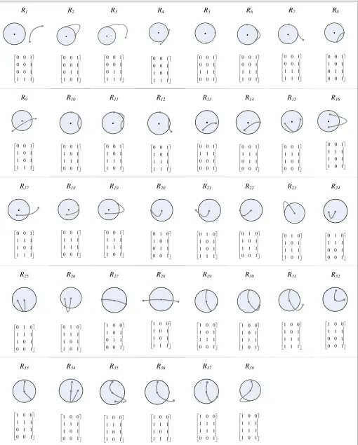
After the application of the 14 conditions, 38 matrices were left as possible ones. Each one of these matrices was manually analyzed to certify their validity. As all the matrices were considered valid, no more conditions were defined. This analysis was undertaken through the geometric realization of the 38 different topological spatial relations, validating the relations in terms of their existence.
Table I (Annex I) presents the identified topological spatial relations (with their geometric realization) and their corresponding matrices. In those matrices the absence of intersection is represented by 0 (∅) and its presence by 1 (¬∅).
IV. CONCLUSION
This paper presented the topological spatial relations that can exist between a CSEP and a line. After the identification
of the conditions that must be verified between the several parts of a CSEP and a line, 38 topological spatial relations were identified. Those relations can now be used in the identification of the composition tables or the conceptual neighborhood graphs that allow spatial reasoning with these two types of objects.
ACKNOWLEDGMENT
We thank Professor Filomena Louro for her revision of the English writing of this paper.
REFERENCES
[1] Frank, A.U., “Qualitative Spatial Reasoning: cardinal directions as an example”. International Journal of Geographical Information Systems, 1996. 10(3): p. 269-290.
[2] Papadias, D. and T. Sellis, “On the Qualitative Representation of Spatial Knowledge in 2D Space”. Very Large Databases Journal, Special Issue on Spatial Databases, 1994. 3(4): p. 479-516.
[3] Freksa, C., “Using Orientation Information for Qualitative Spatial Reasoning”, in Theories and Methods of Spatio-Temporal Reasoning
in Geographic space, A.U. Frank, I. Campari, and U. Formentini,
Editors. 1992, Springer-Verlag: Berlin.
[4] Hernández, D., E. Clementini, and P.D. Felice, Qualitative Distances.
in Spatial Information Theory - A Theoretical Basis for GIS,
Proceedings of the International Conference COSIT'95, 1995. Semmering, Austria: Springer-Verlag.
[5] Egenhofer, M.J., “Deriving the Composition of Binary Topological Relations”. Journal of Visual Languages and Computing, 1994. 5(2): p. 133-149.
[6] Egenhofer, M.J. and J.R. Herring, Categorizing Binary Topological Relations Between Regions, Lines, and Points in Geographic
Databases. Technical Report, 1991, Department of Surveying
Engineering, University of Maine: Orono, USA.
[7] Egenhofer, M.J. and D.M. Mark, “Modeling Conceptual Neighborhoods of Topological Line-Region Relations”. International
Journal of Geographical Information Systems, 1995. 9(5): p. 555-565.
[8] Clementini, E. and P.D. Felice, “Approximate Topological Relations”.
International Journal of Approximate Reasoning, 1997(16): p.
173-204.
[9] Lee, B. and D.M. Flewelling, Spatial Organicism: Relations between a
Region and a Spatially Extended Point. In GIScience 2004 - Third
International Conference on Geographic Information Science. 2004. University of Maryland, USA.
[10] Reis, R., M. Egenhofer, and J. Matos, Topological relations using two
models of uncertainty for lines. In 7th International Symposium on
Spatial Data Accuracy Assessment in Natural Resources and Environment Sciences. 2006. Lisbon, Portugal.
[11] Santos, M.Y. and A. Moreira, Topological Spatial Relations between a
Spatially Extended Point and a Line for Predicting Movement in Space.
In Proceedings of the 10th AGILE Conference on Geographic Information Science. 2007. Aalborg, Denmark.
[12] Schneider, M. and T. Behr, “Topological Relationships Between Complex Spatial Objects”. ACM Transactions on Database Systems, 2006. 31(1): p. 39-81.
[13] Clementini, E. and P.D. Felice, “A spatial model for complex objects with a broad boundary supporting queries on uncertain data”. Data &
Knowledge Engineering, 2001. 37(3): p. 285-305.
[14] Sharma, J., Integrated Spatial Reasoning in Geographic Information
Systems: Combining Topology and Direction, PhD thesis, 1996,
University of Maine.
[15] Abdelmoty, A.I. and B.A. El-Geresy, A General Method for Spatial
Reasoning in Spatial Databases. In Proceedings of the fourth
International Conference on Information and Knowledge Management. 1995. Baltimore.
[16] Hong, J.-H., Qualitative Distance and Direction Reasoning in
Geographic Space. PhD thesis, 1994, University of Maine: Maine.
[17] Clementini, E. and P.D. Felice, “Topological Invariants for Lines”.
IEEE Transactions on Knowledge and Data Engineering, 1998. 10(1):
p. 38-54.
ANNEX I
Table I – Topological spatial relations between a circular spatially extended point and a line