For Real! XCS with Continuous Valued Inputs

Christopher Stone

University of the West of England Bristol, BS16 1QY, United Kingdom

Larry Bull

Faculty of Computing, Engineering and Mathematical Sciences University of the West of England

Bristol BS16 1QY, United Kingdom

Abstract

Many real-world problems are not conveniently expressed using the ternary represen-tation typically used by Learning Classifier Systems and for such problems an interval-based representation is preferable. We analyse two interval-interval-based representations re-cently proposed for XCS, together with their associated operators and find evidence of considerable representational and operator bias. We propose a new interval-based representation that is more straightforward than the previous ones and analyse its bias. The representations presented and their analysis are also applicable to other Learning Classifier System architectures.

We discuss limitations of the real multiplexer problem, a benchmark problem used for Learning Classifier Systems that have a continuous-valued representation, and pro-pose a new test problem, the checkerboard problem, that matches many classes of real-world problem more closely than the real multiplexer.

Representations and operators are compared using both the real multiplexer and checkerboard problems and we find that representational, operator and sampling bias all affect the performance of XCS in continuous-valued environments.

Keywords

checkerboard problem, continuous-valued input, interval representation, learning classifier system, real multiplexer problem, operator bias, real input, representational bias, sampling bias, XCS

1 Introduction

XCS is a Learning Classifier System (Holland, 1986) introduced by Wilson (1995) in which a classifier’s fitness for the Genetic Algorithm (GA) (Holland, 1975) is based on the accuracy of its predictions rather than its ability to receive reward. The XCS al-gorithm is described in detail in (Butz & Wilson, 2001). Like most Learning Classifier Systems, a ternary representation is usually used with XCS. However, many real-world problems are not conveniently expressed in terms of a ternary representation and sev-eral alternate representations have been suggested to allow Learning Classifier Systems to handle these problems more readily (Ahluwalia & Bull, 1999; Lanzi, 1999; Bonarini, 2000; Bull & O’Hara, 2002).

integer data, which has also been used for function approximation with XCS (Wilson, 2001b). Both of these representations replace the standard ternary representation. The only other changes made to XCS to accommodate the new representations are in the cover, mutation and GA subsumption operators. Two-point crossover is retained.

Although the arguments presented here specifically relate to XCS with a one ofm binary encoding for real numbers, many of the issues are also relevant to other Learn-ing Classifier System architectures that may use these representations and to a floatLearn-ing point encoding of real numbers.

The remainder of this paper is organized as follows. Section 2 introduces interval predicates, terminology and the real multiplexer problem. Sections 3 and 4 study the two representations for continuous-valued data introduced by Wilson, Centre-Spread Representation (CSR) and Ordered Bound Representation (OBR), by examining their properties and operators. In Section 5 we introduce a new representation, Unordered Bound Representation (UBR) and analyse it in the same way. Section 6 looks at the real multiplexer problem in more detail and Section 7 extends this discussion to hyper-rectangles, the decision surfaces constructed by interval predicates. In Section 8, we introduce a new test problem, the checkerboard problem and use both this and the real multiplexer problem in Section 9 to compare representations and operators. Section 10 provides conclusions to the work.

2 Interval Predicates

XCS has been shown to generate complete and maximally general maps (Kovacs, 1996) for ternary representations. There is evidence (Wilson, 2000; Wilson 2001a) to suggest that XCS is able to do this for continuous and integer-valued domains.

Thus, XCS approximates the function mappingX_×A_⇒PwhereXrepresents the environment,Ais the set of possible actions andPis the payoff received for executing a particular action in an environmental state. In this paper, we consider continuous-valued environments,X _{∈ <}n_{and Boolean actions,A}

∈ {0,1_}.

Learning Classifier Systems in general and XCS in particular, typically use a ternary representation to encode the environmental condition that a classifier matches. Bits in the condition string of a classifier are allocated to represent the state of a sin-gle environmental variable,xi. Exact matching in this way is generally not suitable

for a continuous-valued environment, where real-valued data over a range must be represented. One possibility for continuous-valued environments is to encode the en-vironment in the form of inequalities,xi < θi. The decision surface represented by a

classifier is then a hyperplane in then-dimensional solution space.

The representations considered here replace the{0,1,#}classifier predicate with one representing a half-open interval[pi, qi). This interval matches the environment if pi ≤ xi < qi. The classifier condition is a vector of lengthn, each element of which

encodes such an interval. A classifier with such a representation describes a hyper-rectangle in solution space.

2.2 Terminology

To avoid confusion and aid precision, we adopt the following notation throughout this paper.

1. Intervals in phenotype space are tagged with the subscriptp, e.g.,[0,1)p

3. Tuples are distinguished from intervals by the absence of a subscript.

The solution space is [pmin, qmax)np, where pmin and qmax are the minimum and supremum of the interval. For clarity of presentation and without loss of generality, we assume thatpminandqmaxare the same for all dimensionsiof the solution space. 2.3 The Real Multiplexer

The Boolean multiplexer is a standard benchmark problem for Learning Classifier Sys-tem evaluation. Wilson (2000) introduced the real multiplexer as a test problem for Learning Classifier Systems with continuous-valued inputs. Each ‘bit’ of the Boolean multiplexer is presented as a valuexi in the[0,1)pinterval, withxi < θi meaning

bi-nary 0 andxi ≥θi meaning binary 1. The valueθiis a control parameter that may be

varied to provide problems of varying difficulty. By defaultθi= 0.5∀i≤nand this is

the threshold used in this paper.

Experiments on XCS were performed using the 6-bit real multiplexer. XCS was presented with randomly generated (6 element) vectors of real numbers in the interval [0,1). For each of these random vectors, XCS suggested a binary action representing the output value of the multiplexer. For this, it was rewarded with a payoff of 1000 for the correct action and 0 otherwise.

XCS settings used for all real multiplexer experiments in this paper wereN= 800, β = 0.2,α = 0.1,ε0 = 10,ν = 5,θGA = 12,χ = 0.8,µ = 0.04,θdel = 20,δ = 0.1, θsub = 20,pI = 10,εI = 0,fI = 0.01,θmna = 2,m = 0.1,s0 = 1.0. These match the settings published in (Wilson, 2000). GA subsumption, but no action set subsumption, was used. All experimental results presented are the average of 10 runs using alternate explore and exploit trials. A 16-bit binary encoding was used for real numbers.

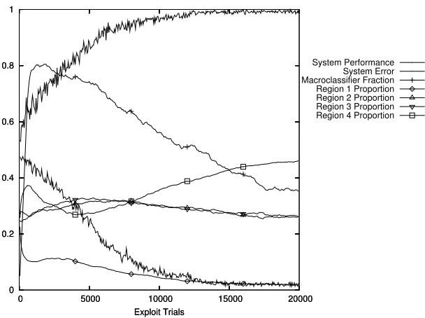
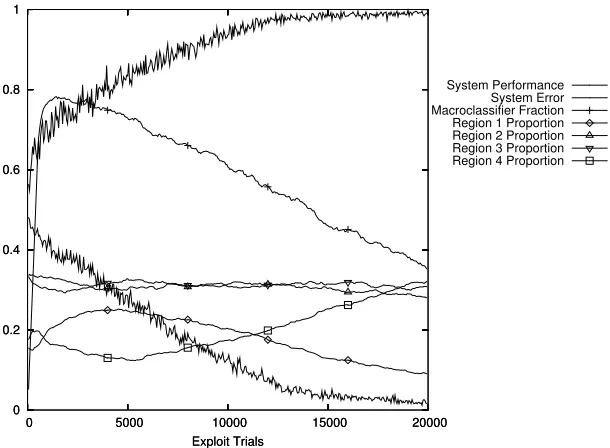
Wilson showed that XCS was able to solve the 6-bit real multiplexer using Centre-Spread Representation. A duplicate of these results is shown in Figure 1. This shows thesystem performance, the fraction of correct actions averaged over the previous 50 exploit trials, thesystem error, the absolute difference of the payoff and the predicted payoff averaged over the previous 50 exploit trials and themacroclassifier fraction, the fraction of the population that are macroclassifiers. Figure 1 also shows other informa-tion that will be referred to later in the paper.

More recently, Bull, Wyatt and Parmee (2002) have shown that XCS can solve the 11-bit real multiplexer.

3 Centre-Spread Representation

To extend XCS into continuous-valued environments, Wilson (2000) introduced the CentSpread Representation. CentSpread Representation provides a form of re-ceptive field for Learning Classifier Systems. An interval predicate,[pi, qi)p, is

repre-sented as a tuple(ci, si)whereci, si ∈ <. ciencodes the centre of the interval andsi

encodes the spread (or width) of the interval. The interval is decoded as follows:

pi = min(pmin, ci−si) qi = max(qmax, ci+si)

Use of Centre-Spread Representation thus involves a genotype(ci, si)to

pheno-type[pi, qi)pmapping, or gene expression.

0 0.2 0.4 0.6 0.8 1

0 5000 10000 15000 20000

Exploit Trials 0

0.2 0.4 0.6 0.8 1

0 5000 10000 15000 20000

Exploit Trials

System Performance System Error Macroclassifier Fraction Region 1 Proportion Region 2 Proportion Region 3 Proportion Region 4 Proportion

Figure 1: 6-bit real multiplexer with Centre-Spread Representation, standard cover withs0= 1, 2-point crossover and standard mutation

we assume a one ofmbinary encoding where the real values for both the centre and spread are encoded into binary integers of lengthkusing the equation

₍₂k

−1)(pi−pmin)

qmax−pmin

With this scheme, the real values for centres and spreads are discretized into one of mpossible values upon encoding. There are22k possible centre-spread combinations and each possible centre-spread is represented exactly once. Because of the discretiza-tion of the phenotype, the half-open soludiscretiza-tion space[pmin, qmax)p in phenotype space

may be regarded as the closed solution space[0,2k

−1]gin genotype space.

The ternary representation used in most Learning Classifier Systems has an ex-plicit ‘don’t care’ value in the form of the ‘#’ allele. Centre-Spread Representation does not have any explicit ‘don’t care’ scheme. Instead, the maximally general inter-val[pmin, qmax)pprovides an implicit ‘don’t care’ mechanism by matching all possible

environmental inputs. An implication of this is that the proportion of maximally gen-eral intervals introduced into the population is not directly controllable by a system parameter, as is normally the case with a ternary representation.

3.2 Properties

As the solution space is half-open, the centre-spread genotype must be limited upon expression in order to restrict the range of the phenotype to the interval[pmin, qmax)p.

We refer to this process astruncation. Truncation means that the genotype to phenotype (g→p) mapping is non-linear and many to one. In short, it is possible for a phenotype to be represented by more than one genotype. As an example, consider the solution space interval[0,1)p. The phenotype[0.5,1)pmay be represented as centre-spread

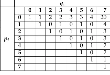
Table 1: Phenotype frequency matrix for Centre-Spread Representation withk= 3

qi

0 1 2 3 4 5 6 7

0 1 1 2 2 3 3 4 20

1 1 0 1 0 1 0 4

2 1 0 1 0 1 3

pi 3 1 0 1 0 3

4 1 0 1 2

5 1 0 2

6 1 1

7 1

In practice, the number of possible centre-spread tuples representing an interval is finite, due to the discretization necessary when representing real numbers. The number of possible genotypes for a particular phenotype is therefore determined by both the phenotype itself and the details of the encoding of real numbers employed.

If there were no truncation on g _→ pmapping (and thus a one to oneg _→ p mapping), there would be22k_{possible phenotypes. However, given the need for}

trun-cation, certain phenotypes are expressed from multiple genotypes. There are therefore less than22k_{unique phenotypes with the Centre-Spread Representation. Certain}

phe-notypes are ‘missing’ and we refer here to these missing phenotype to genotype (p→g) mappings asholes.

The above two properties mean that using Centre-Spread Representation:

1. Expression of random genotypes results in increased frequency of expression of certain phenotypes over other possible phenotypes.

2. The phenotype space contains holes where certain phenotypes are missing, as they are not expressible.

To examine these phenomena in more detail we enumerated theg _→pmapping for one ofmbinary encodings of length2_≤k_≤12. Without loss of generality,pmin= 0 andqmax= 2k−1.

As a readily understandable example of one of these enumerations, Table 1 shows the frequency of each possible phenotype fork= 3, a 3-bit one ofmbinary encoding of real values1_.

The phenotypic frequency in Table 1 shows several interesting properties:

1. The frequency of all possible phenotype intervals is not uniform (as already dis-cussed).

2. Certain phenotype intervals have zero frequency (as already discussed).

3. The frequency of an exact number[pi, pi]pis always 1.

4. The frequency of intervals of the form[pmin, qi)pincreases asqiincreases and the

frequency of intervals of the form[pi, qmax)pincreases aspidecreases.

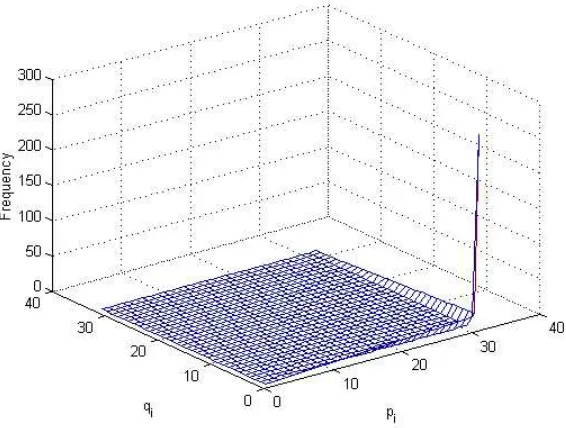
Figure 2: Phenotype frequency landscape for Centre-Spread Representation withk= 5

5. The frequency of the[pmin, qmax)pinterval is much greater than any other.

All encodings2≤k≤12show the same patterns and properties. Only the specific frequencies vary. Space does not permit the publication of the details of each of these, but as a further example and aid to visualization, Figure 2 shows the frequency matrix fork= 5plotted as a surface that may be viewed as the landscape of theg_→pmapping for that particular encoding.

From these results, we can state certain properties of the Centre-Spread Represen-tation.

Property 1: Many to one genotype to phenotype mapping. This property is the key property from which all others derive and has already been discussed in detail.

Property 2: Incomplete phenotype to genotype mapping. A corollary of the discretiza-tion of the centre and spread and the many to oneg_→pmapping (Property 1) is that thep→gmapping is undefined for certain phenotypes.

Holes arise because of the discretization of the encoding:

1. The centre must be located at a point that can be represented using the discrete encoding (i.e., it must be integer-valued).

2. The spread must be able to be represented using the discrete encoding (it must also be integer-valued).

For example, consider interval[1,2]pin Table 1. This interval cannot be represented

In general, any interval whereqi −pi is odd is unable to be represented using

Centre-Spread Representation. Because of this, where holes exist in the g _→ p mapping, they are uniformly distributed around the solution space, such that they are neighbours with ag→pmapping that has non-zero frequency (i.e., is a one-to-one or many-to-one-to-one mapping). No two holes are ever situated next to each other. The presence of holes is undesirable in theg → pmapping, since it means that certain phenotypes cannot be expressed. This, in turn, means that the accuracy of an expressed phenotype is lower than it would otherwise be since the effective discretization of the phenotype is coarser than desired. However, the fact that holes are always located next to a phenotype that can be expressed places a lower limit on the effective discretization of the Centre-Spread Representation.

Holes are an artefact from using one ofmbinary encoding. With a floating point encoding, the holes would be small enough to cause no practical problems.

Property 3: The genotype to phenotype mapping of exact numbers is one to one. In-tervals of the form[pi, pi]p are the leading diagonal of the frequency matrix and

represent exact numbers or points in the solution space. These may be necessary to represent a solution in a particular problem and always have frequency one (i.e., a one-to-oneg→pmapping). A corollary of this is that all possible exact numbers can be represented using Centre-Spread Representation.

Property 4: The frequency of intervals of the form[pmin, qi)p and[pi, qmax)p increases

aspi decreases orqi increases. Property 1 states that certain phenotypes can be

expressed from multiple genotypes. Property 4 provides more detail on the nature of this many to one mapping.

As seen in Figure 2, theg_→plandscape is characterized by a flat plateau contain-ing the majority ofg _→pmappings. These exist with a frequency of either 0 or 1 (i.e., not expressible, or one-to-one mapping). All of the one-to-manyg_→p map-pings occur in phenotypes of the form[pmin, qi)por[pi, qmax)p. The special case of

the[pmin, qmax)pphenotype is discussed in Property 5.

Moreover, the frequency of mappings increases as either pi decreases or qi

in-creases. Thus, wide (general) intervals ‘anchored’ atpmin orqmax have a greater frequency of expression than narrow (specific) intervals or those not anchored at pminorqmax.

Property 5: The frequency of the[pmin, qmax)pinterval is much greater than that of any

other interval. Property 4 states that the expression frequency of intervals of the form[pmin, qi)p and[pi, qmax)p increases aspi decreases orqiincreases. A special

case of this is the interval[pmin, qmax)p. The expression frequency of this interval is

much larger than any other and it completely dominates theg _→plandscape, as shown in Figure 2.

The [pmin, qmax)p interval has special significance for interval-based

representa-tions, as it describes the maximally general interval predicate. A consequence of Property 5 is that randomly generated genotypes will be expressed as the maxi-mally general interval predicate with a far higher frequency that would otherwise be expected.

From examination of the results of enumerating the expression frequencies for real encodings of length 2 _≤ k _≤ 12, we can derive equations for the total frequency of expression of all possible intervals of the form[pmin, qi)pand[pi, qmax)p:

fpmin,qi= 2

2(k−1)

∀pmin≤qi< qmax

fpi,qmax = 2 2(k−1)

∀pmin< pi≤qmax and frequency of expression of the[pmin, qmax)pinterval:

fpmin,qmax= 2

2(k−1)_{+ 2}k−1

The number of possibleg → pmappings is22k, so the probabilitiesPpmin,qi and Ppi,qmaxof expression of intervals of the form[pmin, qi)pand[pi, qmax)prespectively, is

given by

Ppmin,qi =

22(k−1)

22k

= 2 k−1

2k+1

= 0.25

and similarly,Ppi,qmax= 0.25

The probability Ppmin,qmax of expression of the maximally general interval

[pmin, qmax)pis given by

Ppmin,qmax =

22(k−1)_{+ 2}k−1

22k

= 2 k−1_{+ 1}

2k+1

lim k→∞ =

2k−1

2k+1 (1)

= 0.25

Although Equation 1 describes limiting behaviour for infinite length encoding of real numbers, actual values ofPpmin,qmax are close to 0.25 for values ofk likely to be

used in practice (8, 16 or 32 bit encodings). For example, fork= 8,Ppmin,qmax= 0.25195

and fork= 16,Ppmin,qmax= 0.25001.

Ppmin,qmax is the probability of the interval[pmin, qmax)pbeing expressed ong →p

mapping of a random genotype. Centre-Spread Representation thus includes a form of implicit ‘don’t care’ mechanism, similar to that of the ‘#’ allele in ternary representa-tions. However, unlike ternary representations thisP#value is fixed at 0.25 and so is not adjustable to suit different problems.

The probability of expression of an interval of the form

[pi, qi)p∀pi =pmin∨qi=qmax is

Table 2: Phenotype regions and their structural forms

qi

pi Region 2[pmin, qi)p Region 4[pmin, qmax)p

Region 1[pi, qi)p Region 3[pi, qmax)p

This value is essentially independent of encoding length.

So these ‘special’ phenotypes constitute 75% of allg→pmappings, yet only com-prise2k+1−1of the22kpossibleg→pmappings. Their frequency therefore far exceeds what might be reasonably expected for ag _→ pmapping. In contrast, all remaining g _→pmappings of the form[pi, qi)p ∀pi > pmin∧qi< qmax(the plateau in theg→p landscape) constitute only the remaining 25% of all mappings.

We can partition the phenotype space into four regions corresponding to the four different structural forms of interval predicate resulting from the properties of the en-coding. Table 2 shows the four structural forms of interval predicate, together with the region number we shall, for convenience, assign to them. This diagram mimics the shape of the phenotype frequency matrix and shows the allocation ofg _→pmappings by region. In the diagram and the rest of this paper, unless otherwise noted,

pmin< pi≤qmax ∧ pmin≤qi < qmax

3.3 Operators

Since the real multiplexer is essentially a binary problem in disguise, solutions to the real multiplexer are expressed by an alphabet of three possible interval predicates di-rectly corresponding to the Boolean multiplexer’s{0,1,#}alphabet. For the real multi-plexer, the solution interval predicates are{[0, θi)p,[θi,1)p,[0,1)p}. However, these are

exactly the forms of interval predicate found in regions 2, 3 and 4 of Table 2 that exhibit many to oneg _→ pmappings and account for 75% of allg _→ pmappings! We may therefore expect that the choice of Centre-Spread Representation has a bearing on XCS’ ability to solve the real multiplexer problem.

There are four places where the influence of the representation is felt in a Learning Classifier System: initialization, covering, crossover and mutation. We note that, for continuous-valued representations, GA subsumption is performed at the level of the phenotype and is independent of the representation in use.

3.3.1 Initialization

Where a population is generated at random by genotype, a non-uniformg _→ p map-ping will affect the proportion of phenotypes expressed by the population. For Centre-Spread Representation, generation of random genotypes at initialization time will pro-vide a population containing on average a proportion of

1₋ 1

4n (2)

0.9998. In contrast, a one to oneg_→pmapping would provide a proportion of (n−2)2_{+ 1}

n2

Forn= 6this is 0.472. We note here that Figure 1 shows results obtained without an initial population.

3.3.2 Covering

In XCS’ cover operator, the centre of the interval is fixed by the environmental state. For the real multiplexer problem, the environmental state is externally generated from the uniform probability distributionU[0,1). The cover operator for Centre-Spread Rep-resentation generates the spread from the uniform probability distributionU[0, s0). In Wilson’s experiments s0 = 1, so any spread0 ≤ si < 1is equally possible.

There-fore, both centre and spread are drawn fromU[0,1), so all possible centre-spreads are equally probable and the probabilitiesPpmin,qi,Ppi,qmaxandPpmin,qmaxalso apply during

covering. The cover operator, like initialization, thus generates classifiers with a 0.75 probability of being in region 2, 3 or 4 and that have a probability given by Equation 2 of one or more intervals of the correct structural form to solve the problem.

3.3.3 Crossover

We have determined the probability distribution for new classifiers generated by the initialization and cover operators. As it is applied with high probability, crossover has the opportunity to affect this distribution by its production of offspring. We examine the impact of crossover on a single interval predicate, represented as a centre-spread tuple. We are only interested in the action of crossoverwhen it occursfor a specific interval predicate. For crossover to alter that interval, a crossover point must occur within the interval. All the crossover operators considered in this paper that allow a crossover point within an interval restrict the crossover point to occur between the two alleles representing the interval. If the crossover point happens to occur between intervals, the interval itself survives unscathed (although it is likely to be paired with other intervals).

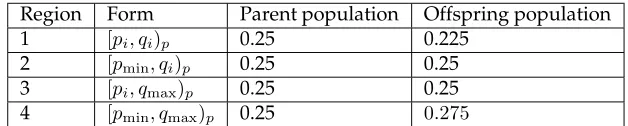
As mathematical analysis of crossover is difficult, we enumerate centre-spread combinations for two parents. We enumerate only those parental intervals that have at least one point in common with each other, since XCS uses a niche GA. A factor in the enumeration is the length of the real encoding used. For consistency with the re-sults presented for mutation, we used an encoding of lengthk = 8and crossed over a single centre and spread with a fixed crossover point between the alleles. For each combination, we noted the region(s) that the parents occupied and the region(s) occu-pied by their children. Enumeration of all possible centre-spread combinations implies an equal probability of parental intervals across the four regions. As already discussed, this is the case for intervals generated by initialization and covering. From this we may readily calculate the expected proportions of offspring across regions. This is shown in Table 3.

Table 3: Phenotype proportions for Centre-Spread Representation with k = 8 and crossover within an interval

Region Form Parent population Offspring population

1 [pi, qi)p 0.25 0.225

2 [pmin, qi)p 0.25 0.25

3 [pi, qmax)p 0.25 0.25

4 [pmin, qmax)p 0.25 0.275

3.3.4 Mutation

The mutation operator for XCS with Centre-Spread Representation mutates a classifier by adding or subtracting with equal probability an amountmidrawn fromU[0, m). A

setting ofm= 0.1was used for Wilson’s real multiplexer experiments.

We examine the behaviour of mutation over the four regions by studying the prob-ability of an offspring occupying a region, given each possible parental region. To do this, we enumerate all possible mutations for an interval using a setting ofm= 0.1for every centre-spread combination over a range of possible values ofk, the real encoding length. In the actual Learning Classifier System, the alleles corresponding to the inter-val’s centre and spread are independently mutated with probabilityµ, so we examine these separately. Mutation of the centre allele shifts the centre by the amount of the mutation, viz:

pi = ci−si+mi qi = ci+si+mi

Mutation of the spread allele alters the width of the interval:

pi = ci−si−mi qi = ci+si+mi

For brevity, and since both centre or spread alleles have equal probability of mu-tation, we average the individual results from these enumerations to provide a picture of the effect of a single mutation on the interval predicate2_{. Mutations for values of}

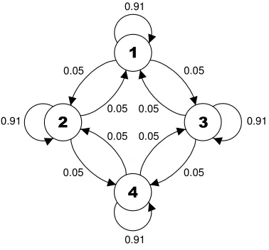
4_≤k_≤8were examined, and a common pattern was seen across all enumerations. As an illustration of the results found, Figure 3 shows the transition diagram of a single mutation of the interval predicate fork = 8. In the diagram, the states are the four possible regions that the parent could occupy and the numbers next to the arrows in-dicate the probability of a transition to a particular region for the offspring. As these probabilities are rounded to two decimal places, we do not distinguish here between very low probabilities (<0.01) and zero probability.

We can see from the diagram that the vast majority of all possible mutations do not produce any migration of region between the parent and offspring (where a re-gion maps to itself). A parent tends to generate offspring that occupy the same rere-gion as itself, so parents with the correct structural form of the real multiplexer solution, [pmin, qi)p, [pi, qmax)p and [pmin, qmax)p, will overwhelmingly produce offspring with

0.91

0.91 0.91

0.91

0.05 0.05

0.05 0.05 0.05 0.05

0.05 0.05

Figure 3: Region transition diagram for Centre-Spread Representation withk= 8and standard mutation. Regions are represented by states and transition probabilities by arrows

It is possible for mutation to produce offspring that occupy a different region to that of the parent, but this occurs with a low probability. Migration between regions is pos-sible via the two pathways1↔ 2↔ 4and1 ↔ 3↔ 4through which offspring are likely to progress through multiple mutation steps. These represent a partial ordering of regions. It is possible to travel in both directions along these pathways with roughly equal probability, showing that this mutation operator is broadly neutral with respect to transitions across regions.

4 Ordered Bound Representation

Wilson (2001a) introduces a representation that describes an interval predicate by its lower and upper endpoints. This is used for problems requiring integer variables. However, when using a one ofmbinary encoding for real variables, the encoding for real numbers differs from that of integers only in the size of the alphabet used and the consequent size of the genotypic search space. There is no reason why the Ordered Bound Representation cannot also be used for continuous-valued problems and, in-deed, the same representation is also used for real-valued function approximation in (Wilson, 2001b).

Ordered Bound Representation stores an interval predicate [pi, qi)p as a tuple (li, ui)where for real-valued problemsli, ui ∈ <. li is the lower bound of the

inter-val anduiis the upper bound. We again assume that the alleles are encoded using a

one ofmbinary encoding of lengthk.

One issue with Ordered Bound Representation is the ordering imposed on the alleles representing an interval predicate by the restriction thatli≤ui. Wilson does not

and swap the lower and upper alleles if the orderingli ≤uiis violated as a result of

the operation.

Apart from discretization in the real encoding, there is a direct mapping between the elements of the genotype and phenotype, so thatli ≡pi andui ≡qi. As a result,

no explicit gene expression is necessary and, at the level of the representation, a one to one mapping exists for all possible phenotypes and their corresponding genotypes. No truncation occurs upon the expression since it is not possible to represent values outside the endpoints of the phenotype interval[pmin, qmax)p. The issues arising from

the many to oneg _→pmapping with Centre-Spread Representation cannot arise with Ordered Bound Representation.

4.2 Properties

In Section 3.2 we stated certain properties that exist due to the many to oneg → p mapping of Centre-Spread Representation. For reference, the equivalent properties of Ordered Bound Representation are:

Property 1: One to one genotype to phenotype mapping.

Property 2: Complete phenotype to genotype mapping.

Property 3: The genotype to phenotype mapping of exact numbers is one to one.

Property 4: The frequency of intervals of the form[pmin, qi)pand[pi, qmax)pis constant

for allpiandqi.

Property 5: The frequency of the[pmin, qmax)pinterval is the same as that of any other

interval.

These are all due to the one to oneg→pmapping that exists for Ordered Bound Representation. The representation stores all possible interval predicates with equal frequency and shows no bias towards certain types of interval predicate. This sug-gests that Ordered Bound Representation may be more suited for continuous-valued domains where the structure of the problem isa prioriunknown.

The maximally general interval [pmin, qmax)p is represented by a single tuple in

Ordered Bound Representation, so given a random genotype, an interval predicate will be maximally general with probability

1 22k

As the sizekof the real number encoding increases and thus its granularity be-comes finer, the chances of a maximally general interval appearing in the initial pop-ulation becomes exponentially lower. This is in contrast to the Centre-Spread Repre-sentation, which results in the maximally general interval being represented with an essentially fixed probability of 0.25. For this reason, Ordered Bound Representation effectively provides no implicit ‘don’t care’ mechanism analogous to the ‘#’ allele in a ternary representation.

4.3 Operators

4.3.1 Initialization

Where a population is generated at random by genotype, a uniformg _→ pmapping across intervals means that all possible phenotypes will exist in the population with identical probability. The frequency of expression of intervals of the form[pmin, qi)p, [pi, qmax)pand[pmin, qmax)p(regions 2, 3, and 4) can be calculated as

fpmin,qi = 2 k

−1_∀pmin≤qi< qmax

fpi,qmax = 2

k

−1_∀pmin< pi≤qmax

fpmin,qmax = 1

The number of possible g → pmappings whereli ≤ ui is2k−1(2k + 1), so the

frequency of intervals of the form[pi, qi)p∀pi> pmin∧qi< qmax(region 1) is given by

fpi,qi = 2

k−1₍₂k_{+ 1)}

−2(2k

−1)₋1 = (2k−1)(2k−1−1)

The probability of expression of an interval of this form is

Ppi,qi = (2k

−1)(2k−1 −1) 2k−1₍₂k_{+ 1)}

= 2

2k−1₋₃₍₂k−1_{) + 1}

22k−1_{+ 2}k−1

lim

k→∞ = 1

Initialization therefore generates classifiers essentially exclusively in region 1. No classifiers are to be expected in a small, finite, population with the correct structural form of the solution as occurs in Centre-Spread Representation.

4.3.2 Covering

The cover operator generates a classifier containing intervals with the (li, ui)tuples

given by

li = xi−U[0, s0)

ui = xi+U[0, s0)

To match the experiments performed with Centre-Spread Representation3_s

0= 1. Note that, unlike the case with Centre-Spread Representation, the resulting interval is not generally centred on the environmental variable,xi. This is the method adopted

by Wilson, which we also use here. However, it would be trivial to alter the algorithm to emulate Centre-Spread Representation strategy by using the same random spread for both endpoints and this is examined in Section 9.2. In either case, truncation is necessary when mapping from the generated interval to the genotype. This truncation causes similar effects to those seen for Centre-Spread Representation. For example, Table 4 shows the frequency matrix for all possible intervals generated by the cover operator using a real encoding of length ofk= 3.

This shows increased frequency of regions 2, 3 and 4 similar to that of Centre-Spread Representation. Furthermore, region 1 also shows increased mapping fre-quency as the interval widthqi−pi increases. Studies of such matrices for encoding

3_{(Wilson, 2001a) refers to the cover spread asr}

Table 4: Phenotype frequency matrix for Ordered Bound Representation with k = 3 and standard cover withs0= 1

qi

0 1 2 3 4 5 6 7

0 8 15 21 26 30 33 35 120

1 1 2 3 4 5 6 35

2 1 2 3 4 5 33

pi 3 1 2 3 4 30

4 1 2 3 26

5 1 2 21

6 1 15

7 8

lengths of2 _≤ k _≤ 8all showed the same effects. From these we can derive the fre-quencies of expression of the region 2, 3 and 4 intervals:

fpmin,qi = 23k

−2k 3

fpi,qmax =

23k

−2k 3

fpmin,qmax =

(2k_{+ 1)}3 −2k

−1 6

and the probabilitiesPpmin,qi, Ppi,qmax and Ppmin,qmax for the cover operator with

Or-dered Bound Representation:

Ppmin,qi =

23k₋₂k 3(23k₎

= 1 3−

1 3(22k₎

lim n→∞ =

1 3

and similarly,Ppi,qmax= 1 3

Ppmin,qmax =

(2k+ 1)3−2k−1 6(23k₎

lim n→∞ =

1 6 thusPpi,qi =

1 6

So, even though Ordered Bound Representation has no intrinsic bias, the trunca-tion necessary when using the cover operator introduces bias. This is shown in Figure 4 fork= 5.

Figure 4: Phenotype frequency landscape for Ordered Bound Representation with k= 5and standard cover withs0= 1

Table 5: Phenotype proportions for Ordered Bound Representation withk = 8and crossover within an interval

Region Form Parent population Offspring population

1 [pi, qi)p 0.25 0.984

2 [pmin, qi)p 0.25 0.008

3 [pi, qmax)p 0.25 0.008

4 [pmin, qmax)p 0.25 <0.001

setting ofs0= 1provides a good bias for the real multiplexer problem since it generates classifiers with one or more intervals of the correct structural form (i.e., those in regions 2, 3 and 4) with a probability of

1₋ 1 6n

For the 6-bit real multiplexer, this probability is 0.99998.

4.3.3 Crossover

Analysis of crossover with Ordered Bound Representation for an encoding of length k= 8as described in Section 3.3.3 yields the results shown in Table 5.

Repre-1.00

0.96 0.95

0.93

0 0

0.04 0.04 0.04 0.05

0 0

Figure 5: Region transition diagram for Ordered Bound Representation withk= 8and standard mutation. Regions are represented by states and transition probabilities by arrows

sentation (Section 4.3.1). For simplicity, the analysis assumes a parent population with a uniform distribution across regions, which is not generally the case. But, although exact details will vary, the general trends seen here should still apply.

4.3.4 Mutation

Mutation for Ordered Bound Representation was studied in the same way as for Centre-Spread Representation (Section 3.3.4). The transition diagram for k = 8 is shown in Figure 5.

This displays similar characteristics to those of Centre-Spread Representation. Most mutations cause no change of region from parent to offspring, but simply refine the details of the interval within the region. When a transition does occur, the transi-tion probabilities for Ordered Bound Representatransi-tion essentially only allow transitransi-tions away from anchored (region 2, 3 and 4) intervals.

5 Unordered Bound Representation

Ordered Bound Representation provides a one to oneg _→pmapping, but theli ≤ui

ordering restriction is unnecessary. If this restriction is lifted, the phenotype can still be directly encoded using the endpoints of the interval, but without an ordering require-ment. Thus, an interval[pi, qi)pmay be encoded as the tuples(pi, qi)or(qi, pi)∀pi6=qi.

0 0.2 0.4 0.6 0.8 1

0 5000 10000 15000 20000

Exploit Trials 0

0.2 0.4 0.6 0.8 1

0 5000 10000 15000 20000

Exploit Trials

System Performance System Error Macroclassifier Fraction Region 1 Proportion Region 2 Proportion Region 3 Proportion Region 4 Proportion

Figure 6: 6-bit real multiplexer with Unordered Bound Representation, standard cover withs0= 1, 2-point crossover and standard mutation

suggests that the solution to a problem using an interval-based representation is best expressed in the form of a vector of intervals, rather than simple inequalities, so any resulting slight performance differences compared to Ordered Bound Representation should, if anything, be advantageous. In any event, the bias induced by the Unordered Bound Representation’sg→pmapping is negligible compared to the major disparities in phenotype expression frequency seen using Centre-Spread Representation.

The advantage of Unordered Bound Representation over Ordered Bound Repre-sentation is that it avoids the additional operator complexity associated with swapping the endpoints of an interval if theli≤uiordering restriction is violated. Although this

may seem trivial, the presence of the ordering restriction constitutes a form of epista-sis between theli anduialleles, as their values are mutually dependent. A resulting

swap may generate great change in a particular locus when viewed before and after the operation that caused the swap to occur. This cannot occur using Unordered Bound Representation, since no ordering of endpoints exists for the interval predicate at the level of the genotype.

Figure 6 shows the results of using Unordered Bound Representation on the 6-bit real multiplexer problem.

5.2 Properties

Properties of Unordered Bound Representation are:

Property 1: Two to one genotype to phenotype mapping for intervals (but not exact numbers)

Property 2: Complete phenotype to genotype mapping.

Property 4: The frequency of intervals of the form[pmin, qi)pand[pi, qmax)pis constant

for allpiandqi.

Property 5: The frequency of the[pmin, qmax)pinterval is the same as that of any other

interval.

The maximally general interval[pmin, qmax)pmay be represented by two possible tuples

in Unordered Bound Representation, so given a random genotype, an interval will be maximally general with probability

1 22k−1

Thus, Unordered Bound Representation, like Ordered Bound Representation, pro-vides no implicit ‘don’t care’ mechanism.

5.3 Operators

In this section we investigate Unordered Bound Representation and the operators adapted for it.

5.3.1 Initialization

The frequency of expression of intervals of the form [pmin, qi)p, [pi, qmax)p and [pmin, qmax)p(regions 2, 3, and 4) can be calculated as

fpmin,qi = 2 k+1

−3_∀pmin≤qi< qmax

fpi,qmax = 2

k+1

−3_∀pmin< pi ≤qmax

fpmin,qmax = 2

The number of possibleg_→pmappings is22k_{, so the frequency of intervals of the}

form[pi, qi)p∀pi> pmin∧qi< qmax(region 1) is given by

fpi,qi = 2

2k

−2(2k+1₋3)₋2 = (2k

−2)2

The probability of expression of an interval of this form is

Ppi,qi = (2k

−2)2

22k

= 2

2k

−2(2k+1_{) + 4}

22k lim

n→∞ = 1

The implication of this is that, like Ordered Bound Representation, initialization generates classifiers essentially exclusively in region 1.

5.3.2 Covering

0.95

0.74 0.74

0.51

0.02 0.02

0.25 0.25 0.25 0.25

0.01 0.01

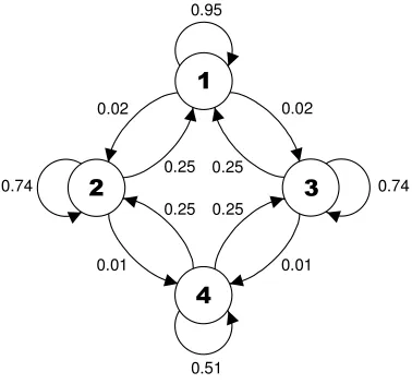
Figure 7: Region transition diagram for Unordered Bound Representation withk = 8 and standard mutation. Regions are represented by states and transition probabilities by arrows

5.3.3 Crossover

Analysis of crossover with Unordered Bound Representation for an encoding of length k = 8as described in Section 3.3.3 yields the same results as those shown in Table 5. The comments made in Section 4.3.3 for crossover with Ordered Bound Representation therefore also apply to Unordered Bound Representation.

5.3.4 Mutation

Mutation for Unordered Bound Representation was studied in the same way as for Centre-Spread Representation (Section 3.3.4). The region transition diagram fork= 8 is shown in Figure 7.

This shows that the mutation operator for Unordered Bound Representation acts to provide a strong pressure away from region 4. For region 4 intervals, there is only a 0.51 probability of staying in region 4 upon mutation, with a transition to regions 2 or 3 equally likely. Similarly for a region 2 or 3 interval, a transition to region 1 is possible with a probability of 0.25.

6 The Real Multiplexer Revisited

of the correct structural form,[pmin, qi)p,[pi, qmax)p and[pmin, qmax)p(regions 2, 3, and

4). Crossover and mutation then refine these by discovering the correct thresholds,θi

to solve the problem. Having one of the endpoints of an interval correct upon initial generation of a classifier allows a much simpler genetic search compared to having to discover both ends of an interval concurrently. In this way, the representation and/or operators relieve the other mechanisms of XCS from much of the burden of solving the real multiplexer problem because the solution to the problem happens to match the nature of the classifiers being generated. But, for an arbitrary problem, this may not be the case.

6.2 Sampling Bias

This hypothesis suggests that the time taken to solve the real multiplexer problem should be independent of the threshold,θi. We repeated the real multiplexer

experi-ment in (Wilson, 2000) whereθi= 0.75and, like Wilson, were unable to solve the

prob-lem in 20,000 exploit trials. However, we found that if XCS is allowed to run for 50,000 trials, it does solve the problem. In fact, XCS takes approximately 2.5 times longer to solve the real multiplexer withθi = 0.75, than whenθi = 0.5, even ifθi = 0.75does

not alternate across values ofi. Further experimentation revealed that this is because [0,0.75]p intervals are sampled with three times the frequency than that of [0.75,1)p

intervals. If both intervals are sampled with equal frequency, then XCS solves the problem in the same number of trials as for whenθi = 0.5(not shown). This is the

explanation that Wilson suggests. Importantly, the difference in performance solely arises due to sampling bias and not from any representation or operator bias present.

6.3 Relationship to Integer Results

Even with a neutral representation, such as Ordered Bound Representation or Un-ordered Bound Representation, the present cover operator still generates classifiers containing intervals with the correct structural form with an increased frequency. The Random-Data2 and Random-Data9 test problems (Wilson, 2001a) exhibit the same characteristics as described for the real multiplexer; that is, solutions to the problem are of the form [pmin, qi)p,[pi, qmax)p and[pmin, qmax)p(regions 2, 3, and 4). It would

appear from Wisconsin Breast Cancer results4_{that this problem also has these}

charac-teristics. Wilson asks why XCS solves the Random-Data9 problem within a factor of 10 of the simpler Random-Data2 problem when the input space is exponentially larger (109_versus102_{). We hypothesize that the covering bias described plays a part in this} anomaly by generating classifiers containing intervals of the correct structural form. It is not unreasonable then to assume that the additional effort for crossover and muta-tion to refine these is better than exponential. Further work is necessary to validate this hypothesis with the above test problems.

6.4 Interval Predicates and the Real Multiplexer

We suggest that the real multiplexer problem is a poor choice of test problem for Learn-ing Classifier Systems operatLearn-ing with continuous-valued data and interval predicates, since its solutions all have one endpoint in common with the maximally general inter-val in the solution space. Because of this, it is not representative of the broader class of problem where solutions are not, in general, closely aligned to the representation of the ‘don’t care’ state.

Figure 8: Rectangle centred in a 2-dimensional solution space. The decision surface is shaded

The benefits of interval predicates are that they are able to represent hyper-rectangular decision surfaces in solution space. These benefits only accrue if (i) the problem solution requires a hyper-rectangle, rather than a hyperplane decision surface or (ii) the form of the problem solution is not knowna priori. The real multiplexer prob-lem can be solved using a hyperplane decision surface since all of the hyper-rectangles needed for the solution are anchored at a boundary of the solution space. It does not strictly require the presence of interval predicates to represent the solution and conse-quently cannot adequately test the general operation and performance of representa-tions that use interval predicates.

We argue that the real benefit of the use of interval predicates is their ability to represent arbitrary intervals in solution space. This provides a richer expressive power that cannot be achieved using hyperplane Decision Surfaces and potentially allows a broader class of problem to be solved. In many real-world problems, the form of the solution is unknowna priori and test problems for Learning Classifier Systems using interval predicates must be flexible enough to explore all aspects of their operation and performance. This is not the case with the real multiplexer problem.

7 Hyper-Rectangles

7.1 Full Environmental Map

XCS attempts to build a full environmental map of the problem in order to cover the solution space with classifiers. The map takes the form of the population of classifiers, with individual classifiers representing portions of the map.

Classifiers using an interval-based representation construct hyper-rectangular de-cision surfaces in solution space. For all of the problems discussed in Section 6, the decision surface can be represented by a hyperplane and so one of the faces of the hyper-rectangle is always at the boundary of the solution space. This face simply serves to specify the direction of the inequality otherwise represented by the hyperplane.

A rectangle can approximate more complex decision surfaces than a hyper-plane. In this case the decision surface is closed and will have faces that are not at solution space boundaries. This would seem to be a disadvantage for representation and operator combinations that provide bias towards the solution space boundaries. However, since XCS builds a complete map of the solution space, for each classifier representing a closed decision surface, there are multiple classifiers representing the solution space outside the closed decision surface. For example, consider a rectangle centred in a 2-dimensional solution space (Figure 8).

Figure 9: The four types of decision surface representing the solution interval (shaded) possible in a 1-dimensional solution space

7.2 1-Dimensional Solution Space

A single closed decision surface can be created in a 1-dimensional solution space by dividing the solution space into non-overlapping hyper-rectangles in four ways (Fig-ure 9).

In case 1 three hyper-rectangles (i.e., interval predicates) must be constructed to cover the solution space. Two of these have their faces at the solution space boundary (the unshaded rectangles in the diagram). This is the general problemθl ≤ xi < θu,

whereθlandθuare the lower and upper bounds of the solution interval.

For cases 2 & 3 the solution space is covered by two hyper-rectangles, both of which have one of their faces at the solution space boundary. These are the cases for the real multiplexer and the other experiments discussed in Section 6.

Case 4 shows a hyper-rectangle covering all of one dimension of the solution space, with both faces at the boundary of the solution space. This represents the maximally general ‘don’t care’ interval.

Notice that the four cases shown correspond to the four structural forms (regions) of interval predicate previously described.

Thus, for a single closed decision surface representing the solution interval, there are always more hyper-rectangles requiring faces at the solution space boundary than those that do not. This is because XCS ‘fills in’ the missing parts of the solution space when building its complete environmental map. Strictly, this closed decision surface is all that is required for a classifier in a traditional (non-accuracy based) classifier system. However, XCS also generates the other hyper-rectangles to complete the map.

Even if a dimension of the solution space is divided into multiple Decision Sur-faces representing the solution interval, then excluding the maximally general interval (case 4 above), there will always be exactly two hyper-rectangles with faces at the solu-tion space boundary. The number of hyper-rectangles without faces at solusolu-tion space boundaries exceeds those with faces at solution space boundaries only when a dimen-sion of the solution space is divided into a total of five or more hyper-rectangles. Thus, it would seem reasonable to assume that a bias towards hyper-rectangles with faces at solution space boundaries is an advantage when a 1-dimensional solution space is divided into less than five hyper-rectangles.

7.3 Multidimensional Solution Space

Of course, in a multidimensional solution space, the influence of the hyper-rectangle complexity of all dimensions must be taken into account. Assuming that each dimen-sion,n, of the solution space is divided into the same number of hypercubes,nd, the

1 2

3 4

5

0 5

10 0.4 0.5 0.6 0.7 0.8 0.9 1

Divisions Dimensions

P

ro

po

rti

on

Figure 10: Proportion of hypercubes with one or more faces at the solution space boundary for problems of dimensionn, with each dimension divided intond

hyper-cubes

given by

nn

d −(nd−2)n nn

d

∀nd≥2

This is plotted in Figure 10, which shows that the proportion of hypercubes with one or more faces at the solution space boundary depends primarily on the dimension-ality of the problem and only secondarily on the number of hypercubes into which each dimension is divided. For almost all problems, this proportion is greater than 0.5, while for problems with several dimensions (i.e., most real-world problems) the number of hypercubes with no face at the solution space boundary becomes insignificantly small. As a result, these hypercubes are likely to have little influence on the performance of XCS when constructing its environmental map. Therefore, even problems where the solution is of the form[pi, qi)p∀pi> pmin∧qi< qmax(region 1) should benefit from the representation and operator bias studied here, as the solution to the problem is domi-nated by the search for intervals in regions 2, 3 and 4 – precisely those for which bias exists.

8 The Checkerboard Problem

diffi-Figure 11: 2-dimensional checkerboard withnd= 5

culty is controlled by both the dimensionality of the solution space,nand the number of divisions of each dimension of the solution space,nd. To allow the colours to

alter-nate in all dimensions,nd must be an odd number. Figure 11 shows a 2-dimensional

checkerboard withnd= 5.

On each trial, the Learning Classifier System is presented with a vector ofn ran-dom real numbers in the interval [0,1)p, representing a point in the solution space.

The Learning Classifier System then attempts to assign an action, 0 or 1 depending on whether the point is contained in a black (0) or white (1) hypercube. The classifiers generated by the Learning Classifier System thus correspond directly to hypercubes in the solution space.

The solution to the checkerboard problem, as presented, requires no maximally general intervals due to the presence of alternating hypercubes. Although we do not use it here, a controlled number of maximally general intervals may be added to the checkerboard problem by making black entire hyper-rows and hyper-columns of the checkerboard. The number of hyper-rows and hyper-columns generalized in this way is controlled by a parameter,ng with the maximally general intervals being allocated

uniform randomly among dimensions and divisions of the problem.

The checkerboard problem is analogous to the test suite for ternary representations detailed in (Kovacs & Kerber, 2001).

8.2 Checkerboard with Initial Population

Figure 12 and Figure 13 show the performance of Centre-Spread Representation and Unordered Bound Representation on the checkerboard problem withn= 3andnd= 3.

The solution to this problem consists of 27 hypercubes, so XCS needs 54 classifiers to construct a full map. In these experiments, an initial population of 2000 classifiers was used. Other settings are as for the real multiplexer experiments. We did not test the performance of Ordered Bound Representation due to its similarity to Unordered Bound Representation.

Here, the initial proportions of intervals in each region of the population match well the theoretically predicted values for initialization. In these experiments, pro-portions of intervals in each region are measured with reference to the macroclassifier population.

By observing the proportions of intervals in the population occupying the four re-gions, it is possible to gain some insight into the dynamics occurring as XCS solves the problem. Notice in Figure 12 (Centre-Spread Representation) how the proportion of each region diverges from the initial value of 0.25. Compare this to Figure 13 (Un-ordered Bound Representation), where the proportions converge from values of 0 (re-gions 2 and 3) and 1 (region 1).

The expected proportions of each region may be calculated for the checkerboard problem with n = 3 andnd = 3by counting the number of hypercubes at the

0 0.2 0.4 0.6 0.8 1

0 20000 40000 60000 80000 100000

Exploit Trials 0

0.2 0.4 0.6 0.8 1

0 20000 40000 60000 80000 100000

Exploit Trials

System Performance System Error Macroclassifier Fraction Region 1 Proportion Region 2 Proportion Region 3 Proportion Region 4 Proportion

Figure 12: Checkerboard problem with Centre-Spread Representation, an initial popu-lation, standard cover withs0= 1, 2-point crossover ‘within’ and standard mutation

is represented by a specific combination of interval regions (for example, a hypercube at a corner of the solution space is represented by three region 2 or 3 intervals, while a hypercube at an edge is represented by two region 2 or 3 intervals and one region 1 interval). From this, we find that the expected proportion of each of region 1, 2 and 3 classifiers is 1

3. It is clear from Figure 13 that although a solution to the problem ap-pears to have been found, the proportion of region 1 classifiers is too high, whereas the proportion of region 2 and 3 classifiers is too low. This is because, apart from a low probability of mutation, the only pressure towards generalization is that provided by the environment via cover spread. With an environment that presents uniform random values, as classifiers become more general (i.e., have wider intervals), the probability of encountering an environmental input that is outside of an existing interval’s range becomes lower and asymptotically approaches zero. Generalization pressure is thus variable and diminishes as XCS gets closer to solving the problem.

Although the dynamics of execution may differ, there is no great difference in Sys-tem Performance and SysSys-tem Error between representations. We found that the pres-ence of an initial population tended to mask the differpres-ences between representations. For this reason, we now focus on comparing representations using experiments with-out an initial population.

8.3 Checkerboard with no Initial Population

Figure 14 and Figure 15 show the same experiments with no initial population. Again, these results show initial proportions of intervals in each region close to the predicted values for the cover operator, given the small sample size due to the empty initial pop-ulation.

0 0.2 0.4 0.6 0.8 1

0 20000 40000 60000 80000 100000

Exploit Trials 0

0.2 0.4 0.6 0.8 1

0 20000 40000 60000 80000 100000

Exploit Trials

System Performance System Error Macroclassifier Fraction Region 1 Proportion Region 2 Proportion Region 3 Proportion Region 4 Proportion

Figure 13: Checkerboard problem with Unordered Bound Representation, an initial population, standard cover withs0= 1, 2-point crossover ‘within’ and standard muta-tion

inroads towards solving the problem, whereas XCS with Unordered Bound Represen-tation comes much closer. This is due to the abnormally high number of region 4 inter-vals and low number of region 1 interinter-vals in the population with Centre-Spread Repre-sentation. For Centre-Spread Representation, covering is used only during the first 50 trials, during which time the number of region 4 (maximally general) intervals rises in the population. For the remaining trials the region 4 intervals in the population cover all environmental inputs and covering is unnecessary. These intervals take over the population and stall the search. In contrast, the search using Unordered Bound Repre-sentation makes progress from the start, correctly promoting region 1 intervals at the expense of those in region 4. In addition, the proportion of region 2 and 3 intervals after 100,000 exploit trials (0.27) is similar to the expected proportion of 0.33, suggesting that many of the cubes at the boundaries of the solution space have been identified. As sug-gested in Section 7.3, it appears that the bias of the Unordered Bound Representation operators and parameter settings better match the type of intervals needed to solve the problem than those of Centre-Spread Representation. In fact, covering generates region 2 and 3 intervals with a probability of1

3, which is exactly the right proportion required by the solution to the problem.

9 Comparing Representations and Operators

0 0.2 0.4 0.6 0.8 1

0 20000 40000 60000 80000 100000

Exploit Trials 0

0.2 0.4 0.6 0.8 1

0 20000 40000 60000 80000 100000

Exploit Trials

System Performance System Error Macroclassifier Fraction Region 1 Proportion Region 2 Proportion Region 3 Proportion Region 4 Proportion

Figure 14: Checkerboard problem with Centre-Spread Representation, standard cover withs0= 1, 2-point crossover ‘within’ and standard mutation

identically for both representations.

Without an initial population, the operators responsible for any performance dif-ferences are covering, crossover and mutation. GA subsumption is performed at the level of the phenotype, so no performance differences can arise from this operator.

For Unordered Bound Representation, truncation during covering and mutation occurs on the alleles representing the lower and upper bound of the interval. This means that an interval in Unordered Bound Representation is limited to[pmin, qmax)p.

When Centre-Spread Representation is used, it is the centre and spread alleles that are truncated during covering and mutation. Therefore, for Centre-Spread Representation, intervals in the underlying population are in the range[2pmin−qmax,2qmax−pmin)p

and further truncation must be applied upon expression to limit these intervals to [pmin, qmax)p. The cover, crossover and mutation operators all work at a genotypic level,

so in the case of Centre-Spread Representation, it is possible for intervals to be main-tained in the population that are outside the range of the phenotype, but which are available for crossover and mutation to manipulate, and from which ‘useful’ intervals within range may subsequently emerge. This feature is not available with Unordered Bound Representation, where all intervals in the population are restricted to the range of the phenotype.

To design operators with identical characteristics for both representations, we need to limit the range of intervals in the population to that of the solution space. We thus refer to these as restricted operators. To test the restricted operators and verify that XCS behaves identically when using them, we ran experiments using restricted cover, no crossover and restricted mutation with both representations on the 6-bit real multi-plexer andn = 3,nd = 3checkerboard problem. These showed the same results and

0 0.2 0.4 0.6 0.8 1

0 20000 40000 60000 80000 100000

Exploit Trials 0

0.2 0.4 0.6 0.8 1

0 20000 40000 60000 80000 100000

Exploit Trials

System Performance System Error Macroclassifier Fraction Region 1 Proportion Region 2 Proportion Region 3 Proportion Region 4 Proportion

Figure 15: Checkerboard problem with Unordered Bound Representation, standard cover withs0= 1, 2-point crossover ‘within’ and standard mutation

To compare the effects of different operator choices, we performed extensive ex-perimentation using the Centre-Spread Representation and Unordered Bound Repre-sentation operators and variants. These are listed in Table 6 and described in more detail in the following sections. Space precludes detailed examination of every com-bination of representation, operator and problem, so we focus instead only on general trends and results of particular interest.

9.2 Cover

We compared three variants of cover operator. Standard cover is the cover operator already described. This differs between Centre-Spread Representation and Unordered Bound Representation in two ways:

1. The Centre-Spread Representation cover operator is symmetric, since by defini-tion, the spread must be equal on both sides of the centre. The Unordered Bound Representation cover operator, as presented, is asymmetric.

2. The Centre-Spread Representation cover operator generates intervals in the range [2pmin−qmax,2qmax−pmin)p while the Unordered Bound Representation cover

operator generates intervals in the range[pmin, qmax)p.

Restricted coveris symmetric and generates intervals in the range[pmin, qmax)p for

both representations. The properties of restricted cover are the same as those described in Section 3.3.2. In the case of Unordered Bound Representation, the only change to the covering algorithm is to apply the same random spread to both sides of the envi-ronmental variable being covered. The algorithm for the Centre-Spread Representation restricted cover operator is more complex:

Table 6: Operators used during comparison of representations and operator variants

Operator Variant Characteristics

Cover StandardRestricted Symmetric (CSR), Asymmetric (UBR)Symmetric

Unbiased Symmetric

Crossover

Standard 1-point Between predicates Standard 2-point Between predicates Standard Uniform Between predicates Restricted 1-point Within predicates Restricted 2-point Within predicates Restricted Uniform Within predicates Mutation Standard_Restricted

l=EncodeandT runcate(xi−si) u=EncodeandT runcate(xi+si) s= (u−l)

2 + (u−l) mod 2 c=l+s

The algorithm generates an interval as a lower and upper bound so that truncation occurs as for Unordered Bound Representation. It then converts the encoded interval back to an encoded centre and spread as needed for Centre-Spread Representation. The spread is incremented by one if it is an odd number to ensure that region 4 intervals are generated in the correct proportion. This is necessary because using a one ofm binary encoding, the range of the maximally general interval[pmin, qmax)p is always

odd. It cannot be represented in Centre-Spread Representation without truncation, as only even ranges can be represented.

Unbiased coveris simply a variant of standard cover with a symmetric spread that is limited toU[0,min(xi−pmin, qmax−xi))p. This avoids the need for truncation, as the

spread is limited to the bounds of the solution space.

We found performance differences between standard Unordered Bound Represen-tation (asymmetric) cover and restricted (symmetric) cover with certain combinations of problem, operators and parameter settings. It is possible that such variation in per-formance arises simply because of the differing nature of the bias of the two types of cover, as seen in Section 3.3.2, Section 5.3.2 and below. Alternatively, it could be related to a bias caused by the fact that asymmetric cover chooses a different random spread for each side of the environmental state, whereas symmetric cover produces an inter-val that is (excepting truncation) centred on the environmental input. Further work is necessary to understand these performance differences in more detail.

Table 7: Phenotype frequency matrix for symmetric cover (Centre-Spread Representa-tion and Unordered Bound RepresentaRepresenta-tion) withk= 3ands0= 0.5

qi

0 1 2 3 4 5 6 7

0 1 1 2 2 2 1 1 0

1 1 0 1 0 1 0 1

2 1 0 1 0 1 1

pi 3 1 0 1 0 2

4 1 0 1 2

5 1 0 2

6 1 1

7 1

Table 8: Phenotype frequency matrix for asymmetric cover (Unordered Bound Repre-sentation) withk= 3ands0= 0.5

qi

0 1 2 3 4 5 6 7

0 4 7 9 10 6 3 1 0

1 1 2 3 4 3 2 1

2 1 2 3 4 3 3

pi 3 1 2 3 4 6

4 1 2 3 10

5 1 2 9

6 1 7

7 4

to oneg →pmappings in region 2 and 3 occur around the median values ofpiandqi

with the frequencies ramping up to these values from the solution bounds. This means that covering is more likely to generate region 2 and 3 intervals with ranges around the median than those with very large or small ranges. In addition, the asymmetric cover operator shows a similar effect for region 1 intervals, which does not occur with the symmetric cover operator.

For both representations, the smaller cover spread was an advantage for the checkerboard problem, but produced poorer performance on the real multiplexer prob-lem. This difference arises because of the need for maximally general intervals in the real multiplexer problem that is not present in the checkerboard problem. If the cover operator is able to generate intervals in region 4, this aids XCS in solving the real mul-tiplexer problem. In contrast it is a handicap for the checkerboard problem, where no region 4 intervals are necessary to solve the problem.

0 0.2 0.4 0.6 0.8 1

0 20000 40000 60000 80000 100000

Exploit Trials 0

0.2 0.4 0.6 0.8 1

0 20000 40000 60000 80000 100000

Exploit Trials

System Performance System Error Macroclassifier Fraction Region 1 Proportion Region 2 Proportion Region 3 Proportion Region 4 Proportion

Figure 16: Checkerboard problem with Centre-Spread Representation, standard cover withs0= 0.5, 2-point crossover ‘within’ and standard mutation

vals of each region in the population. Although the performance differences between different values of cover spread are not always so great, the value of the cover spread does have a significant effect on system dynamics and, ultimately, on performance. For reference and comparison with Figure 15, Figure 17 shows the results for Unordered Bound Representation withs0= 0.5.

Unbiased cover showed similar effects with both representations. Whilst its perfor-mance on the checkerboard problem (Figure 18) was better than covering withs0= 1, it proved totally unsuitable for the real multiplexer problem (Figure 19). In Figure 18 it is possible to see how the proportion of region 1 intervals starts at 100% and then decreases as region 2 and 3 intervals are discovered. This happens only very slowly for the real multiplexer. Here, the proportion of region 2, 3 and 4 intervals needed to solve the problem is very low, even after 20,000 runs, when the problem would have been solved with a biased cover operator (Figure 1).

9.3 Crossover