Model-based prognosis for intergranular corrosion
LISHCHUK, S. V. <http://orcid.org/0000-0002-9989-765X>, AKID, R. and WORDEN, K.
Available from Sheffield Hallam University Research Archive (SHURA) at:
http://shura.shu.ac.uk/1469/
This document is the author deposited version. You are advised to consult the publisher's version if you wish to cite from it.
Published version
LISHCHUK, S. V., AKID, R. and WORDEN, K. (2008). Model-based prognosis for intergranular corrosion. Proc. 4th European Workshop on Structural Health
Monitoring, Krakow, Poland, 340-348.
Copyright and re-use policy
See http://shura.shu.ac.uk/information.html
Model-based prognosis for intergranular corrosion
S.V. Lishchuk1, R. Akid1, K. Worden2
1 Centre for Corrosion Technology, Structural Materials and Integrity Research Centre, Sheffield Hallam University, Norfolk Building, Sheffield S1 1WB, UK.
2 Motion and Control Group, Department of Mechanical Engineering, University of Sheffield, Mappin Street, Sheffield S1 3JD, UK.
Abstract
Among the advantages of Aluminium-based alloys for structural use is their corrosion resistance. However, while Aluminium alloys are highly resistant to uniform (general) corrosion, they are much more susceptible to types of localised corrosion, especially intergranular corrosion, which is a localised attack along the grain boundaries which leaves the grains themselves largely unaffected. In order to estimate the progress of such corrosion in a given sample, it is considered possible to generate a numerical model of some sort. While there has been much effort spent in the development of electrochemistry-based models, the use of grey and black-box models remains largely unexplored. One exception to this is the use of Cellular Automata (CA) models which have recently been exploited to model the progression of uniform corrosion. The object of the current paper is to apply the CA methodology to the case of intergranular corrosion. The first phase of the work has been concerned with generating appropriate CA rules which can qualitatively reproduce observed physics, and this work is reported here. A model is proposed which shows qualitative agreement with experimental data on the advance of the corrosion front.
1. INTRODUCTION
for copper-containing aluminium alloys with high content of copper because of the presence of the depleted zones of copper near the grain boundaries.
To describe the intergranular corrosion theoretically is a complicated problem. The macroscopic modelling of electrochemical reactions in the mean-field approximation fails because at the mesoscopic scale the corrosion process is stochastic, which is manifested, for example, in roughness of the corroded surface, or in random initiation of pitting corrosion.
In order to numerically simulate local corrosion attack on aluminium alloys it is necessary to consider the complex microstructure of the alloy, which includes a high number of structural inhomogeneities. It is necessary to simulate a complex system of inhomogeneous processes and reactions that occur in different scales, especially those electrochemical reactions that trigger the onset of localized corrosion and control the corrosion propagation rate.
A promising approach is to model the progression of intergranular corrosion using cellular automata models. Cellular automata (CA), originally proposed by John von Neumann (see [2]), are a discrete dynamical system, but exhibit many properties of a continuous dynamical system, while being simpler to implement. This property makes them a powerful tool for modelling physical, chemical, and biological systems. In particular, CA have recently been exploited to model the progression of uniform corrosion [3–17].
Córdoba-Torres and colleagues developed a very detailed CA model of a corrosion process that mimics several cathodic and anodic events and allows the effect of different reaction kinetic parameters to be investigated [7]. Their results include forecasting the roughness of the corroding interface from the kinetic parameters [8], simulation of the reactions which are described by fractional-order kinetics rather than mean field approximation [9], and study of the process of spatial segregation of surface reactants in the corrosion process [10].
On the other hand, Vautrin-Ul et al [12] have demonstrated that several features of a corrosion process can be recovered by using a CA model which uses only one parameter. This rather simple model has allowed the complicated behaviour of the system to be simulated and quantitative prediction of the roughness of the system.
To study corrosion pit growth, Malki et al [15] considered the metal-film-electrolyte system as a probabilistic cellular automaton with specific transition rules, which showed that the dissolution probability strongly influences both pit morphology and pit growth kinetics. Pidaparti et al [17] used a CA model to study the effects of pH, the potential difference between the metal surface and the solution, and solution concentration upon corrosion pit growth.
The object of the current paper is to apply the CA methodology to the case of intergranular corrosion.
2. CELLULAR AUTOMATON MODEL FOR INTERGRANULAR CORROSION
This paper presents a probabilistic cellular automaton (CA) model that allows the simulation of intergranular corrosion. The probabilistic approach is chosen because it enables a convenient simulation of the complex interactions between the chemical reactions in the electrolyte domain and the propagation of the corrosion path in the metal domain. The main focus is the simulation of preferential corrosion propagation along grain boundaries after the onset of local dissolution.
Our goal is to describe the propagation of intergranular corrosion, and therefore make a number of simplifying assumptions which allow us to focus upon this goal.
A substantial simplification can be achieved when the difference in time scales of different processes that take place during intergranular corrosion is taken into account. For example, metal ionisation can undergo several stages, e.g.
M = M+ + e-, M+ = M2+ + e-, M2+ = M3+ + e-,
each stage having different forward and backward reaction rates, and correspondingly different time scales. If the characteristic time of the reaction is large compared to the characteristic time of the modelling, such reaction can be ignored being regarded too slow. On the other hand, reactions which are fast compared to the simulation time, can be thought of as spontaneous, and such stages can be combined with the slower reactions.
The separation of time scales allows simplification of the modelling of other processes in the system. If, for example, there is diffusion of species in the system, having a typical time (determined by the corresponding diffusion constant) large or small compared to the characteristic time of the main process, the diffusion of species can be treated in a simplified model as immovable in the former case, or acquiring an equilibrium concentration in the latter case.
We assume the rate of corrosion of the grains to be negligible compared to the corresponding rate for the grain boundaries, and the rate of corrosion of the grain boundaries to be dependent upon whether the boundary sites are adjacent to the grains, and if they are, to be different for each grain.
Depending on the assumed diffusion rate, the corrosion product either dissolves within the solution immediately, or diffuses within the solution.
We simulate the intergranular corrosion with the help of a 2D cellular automaton model. It consists of i by j rectangular partitioning; i and j initially define the depth and width of the system, respectively. Boundary conditions on the right and left of the array are taken to be periodic.
As we are dealing with a mesoscopic description, cells are not to be directly associated with the individual atoms, anions or cations, but to some limit-resolution scale below which we consider the system as unstructured, atomic size effects are thus not accounted for.
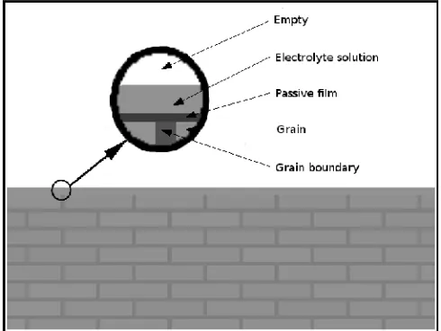
Each cell can assume N possible occupation states: E (empty), S (electrolyte), G (metal grain), B (grain boundary), P (corrosion product), and L (surface layer). The model has four parameters: Pmin, Pmax, Pbound, Player. Of those, Pmin and Pmax define the range of probabilities for the grain boundary (B) to corrode if it is in contact with a grain (G), Pbound is a probability for the grain boundary (B) not in contact with grain (G) to corrode, and Player is a probability for the corrosion of a surface layer (L).
[image:5.612.174.419.509.693.2]Initially, the lattice is subdivided into metal domain and solution domain (see Figure 1). The metal domain consists of a number of grains (G) separated by boundaries (B). The metal domain is bounded by a thin surface layer (L) and a thin solution layer (S). Remaining sites in the solution domain are marked as empty (E). Each grain is initially assigned a random probability Pgrain in the range between Pmin and Pmax. The value of Pgrain is uniform for the whole grain.
Figure 2. Moore neighbourhood of range 1.
The neighbours of each cell are those which belong to the Moore neighbourhood of range 1, as depicted in Figure 2. At each discrete time step there are the following events:
1. If B is in contact with at least one S and one G, it changes to S with probability Pgrain, corresponding to the G site.
2. If B is in contact with at least one S but not in contact with G, it changes to S with probability Pbound.
3. If L is in contact with at least one S or P, it changes to S with probability
Player.
Note, that in the model without diffusion sites of type E, S, G remain intact, and sites of type P are absent.
In the case of diffusion the CA rules are the following:
1. If B is in contact with at least one S and one G, it changes to S with probability Pgrain, corresponding to the G site.
2. If B is in contact with at least one S but not in contact with G, it changes to S with probability Pbound.
3. If L is in contact with at least one S or P, it changes to S with probability
Player.
The only difference in these rules compared to the case without diffusion is that S in rules (1) and (2) is changed to (P), i.e. metal changes to the corrosion product instead of transforming directly to the electrolyte solution.
After applying CA rules, diffusion is modelled by a random walk process. Potential walkers are the corrosion product sites (P), which are allowed to walk into neighbouring sites either occupied by electrolyte (S) or being empty (E).
The sites are chosen in random order. If the selected site is of type P, its random neighbour is selected. Then the options are as follows:
2. If the selected neighbour is E, it remains unaltered, and the current P site becomes S.
3. If the selected neighbour is neither S nor E, no changes are made.
The result mimics the diffusion of P species in the electrolyte E. The precise meaning of the concentration of P depends upon the parameters of the real system, for example, the concentration of any anion or cation.
3. SIMULATION RESULTS AND COMPARISON WITH EXPERIMENT
The simulation using the CA model described above was undertaken on a 640x320 lattice. Initially, there were 8x16=128 rectangular grains, each having size 76x16 cells, and the width of the grain boundary was set to 4 cells. The following values of the probability parameters were used: Pmin = 0.1, Pmax = 1.0, Pbound = 0.01,
Player = 0.0001. Thus, the probabilities of corrosion of the grain boundary cells adjacent to grains were uniformly distributed in the interval (0.1 – 1.0), and were greater than the probability Pbound. The value of Player was chosen to be small to ensure that the corrosion was not at the same time in different grain boundaries, but with random delay.
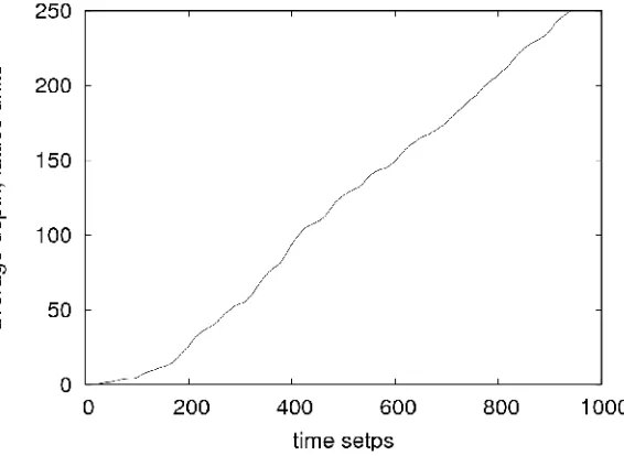
[image:7.612.158.441.420.627.2]The simulation runs were performed with disabled random walks, corresponding to the case without diffusion, and with enabled random walks, which simulate diffusion processes. The average depth of corrosion as a function of time is plotted in Figures 3 and 4. The time dependence is manifestly different without and with the effect of diffusion, tending to linear at large times in the former case, while noticeably slowing down in the latter case.
Figure 4. Corrosion propagation with diffusion.
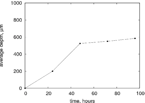
[image:8.612.133.462.317.639.2]Figure 6. Time dependence of the average depth of intergranular damage in the experiment (see Figure 5).
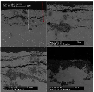
To compare the qualitative behaviour of the propagation of the intergranular corrosion, the average depth of corrosion was measured in the aluminium alloy Al 2024 T351 after immersion into sodium chloride and hydrogen peroxide solution. Figure 5 shows Scanning Electron Microscopic images at various immersion time periods. Figure 6 shows the average depth of inter-granular attack versus time. The qualitative behaviour of the time dependence of the average corrosion depth suggests that the model which includes diffusion is more appropriate for predicting the advance of intergranular corrosion.
4. CONCLUSION
In this paper we have developed a cellular automaton model for intergranular corrosion. The model is based on the set of CA rules in conjunction with random walk process, and has four adjustable parameters. The simulation results show qualitative agreement with experimental data on the advance of the corrosion front.
The model can be extended in several directions. The set of CA rules can be modified to include wider range of the electrochemical phenomena occurring in the process of intergranular corrosion in given materials. The parameters of the model can be tuned to the match specific experimental situations, which may allow a prediction of the propagation of the corrosion front for given conditions.
ACKNOWLEDGEMENTS
References
1. Vargel, C. 2004. Corrosion of Aluminium. Elsevier Science.
2. Von Neumann, J. and A. W. Burks. 1966 Theory of self-reproducing automata. Urbana : University of Illinois Press.
3. Meakin, P., T. Jøssang, and J. Feder. 1993. “Simple passivation and depassivation model for pitting corrosion,” Phys. Rev. E, 48(4):2906–2916. 4. Reigada, R., F. Sagus, and J. M. Costa. 1994. “A Monte Carlo simulation of
localized corrosion,” J. Chem. Phys., 101(3):2329–2337.
5. Gobron, S. and Ch. Norishige. 1999. “3D surface cellular automata and their ap- plications,” J. Visual. Comput. Animat., 10:143–158.
6. Johnsen, T., A. Jøssang, T. Jøssang, and P. Meakin. 1997. “An experimental study of the quasi-two-dimensional corrosion of aluminum foils and a comparison with two-dimensional computer simulations,” Phys. A, 242(3– 4):356–376.
7. Córdoba-Torres, P., R. P. Nogueira, L. de Miranda, L. Brenig, J. Wallen born, and V. Fairén. 2001. “Cellular automaton simulation of a simple corrosion mechanism: mesoscopic heterogeneity versus macroscopic homogeneity,” Electrochim. Acta, 46:2975–2989.
8. Córdoba-Torres, P., R. P. Nogueira, and V. Fairén. 2002. “Forecasting interface roughness from kinetic parameters of corrosion mechanisms,” J. Electroanal. Chem., 529:109–123.
9. Córdoba-Torres, P., R. P. Nogueira, and V. Fairén. 2003. “Fractional reaction order kinetics in electrochemical systems involving single-reactant, biomolecular desorption reactions,” J. Electroanal. Chem., 560:25–33. 10. Córdoba-Torres, P., K. Bar-Eli, and V. Fairén. 2004. “Non-diffusive spatial
segre- gation of surface reactants in corrosion simultions,” J. Electroanal. Chem., 571:189–200.
11. Saunier, J., A. Chaussé, J. Stafiej, and J. P. Badiali. 2004. “Simulations of diffu- sion limited corrosion at the metal―environment interface,” J. Electroanal. Chem., 563:239–247.
12. Vautrin-Ul, C., A. Chaussé, J. Stafiej, and J. P. Badiali. 2004. “Numerical simulations of corrosion processes. properties of the corrosion front and the formation of islands,” Cond. Mat. Phys., 4(40):813–828.
13. Taleb, A., A. Chaussé, Dymitrowska M., J. Stafiej, and J. P. Badiali. 2004. “Simulations of corrosion and passivation phenomena: Diffusion feedback on the corrosion rate,” J. Phys. Chem., 208:952–958.
14. Vautrin-Ul, C., A. Chaussé, J. Stafiej, and J. P. Badiali. 2004. “Simulations of corrosion processes with spontaneous separation of cathodic and anodic reaction zones,” Pol. J. Chem., 78(9):1795–1810.
15. Malki, B. and B. Baroux. 2005. “Computer simulation of corrosion pit growth,” Corrosion Sci., 47:171–182.
16. Saunier, J., Dymitrowska M., A. Chaussé, J. Stafiej, and J. P. Badiali. 2005. “Diffusion, interactions and universal behavior in a corrosion growth model,” J. Electroanal. Chem., 582:267–273.
17. Pidaparti, R. M., M. J. Palakal, and L. Fang. 2005. “Cellular automata approach to aircraft corrosion growth,” Int. J. Artificial Intelligence Tools,