JOURNAL OF FOREST SCIENCE, 58, 2012 (9): 381–390
Efficiency of adaptive cluster sampling and traditional
sampling for coastal mangrove in Hainan of China
Y. Lei
1, J. Shi
2, T. Zhao
31Research Institute of Resource Information and Techniques, Chinese Academy of Forestry, Beijing, China
2Academy of Forest Inventory and Planning, State Forestry Administration, Beijing, China
3School of Information Science and Technology, Beijing Forestry University, Beijing, China
ABSTRACT: Based on two species of Coastal Mangrove in Hainan of China, Sonneratia Apetala Buch-Ham and Sonneratia caseoli, we estimated the density of the two species to evaluate the efficiency of adaptive cluster sampling (ACS), simple random sampling (SRS) and traditional systematic sampling (SYS). Our initial experimental designs for ACS consisted of 5 unit areas, 6 initial sampling proportions, 4 initial sample sizes and 5 criterion values in 1,000 rep-etitions. From the aspect of factors influencing efficiency, we analysed the efficiency of ACS in various designs. We also compared the efficiencies of the three methods on the indexes of the relative error, the variance of density estima-tor and the relative sampling efficiencies. We found that ACS yielded smaller variance than the traditional sampling methods. ACS was a powerful sampling method when a population was spatially aggregated. We also determined the optimum unit area for the two species studied using the two estimators (HT and HH) of adaptive cluster sampling. They were 20 m2 (2 × 10 m), 15 m2 (3 × 5 m) for S. Apetala Buch-Ham and 25 m2 (5 × 5 m), 15 m2 (3 × 5 m) for S.
caseolari, respectively.
Keywords: adaptive cluster sampling; Horvitz-Thompson estimator; Hansen-Hurwitz estimator; simple random sampling; systematic sampling
The mangroves, known as a long-term adapta-tion to tidal and flood impacts and the tropical, subtropical coastal shelterbelt, have a huge role in disaster reduction. Studies of mangroves, including tall trees and low shrubs, face significant sampling challenges for sustainable resource management, monitoring and assessments. Previous attempts to estimate the distribution and abundance of man-groves have used a variety of techniques, each with its own underlying assumptions, biases, and limitations. Sampling mangroves may often pro-duce estimation problems because of the rarity and patchy distribution of many species of mangroves.
The problems are that many sampling units contain zero plant detections, and some sampling designs become highly inefficient because little informa-tion is provided on the species.
Adaptive cluster sampling (ACS) first proposed by Thompson (1990) can provide more efficient estimates and higher rates of encountering rare and clustered distribution species than compara-ble traditional sampling designs (Brown, Manly 1998; Smith et al. 2004). ACS allows the inclusion of additional sampling units (e.g. quadrats) in the immediate neighbourhood of any quadrat in which the target species is found. Thompson (1990) also
proposed the modified unbiased estimators such as Horvitz-Thompson (HT) and Hansen-Hurwitz (HH) for ACS. The advantages of ACS over tra-ditional sampling designs such as simple random sampling (SRS) and systematic sampling (SYS) are believed to be twofold: (1) an increase in sampling efficiency resulting in more precise estimates of population parameters, and (2) an increase in the number of observations of the target species may result in more reliable estimates of other popula-tion parameters such as species richness and com-position, and relative abundance. These advantages should be pronounced especially for rare and clus-tered populations such as mangroves.
ACS is often used in some research areas in which the number of targets is of natural distribution but is difficult to determine. The research on the appli-cation of ACS develops rapidly, and has been used increasingly in many fields such as biological envi-ronment, forestry and fishery survey. Brown (1994) surveyed some biological species by ACS, mainly including the patchy distribution of rare plants and the number of tree species. Philippi (2005) used the ACS to estimate the abundance of low density plant population within a local area. He compared the ACS sampling efficiency in 1 m2 and 4 m2 of the different area of sampling unit, and compared the estimation precision of HH and HT. The conclusion was that the variance of HT estimation was less than
HH; the estimation results in 1 m2 and 4 m2 of the initial sampling units were both reasonable. Many scholars believe that the ACS yields good results in the surveying of forest resources, particularly in the cluster and patchy distribution of the population (Roesch 1993; Smith et al. 1995). Magnussen et al. (2005) simulated the sampling efficiency of eigh-teen artificial spatial populations of deforestation polygons with each 200 × 200 km2 using ACS and
SRS designs, and the result was that the sampling er-ror of ACS was 30% lower than that of SRS.
Although many scholars carried out relevant researches on the ACS method, and made some case studies, their researches were usually a com-parison between the results of ACS technology and traditional sampling only under certain conditions (such as one or two fixed unit areas) (Roesch 1993; Smith et al. 1995; Magnussen et al. 2005; Philip-pi 2005). For ACS, different initial sample sizes, unit areas and criterion values (C) will all affect the results of estimation. Therefore it is necessary to further conduct the estimation effects in a variety of sampling designs, and then to obtain more ef-ficient ACS designs and summarize the evolution of sampling results. The content of the research presented here is to take the coastal mangroves for the study area from Hainan Province of south-ern China, simulate the sampling of two mangrove coastal species Sonneratia Apetala Buch-Ham and
Sonneratia caseolari based on the real distribution
data in the investigated area, and to estimate the density for evaluating the efficiency of ACS, SYS and SRS designs.
MATERIAL AND METHODS
Study area
[image:2.595.71.504.559.759.2]The Dongzhaigang Mangrove Natural Reserve is located in the northeast of Hainan Province, 32 km from Haikou (Fig. 1). The geographic coor-dinates are 19°38'–20°01'N and 110°34'–110°38'E. The altitude is about 10–80 m a.s.l., with gradient 3–7°. The terrain is high in the north and low in the south. The reserved areas are located in the northern fringe of a tropical monsoon climate. The
average annual temperature is 17.1°C, the highest temperature is 37.51°C and the lowest tempera-ture is 3°C. The average annual sunshine is 2,200 h; the average annual rainfall 1,700–1,933 mm, more than 80% concentrated in May–October. All these climatic and geographic factors undoubtedly had a significant effect on the types of species composi-tion of the mangrove family.
The reserved areas, with a lot of rare plants, are the mangrove provenance base, where there are
S. Buch-Ham, S. caseolari, Bruguiera sexangula,
B. gymnor-rhiza, B. s. var. rhynochopetala, Rhizophora stylosa,
Ceriops tagal, Kandelia candel and so on.
Six plots of different sizes were established us-ing typical samplus-ing because the mangrove spe-cies are distributed at the Hegang village in Haikou Dongzhaigang Mangrove Natural Reserve on the coast of the Qiongzhou channel, where S. Apetala
Buch-Ham, S. caseolaris and Kandelia candel
com-munities are present. Finally one of the plots was selected for simulation sampling designs consider-ing its size is the largest one out of the six plots and its study area is 60 m × 100 m where is mostly
S. Apetala Buch-Ham and S. casolaris. The two tree
species are good species of mangrove forest and are naturally distributed in low salinity and muddy tidal flats. The height of S. Apetala Buch-Ham is generally about 10–15 m, diameter at breast height (DBH) is about 10–25 cm. S. casolaris height is about 5–8 m and DBH 4–15 cm.
Survey in the field
The trees were examined in the plot consisting of 60 quadrats (each 10 m × 10 m in size) distributed as adjacent grid in the mangrove community.
In order to measure the quadrat accurately, the ropes were pulled out along one side of the tidal flat, a pole was inserted at every 10-m interval, and taking the straight line of direction toward the mangrove forest by a compass where poles were set. Finally the borders of the plot were enclosed through benchmarking and by plastic ropes.
The origin was at the corner of each quadrat, through which two straight lines were perpendicu-lar to the axes (x-axis, y-axis). The trees were mea-sured, including locations, species name, height, DBH (by calliper), crown diameter (by tape), clear length (by a measuring rod) in each quadrat. Data on locations of S. Apetala Buch-Ham and S.
caseo-laris were extracted to use for a simulation study in
the experiment. The spatial distributions of inves-tigated trees are described in Fig. 2. The dots rep-resent plants as Fig. 2 shows the actual coordinates
x and y (in m) of S. Apetala Buch-Ham and S.
ca-seolaris which appear rare and in spatial clustered
distribution within the plot.
Adaptive cluster sampling
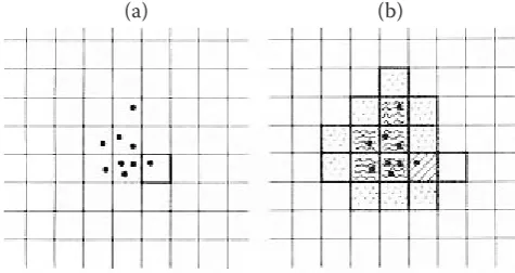
With an adaptive sampling scheme the procedure of selecting units to be included in the sample may depend on values of the variable of interest observed during the survey, i.e. the sampling is “adapted” to the data (Thompson 1990). ACS then operates under the rule that when the observed value of an initially sampled unit satisfies criterion conditions of interest (C), additional units in some pre-defined neighbourhoods will be added to the sample. Then, if any of these additional units satisfy C, the units in their neighbourhoods are added to the sample as well, and so on (Fig. 3). This process is iterated
0 20 40 60 80 100
0 10 20 30 40 50 60
x
y
(a)
0 20 40 60 80 100
0 10 20 30 40 50 60
x (b)
[image:3.595.67.525.556.713.2]y
until no units satisfying C are encountered (Turk, Borkowski 2005).
All neighbouring quadrats that collectively meet the criterion (e.g. y > 0) are called a network. The quadrats bordering each network that fail to meet the criterion are called edge quadrats. Network plus edge quadrats constitute the ACS cluster. Note that if any of the quadrats in a network is included in the initial random sample, the entire cluster will ultimately be included. In addition, it is important to note that any quadrat selected in the original sample that does not meet the criterion (i.e., y = 0) is considered a network of size 1. The grouping of quadrats into networks constitutes a partitioning of the initial population based on the size of the initial random sample.
Estimators
To estimate means and variances of interest, the modified Hansen-Hurwitz and Horvitz-Thompson estimators for ACS are described as follows.
A modified Hansen-Hurwitz type of estimator (HH)
According to Thompson (1990, 2002), an unbi-ased estimator of the population mean (ŷHH) formed by modifying the Hansen-Hurwitz estimate:
ŷHH= 1 n
∑
wi (1)n i=1
The variance of ŷHH is:
Var (ŷHH) = N – n n
∑
(wi – ŷHH)2 (2) Nn (N – 1) i=1where:
N – total number of sample units (quadrats) in the pop-ulation,
n – quadrats sampled,
wi –represents the average of the observations in the i-th network, define wi= yi/xi, xi – number of units in the i-th network, yi – observation values of the i-th network.
A modified Horvitz-Thompson type of estimator (HT)
Thompson (1990) presented the modified Hor-vitz-Thompson estimator, taking full advantage of probability of three kinds of units’ network inclu-sion in the sample (initial sample units, initial sam-ple units’ neighbourhood units which satisfy C, and edge units).
ŷHT = 1 v
∑
yk (3)N k=1 ak
αk = 1 –
[
(
N – xk)/(
N)
]
(4)n n
αik = 1 –
[
(
N – xj)
+(
N – xk)
–(
N – xj – xk)
]
(5) n n n
(
nN
)
Var (ŷHT) = 1
[
v∑
∑
v yj yk(
αjk – 1)
]
(6)N 2 j=1 k≠j αjk αjαk
where:
ŷHT– an unbiased estimator of the population mean
using the modified Horvitz-Thompson estimate, v – number of distinct networks in the sample,
N – total number of sample units (quadrats) in the
population, n – quadrats sampled,
yk – observation values of the network that includes unit k, yj – observation values of the network that includes unit j, αk – probability of the K-th network inclusion in the
sample, i.e. partial inclusion probability,
αjk – probability that the initial sample contains at least one unit in each of the networks j and k.
Simulation
Simulation can be useful for evaluating sampling designs because it permits experimental compari-son across populations and designs (Brown 2003; Morrison et al. 2008). In practice, it is often
in-Fig. 3. ACS sampling procedure example with one clus-ter: (a) an initial sample unit and (b) cluster obtained by adding adaptively. The one initial quadrat is squared and indicated with diagonal stripes, additional quadrats within intersected network are indicated with wavy lines, and edge quadrats are stippled if the criterion condition (e.g. y > 0 tree in a quadrat)
[image:4.595.62.300.56.182.2]feasible to analytically derive the sampling distri-bution for estimators across a range of populations and designs. Simulation study makes it possible to evaluate the sampling distribution of estimators based on a lot of repeated samplings. Comparisons across multiple populations and a broad range of designs can result in robust recommendations (Morrison et al. 2008).
Sampling designs
According to the characteristic of the rare, ag-gregate population, and the result of the smallest relative error of density estimator in many repeti-tions, the least initial sampling fraction was 0.06. The smallest initial unit area was 2 × 5 m.
The quantity of units that could be selected in dif-ferent unit sizes was 600, 400, 300, 240 and 200. The network did not expand mainly when C increased to 4 or 5. As the C continued to increase, the initial population was close to that of SRS. So the largest criterion value was no more than 5. Thus, criterion values (Ca) were set to be 1, 2, 3, 4 and 5, respec-tively. When the value of a selected unit was equal to or higher than the criterion value (C > Ca), addi-tional unit cross-shaped neighbourhood would be added to the sample.
Selecting the amount of units consisted of sam-ples from a population. The results reckoned by dif-ferent samples were difdif-ferent and also differed from the true value. Thus, the simulated results obtained by the sample only once cannot confirm whether the sampling method is good or not. We should compare various sampling methods and as many repetitions as possible.
The relative errors of the mean density estimated by HH and HT were respectively smaller than 5% in different repetitions and unit areas designs. The mean density estimated was to be invariable as rep-etitions increased to 1,000. Sampling designs were as follows:
– The conditions that the initial sampling fraction and C were invariant: various unit areas impacting on efficiency were analysed and compared, and a regular pattern was obtained. Sampling was simu-lated using ACS in five types of unit area designs [10 m2 (2 × 5 m), 15 m2 (3 × 5 m), 20 m2 (2 × 10 m), 25 m2 (5 × 5 m), 30 m2 (3 × 10 m)] and six initial sampling fractions (6, 8, 10, 12, 14 and 16%). – Provided that the initial sample size and C were
invariant: sampling was also simulated using ACS in five types of unit area design [10 m2 (2 × 5 m), 15 m2 (3 × 5 m), 20 m2 (2 × 10 m), 25 m2 (5 × 5 m),
30 m2 (3 × 10 m)]. According to previous survey experience and considering that the final sample size has enlarged, the lowest limit of the initial sample size was 15 and four kinds of initial sample sizes were 15, 25, 35 and 45. The optimal unit area was obtained in which the sampling was the most efficient.
Evaluated indicators
The survey data were imported into the software SAMPLE (it can be downloaded at http://www. lsc.usgs.gov/aeb/davids/acs/) to simulate sampling. The sampling without replacement was replicated 1,000 times in the process. The shape of sample unit was square or rectangle, and neighbourhood was cross-shaped. To evaluate the performance of sampling designs, we used measures of design ef-ficiency such as the variance of density estimator, relative error of density estimator and the relative sampling efficiencies. The relative sampling effi-ciencies (RE) are the ratio of variance from a tradi-tional sampling design to variance from the candi-date design with the final sample size equal among the two designs. The final sample size is fixed for conventional designs, but is random in adaptive de-signs. Thus, for adaptive designs the expected sam-ple size was the average of final samsam-ple sizes over 1,000 simulations. The variance of density estima-tor (E(v)) and the relative error of density estimaestima-tor are other measures of efficiency and precision. The relevant formulas are as follows:
Density estimator and variance in the i times sampling are ui and vi(i =1, 2, …, n), respectively:
µi = N ŷHT, HH (7) A
where:
ŷHT, HH – estimated values of the population mean using HT and HH estimate method, respectively, N – total number of sample units in the population,
A – total study area.
E(ˆμi) =
n
∑
µi(8)
i=1 n
E(μˆi) expresses the mean density estimated in certain repetitions and n represents the number of repetitions.
The variance of estimator is:
386 J. FOR. SCI., 58, 2012 (9): 381–390 Then the variance of estimator in m times
repeti-tions is:
E(v) =
n
∑
var (ˆμ)(10)
i=1 n
The relative sampling efficiencies:
Efficency (ˆμ) = E–y(vi)/E ˆ
μi (vi) (11)
where:
ˆ
μ – estimated population mean using ACS,
E–y(vi) – variance of density estimated using the traditional methods in the same final sample size of ACS,
Eμˆ
i (vi) – ACS variance of density estimated. An effi-ciency > 1 indicates that ACS would be more
precise than SRS or SYS and an efficiency < 1 indicates that the reverse is true – that SRS or SYS would be more precise than ACS.
The formula of the relative error of density estimator:
6%
0 0.0001 0.0002 0.0003 0.0004 0.0005
10 15 20 25 30
Va
ria
nc
e E
(
v
)
c = 2 c = 3 c = 4 c = 1
c = 5 (a)
8%
0 0.0001 0.0002 0.0003 0.0004
10 15 20 25 30 (b)
10%
0 0.00005 0.0001 0.00015 0.0002 0.00025
10 15 20 25 30 (c)
12%
0 0.00005 0.0001 0.00015 0.0002
10 15 20 25 30 (d)
14%
0 0.00005 0.0001 0.00015 0.0002
10 15 20 25 30 Unit area
(e)
16%
0 0.00005
0.0001 0.00015
10 15 20 25 30 Unit area
(f)
Va
ria
nc
e E
(
v
)
Va
ria
nc
e E
(
v
)
Va
ria
nc
e E
(
v
)
Va
ria
nc
e E
(
v
)
Va
ria
nc
e E
(
v
[image:6.595.69.522.112.708.2])
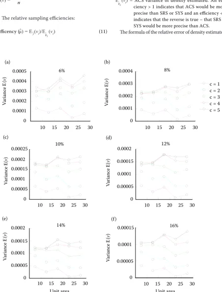
Fig. 4. The ACS variance in various unit areas, criterion values and initial sampling fractions for S. Apetala Buch-Ham
RESULTS AND DISCUSSION
Unit areas, initial sampling proportions and cri-terion values impacting on the variance
We would know that the HT and HH estima-tors of ACS for the mean relative errors of density estimated were 1.313 and 1.235% for S. Apetala
Buch-Ham and 2.082 and 1.95% for S. caseolari
in 6 initial sampling proportions and 5 unit areas when C were 1 to 5, which were all smaller than 5%. The difference between the density estimated and the real density was small, and the biggest rela-tive errors were 4.425% for S. Apetala Buch-Ham
and 4.446% for S. caseolari. The relative errors were much smaller for various unit areas. The HT and
HH estimators for the density variances were simi-lar in various simulation sampling designs. The HT
estimator of S. Apetala Buch-Ham, for instance, in-creased with the increase of C in a certain unit area and initial sampling fraction. The estimator vari-ance decreased as the unit area increased when C was 1. If C were 2 and 3, the estimator variances in various unit areas differed, while the trends were to decrease. When C was 4 or 5, the trends of variance were rising (Fig. 4).
For the results in Fig. 4, generally speaking, the smaller the C, the more units added to the sample. Thus the variances were smaller and the estimations were more accurate. Because of less units sampled, the variances increased as we increased C.
From general structures for further analysis, since the population is divided into different unit areas, the larger the unit area, the larger the unit value and the more easily a huge network could be
formed. Besides, the numbers of networks formed in both different unit areas and different C are dif-ferent. The larger the C, the more networks will be formed. Thus, for a certain unit area, when C is small, there are more units being included in the network and the larger networks are easily formed, while the size of a network would be smaller with the increase of C and the number of networks. The total variances of the population consist of the vari-ances within networks and the varivari-ances between networks. The variance within networks decreased as a result of the decrease of network size. This was to result in a smaller variance proportion of the to-tal variance in the network. The proportion of pop-ulation variance comprised of within network vari-ance might be the most important factor affecting sampling efficiency (Smith et al. 1995). For ACS, the greater the proportion of population variance comprised of within network variance was, the more efficient the sampling design was (Christ-man 1997, 2000; Brown 2003).
In a certain unit area, the proportion of population variance comprised of within network variance de-creased as the C values inde-creased, which inde-creased the sample variance too. In a certain C, with the increase of unit area, the proportion of population variance increased, but the variance decreased.
[image:7.595.64.530.598.708.2]The above factors influencing the sampling effect interacted and correlated. When C increased, the factors such as network size, proportion of popu-lation variance comprised of within network vari-ance and the amount of effective information in the sample, affecting ACS sampling effect were getting smaller and smaller, because the factor influenced
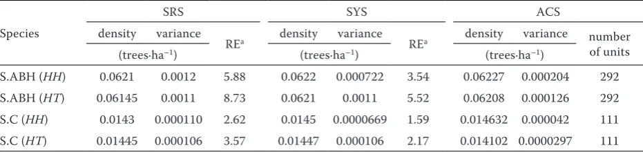
Table 1. Estimates and relative efficiency (RE) when C = 1 and the initial proportion and unit size were 6% and 10 m2
for the two species
Species
SRS SYS ACS
density variance
REa density variance REa density variance number
of units
(trees·ha–1) (trees·ha–1) (trees·ha–1)
S.ABH (HH) 0.0621 0.0012 5.88 0.0622 0.000722 3.54 0.06227 0.000204 292
S.ABH (HT) 0.06145 0.0011 8.73 0.0621 0.0011 5.52 0.06208 0.000126 292
S.C (HH) 0.0143 0.000110 2.62 0.0145 0.0000669 1.59 0.014632 0.000042 111
S.C (HT) 0.01445 0.000106 3.57 0.01447 0.000106 2.17 0.014102 0.0000297 111
SRS – simple random sampling, SYS – systematic sampling, ACS – adaptive cluster sampling, SABH (HH) or (HT) – esti-mates for Sonneratia Apetala Buch-Ham species using the HH or HT method, SC (HH) or (HT) – estimates for Sonneratia caseolari species using the HH or HT method, REa = Var
(SRS) /Var(ACS), REb = Var(SYS) /Var(ACS)
388 J. FOR. SCI., 58, 2012 (9): 381–390 by unit area was becoming lesser. As C was 4 or 5,
the range of factor variation and the effect on ACS sampling efficiency were reduced, and then the su-periority of ACS was not notable. The overall sur-vey for ACS was close to the traditional SRS. In a certain initial sampling proportion, the variance in-creased as the unit area inin-creased. This was because the initial sampling size decreased with the unit area increasing and the final efficiency information was getting less. According to each factor, its change rule and sampling results, we could conclude that when C was 1, the sampling efficiency was best based on the results (Fig. 3). So it was optimum for C = 1.
From simulation at a certain unit area, the mean
HH and HT estimators were both close to the real density in each initial sampling proportion, and there were no significant changes as initial sam-pling proportions increased, while the variances of density estimated by HH and HT decreased. The real density of S. Apetala Buch-Ham and S. caseo- lari was 0.0623 trees·ha–1 and 0.0145 trees·ha–1, respectively. Relative to HT, the amplitude of fluc-tuation for the results obtained by HH was smaller than HT and the density of HH was closer to the true value (Table 1). This result was similar to that of Talvitie et al. (2005).
For the two estimators (HT and HH), the vari-ance decreased as the initial sampling proportion
increased in a certain unit area and C (Fig. 4). But since HH estimator does not consider the prob-ability of the units included in the network, the in-fluence of network change on sampling result was weaker for HH than HT owing to different unit areas and C. Comparing HT with HH, the variance of HT
estimator was smaller when the unit area was large in a certain initial proportion and C. Table 1 shows the result of one design for the condition C = 1, the initial proportion and unit size were 6% and 10 m2. The variance of HT (0.000126) was smaller that of
HH (0.000204) for S.ABH (S. Apetala Buch-Ham).
Unit areas, initial sampling proportions and criterion values impacting on relative
efficiencies (RE)
Generally, ACS was compared with traditional sampling techniques by the relative efficiency pre-sented by Thompson and Seber (1996), the ratio of variance from traditional sampling method and ACS (e.g. variance of SRS divided by variance from ACS design). When the ratio was greater than 1, the efficiency of ACS was higher in the same final sample size. The relative efficiencies of ACS (HT
or HH) and the traditional methods were usually greater than 1 in various initial sampling
) a (
(c) (d)
HT estimator for S. Apetala Buch-Ham
0 0.01 0.02 0.03
Relative
erro
r
HH estimator for S. Apetala Buch-Ham
0 0.01 0.02 0.03
10 15 20 25 30
Re
la
tive err
or 15
25 35 45
HT estimator for S. caseolari
0 0.02 0.04 0.06
Unit area
Relative
error
HH estimator for S. caseolari
0 0.05 0.10
Unit area
Re
la
tive
erro
r
(b)
10 15 20 25 30 10 15 20 25 30
10 15 20 25 30
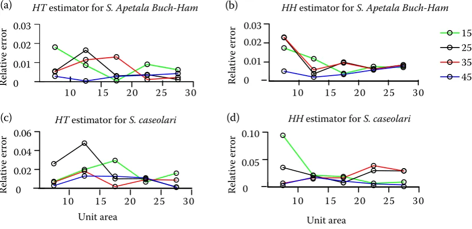
[image:8.595.62.524.448.672.2](a)
tions, unit areas and C. For example, REa > 1 and REb > 1 in Table 1. These indicated the efficiency of ACS was higher than SRS and SYS in the same final sample size of 292 and 111.
The efficiency of the traditional methods in-creased more quickly as the initial sampling pro-portions increased, while the superiority of ACS contributed more and more weakly. So it was ex-cellent to sample 6% initially from the population when ACS made full use of advantages relative to the traditional methods.
As for SYS and SRS in the same sample size, the efficiency of the former was higher when the sam-ple size was large. In a certain samsam-ple size, with the increase of unit area, the relative efficiency of SYS increased. In a certain unit area, along with the sample size reduced the relative efficiency of SYS was reduced. Therefore, SYS reached a higher rela-tive efficiency based on the larger sample size.
Reasonable unit areas in the same initial sample size
The design was conducted in the same initial sample size and repeated sampling 1,000 times when C was 1. The mean relative errors of HT and
HH were about 1% in four kinds of initial sample sizes (15, 15, 35 and 45).
We simulated several sampling efficiencies in dif-ferent unit areas and initial sampling sizes based on the relative errors of density estimation in four unit areas.
Fig. 5 shows that as the unit area increased, the relative errors of HH and HT presented roughly the same change rule. From the visual point of view, the unit area changed from 10 m2 to 15 m2 with greater relative error and variation of density. The relative errors and variations of density decreased with four initial sample sizes as the unit area increased.
As for HT estimation for S. Apetala Buch-Ham, the simulation sampling was perfect when the unit area was 20 m2 (Fig. 5a). As for HH estimation, when the unit area was 15 m2, the relative error was re-duced quickly (Fig. 5b). So the sampling effect was best when the unit area was 15 m2. That meant the relative error of density was larger when the unit area was smaller than 15 m2. While the unit area was larger than 15 m2, though the relative error was re-duced, the range of the relative error decreased too. And at the same time, with unit area increasing, the final sample size would increase significantly as well. That would lead to a higher sampling cost. Similarly,
for S. caseolaris, sampling was perfect when the unit
area was 25 m2 for HT estimation (Fig. 5c), while 15 m2 for HH estimation (Fig. 5d).
CONCLUSIONS AND SUGGESTIONS
The above analyses show that in a certain unit area, the initial sampling proportion and C, the variance of HT estimator is lower than that of the
HH estimator, and the variance of ACS is generally lower than that of SRS and SYS.
Density estimators using ACS are very close to the real values. The final sample sizes of SRS and SYS are the same as those of adaptive sampling (HH and HT
estimators). We know from the above analyses that: (i) ACS is more efficient than the traditional SRS and SYS and SYS is more efficient than SRS,
(ii) for the two estimators, the sampling efficien-cy based on the modified HT is greater than that based on the modified HH estimator.
In ACS designs, the variance estimated by the modified HT estimator is smaller usually than that estimated by the modified HH estimator. However, the modified HT estimator usually deviates from the real density more than the modified HH es-timator and this might be related to the network structure of population. For a population with dif-ferent network structure, the efficiency of each estimator should be studied further. At the same time, the modified HT estimator is usually more complex than the modified HH estimator. So in sampling designs or practical investigation appli-cations, we should choose a reasonable sampling estimator, not blindly pursuing minimum variance. With varied forms of neighbourhood, the neigh-bourhood’s form affects both the network size and the final sample size for ACS designs. And only the cross-shaped neighbourhood is used here. The neighbourhood of ACS impacting on the sampling efficiency can be further studied.
The uncertainty of the final sample size is one of the main existing problems for ACS. Although there has been some related research, the final sample size cannot be accurately predicted. Therefore, further re-search on controlling the final sample size of ACS is to be carried out. And how to cooperate the ground sampling technology and 3S techniques more closely with each other is also continued to be explored.
Acknowledgements
and software,also thank the two anonymous re-viewers for improving the scientific quality of this manuscript and the editors for their careful work.
References
Brown J.A. (1994): The application of adaptive cluster sam-pling to ecological studies. In: Fletcher D.J., Manly B.F.J. (eds): Statistics in Ecology and Environmental Monitoring. Dunedin, University of Otago Press: 86–97.
Brown J.A. (2003): Designing an efficient adaptive cluster sample. Environmental and Ecological Statistics, 10: 95–105.
Christman M.C. (1997): Efficiency of some sampling de-signs for spatially clustered populations. Environmetrics, 8: 145–166.
Christman M.C. (2000): A review of quadrat-based sam-pling of rare geographically clustered populations. Journal of Agricultural, Biological, and Environmental Statistics, 5: 168–201.
Magnussen S., Kurz W., Leckie D.G. (2005): Adaptive cluster sampling for estimation of deforestation rates. European Journal Forest Research, 124: 207–220. Morrison L.W., Smith D.R., Nichols D.W., Young C.C.
(2008): Using computer simulations to evaluate sample
design: an example with the Missouri bladderpod. Popula-tion Ecology, 50: 417–425.
Philippi T. (2005): Adaptive cluster sampling for estimation of abundances within local populations of low-abundance plants. Ecology, 85: 1091–1100.
Roesch F.A.Jr. (1993): Adaptive cluster sampling for forest inventories. Forest Science, 39: 65–69.
Smith D.R., Conroy M.J., Brakhage D.H. (1995): Efficiency of adaptive cluster sampling for estimating density of win-tering waterfowl. Biometrics, 51: 777–788.
Talvitie M., Leino O., Holpainen M. (2005): Inventory of sparse forest populations using adaptive cluster sampling. Silva Fennica, 40: 101–108.
Thompson S.K. (1990): Adaptive cluster sampling. Journal of the American Statistical Society, 85: 1050–1059. Thompson S. K. (2002): Sampling. New York, John Wiley
and Sons: 400.
Thompson S.K., Seber G.A.F. (1996): Adaptive Sampling. New York, John Wiley and Sons: 265.
Turk P., Borkowski J.J. (2005): A review of adaptive cluster sampling. Environmental and Ecological Statistics, 12: 55–94.
Received for publication October 12, 2011 Accepted after corrections July 23, 2012
Corresponding author:
Dr. Yuancai Lei, Research Institute Resource Information and Techniques, Chinese Academy of Forestry, Beijing 100091, China