Local modes based free shape data partitioning

Local Modes-based Free-Shape Data Partitioning

Plamen Angelov,

Fellow

,

IEEE

and Xiaowei Gu

School of Computing and Communications,

Lancaster University Lancaster, LA1 4WA, UK {p.angelov,x.gu3}@lancaster.ac.uk

Abstract—In this paper, a new data partitioning algorithm,

named “local modes-based data partitioning”, is proposed. This algorithm is entirely data-driven and free from any user input and prior assumptions. It automatically derives the modes of the empirically observed density of the data samples and results in forming parameter-free data clouds. The identified focal points resemble Voroni tessellations. The proposed algorithm has two versions, namely, offline and evolving. The two versions are both able to work separately and start “from scratch”, they can also perform a hybrid. Numerical experiments demonstrate the validity of the proposed algorithm as a fully autonomous partitioning technique, and achieve better performance compared with alternative algorithms.

Keywords— data partitioning; evolving clustering; parameter-free; data cloud; data- driven.

I. INTRODUCTION

Clustering has long been considered as one of the most effective tools for recognizing the underlying patterns within the data. As a supervised machine learning method, clustering currently is a very hot topic in the field of data analytics.

Established clustering algorithms [1-6] require different kinds of user inputs. For instance, the k-means algorithm [2] requires the number of clusters to be known beforehand, the DBScan algorithm [4] requires the radius and the minimum number of data samples within the radius to be predefined, etc. Although, these algorithms can achieve relatively high accuracy, their performances heavily rely on the user- and problem-specific parameters, which require clear prior

knowledge. However, in most real cases, the prior knowledge is too limited for pre-defining the user input, which, in turn, influences the efficiency and accuracy of the clustering algorithms.

The concept of a data cloud was introduced in [7] as a collection of data samples entirely based on the mutual distribution and ensemble properties. Thus, data clouds are nonparametric and they do not have a specific shape. The data clouds directly represent the distribution of the observed data samples instead of giving some desirable/excepted (often, subjectively) pre-defined smooth functions. A number of focal points (not necessarily to be the centres or means of the data clouds) representing the modes of the data density. They attract the nearest data samples to them and then form data clouds

forming Voroni tessellations [8] in the data space.

In this paper, we propose a new, fully autonomous algorithm named local modes-based data partitioning. This novel algorithm is entirely driven by the observed data samples and their mutual distribution in the data space. It can automatically identify the focal points representing the main modes of the data pattern merely based on the empirically observed data samples and then uses them to form data clouds.

Thus, there is no need for any kind of user- or problem-specific parameters or assumptions.

This algorithm has two versions, i) offline and ii) evolving. The offline version is designed to partition the offline dataset while the evolving version is for streaming data processing. They have the ability of starting “from scratch”, thus, they can both work independently. While a hybrid between the two versions is also possible. In this paper, we will introduce the two versions of the proposed method as two independent algorithms without loss of generality.

The remainder of this paper is organised as follows. Section II describes the theoretical basis of the proposed algorithm. The offline and evolving versions are separately introduced in sections III and IV. Section V summarizes main procedures of the proposed algorithm and section VI presents the numerical experiments and a discussion. The paper is concluded by section VII.

II. THEORETICAL BASIS

In this paper, the theoretical basis of the proposed local modes-based data partitioning algorithm will be introduced.

Frist of all, let us assume the data set/stream in the Hilbert data space d

R as

  

x k  x x₁, ₂,...,xk



,

T ,1, , 2,..., ,

i xi xi xi d

x ,

1, 2,...,

i k indicates the time instance that the ith data sample arrives. To be more general and realistic, we assume that some data samples within the data set/stream repeat more than once, namely,  x_i x_j, i j. The set of unique data samples can be denoted as

 



₁, ₂,...,



k l k 

u u u u (u_i u_i,1,u_i,2,...,u_{i d,} _T,

   

u k  x k, 1 lk k) and the corresponding frequencies of

occurrence

 



₁, ₂,...,



k l k

f  f f f (

1

1 k l

i i

f







).

In the rest of this section, the main operators of the recently introduced Empirical Data Analytics (EDA) [9]-[12] and their

corresponding recursive expressions disclosing the ensemble properties of the observed data samples will be introduced. At the end, the well-known Chebyshev inequality and its new, simpler form within the EDA framework will be briefly presented. The most widely used Euclidean type of distance is used in this paper for derivation clarity, but we have to stress that, the proposed algorithm can work with various types of distance as well.

A. Cumulative proximity

The cumulative proximity



of a particular data sample i

x (i1, 2,...,k) is defined as the sum of square distances between this data sample to all other data samples existing in the data space [9],[10]:

 

2



2 2



1

k

k i i j i k k k

j

k X









    

x x x x μ μ (1)

where 2



_{, ,}



2

1

d

i j i l j l

l

x x



 





x x . μ_k is the mean of

 

k x

and X_k is the average scalar product, and they can be updated recursively as:

k 1 k₁ 1 k; _{1 1}

k

k  k



  

μ μ x μ x (2)

X_k k 1X_k1 1 _k 2; X_{1 1}2

k  k



  x  x (3)

B. Standardized eccentricity

Standardized eccentricity is a very important measure for anomaly/fault detection [11]. The standardized eccentricity



of x_i (i1, 2,...,k) is defined in [11] as:

 

 

 

2 1

2

1 1 1

2 2

1

k

i l

k i l

k i k k k

k j j l

j j l

k k           







x x x x

x x x

(4)

The sum of the cumulative proximity of

 

k

x can be expressed using μ_k and X_k instead [11],[12]:

 

2



2



1

2

k

k i k k

i

k X

 

 



x μ (5)

Combining equations (1) and (5), the recursive expression of the standardized eccentricity,



is expressed as follows:

 

2 2

1 i k ; 1, 2,...,

k i k k i k X       x μ x

μ (6)

C. Unimodal density

Unimodal density [12] is defined as the inverse of

standardized eccentricity



. The unimodal density D of the data sample x_i (i1, 2,...,k) is expressed as follows [12]:

 

 

 

 

1 1 2 2 1 2 1 k k j j

k i k i

k i i k

k k D k X           



x x x

x x μ

μ

(7)

D. Multimodal density

The multimodal density, MM

D of a specific unique data sample u_i (i1, 2,...,l_k) is a weighted sum of its unimodal density by the corresponding frequency f_i , expressed as [12]:

 

 

 

1 2 2 1 2 1 k k k j j

MM i i

k i l

k i _{i k}

j j k k f f D k f X         





x u

u _{u μ}

μ

(8)

E. Chebyshev inequality

The well-known Chebyshev inequality [13] describes the probability of the distance between a certain data sample x_i

and the mean value to be larger than n times the standard deviation, namely, “n



”. We introduced earlier a more elegant and general form of Chebyshev inequality in terms of

standardized eccentricity,



, expressed as [11]:

P



k

 

i 1 n2



1 1₂

n

 x     (9)

The inequality (9) can be applied to anomaly detection directly regardless of the distribution of data samples [11].

III. OFFLINE LOCAL MODE-BASED PARTITIONING

The proposed offline version of the local modes-based partitioning algorithm employs the multimodal density,

MM

D as the main operator. The main procedure of the offline algorithm is summarized as follows:

Stage 1: Identifying the global maximum

For every unique data sample within the dataset

 

k x , its

local density, L

 

k i

D u (i1, 2,...,l_k) can be calculated using the following equation:

 

 

 

2 2 2 i L k d L

k i i L

k i D f k     



x u x u

u (10)

where d is the average distance between the data samples of

 



2



2 1 2 2 k k i i k k d X k   



  x

μ (11) The unique data sample with the highest _DL _{is selected as} the reference sample in the ranked unique data samples set

 

*

k

u :

*(1)



 



1,2,..., arg max k L k j j l D  

u u (12)

where u*(1) is the unique data sample with the global maximum of the local density DL and assign u*r u*(1). If there are more than one maximum, choose any one of them to be *r

u .

Stage 2: Re-ordering the local density

Then, we find the unique data sample which is nearest to

*r

u . Assuming there are q unique data samples holding the smallest distance to *r

u at the same time, they all will be selected and put into

 

*

k

u together as _u*(2)_{, u}*(3)_,…,u*(q1)_,

and their order will be decided by their local density DLin descending order. Once the unique data samples are put into

 

*

k

u , they will be removed from

 

k u .

This process continues with the rest of the data samples remaining in

 

k

u , and the last unique data sample, u*(q1), in

 

*

k

u is used as the reference data sample (u*r u*(q1)) to find its closest unique data samples, and then put them into

 

*

k

u and remove from

 

k

u . By repeating this procedure till

 

u k becomes , we can finally get the ranked unique data samples, denoted as

  

u* _k = u*(1)|i1, 2,...,lk



and their corresponding ranked local density collection:



D_kL

 

u*





   

 



L *(1) _, L *(2) _,..., L *(lk)



k k k

D u D u D u .

Stage 3: Detecting all local maxima

At this stage, we need to derive all local maxima of the ranked local density



D_kL

 

u*



using the sign function:

 





 

 







 

 



 









 





 

 













* 1 *

* * 1

* 1 *

*( ) sgn sgn 1 sgn 1 max j j L L k k j j L L k k j j L L k k j L

IF D D

D D

AND D D

THEN is a local imum of D

           u u u u u u u (13)

where sgn

 

 is the sign function:

 

1 0

sgn 0 0

1 0 x x x x         . We

denote the set of the local maxima of _DL _{as the set}

 

**



** j _{| 1, 2,...,} *



k

k  j l

u u ( *

k k

l l ).

Stage 4: Forming data clouds

Each local maxima, ** i

u is then set as a focal point/prototype of a data cloud. All other data samples are then assigned to the nearest focal point (local maximum) forming data clouds according to the following rule:





** 





*

1,2,...,

arg min , j k

i

j l

cloud label d



 x u (14)

After all the data samples within

 

k

x are assigned to the

data clouds, the actual center (mean) μ_{k j,} and the standard deviation _{k j,} ( _{1, 2,...,} *

k

j l ) of each data cloud can be calculated. Then we consider the set of centers, μ_{k j,} ( _{1, 2,...,} *

k

j l ) of the data clouds as if this is our dataset and calculate their multimodal density, MM

D using equation (8). The respective frequency of each data cloud is determined based on the sum of frequencies of the unique data samples associated with it.

The centers μ_{k j,} ( _{1, 2,...,} *

k

j l , *

k k

l l ) are ranked again in

the same way as described in stages 1 and 2, denoted as

 

*

k μ

and the corresponding standard deviations

 

* k

 as well. Then, the set of centers

 

*

k

μ is filtered according to the following rule:    









   









 





* 1 * * 1 *

* *

, 2

; 1, 2,...,

j j j j

k k k k

k j

k

IF d

j l

THEN is deleted

   _  _  μ μ μ (15)

From the Chebyshev inequality (equation (5)) we can see

that



 

5



3

4 k i

P  x   , which means more than 3

4 of the data samples are expected to be within 2 from the mean.

After the filtering operation, the collection of the filtered

data cloud centers denoted as

 

**



** j _{| 1, 2,...,} **



k k

k  j l

μ μ

( ** *

k k

l l ) is obtained, and they are passed to stage 4 for another round of filtering until the data cloud centers do not change any more.

Finally, we can get the filtering result, re-named as

 

o k

μ ,

and use the

 

o k

IV. EVOLVING LOCAL MODE-BASED PARTITIONING

The evolving version of the proposed local modes-based data partitioning algorithm works with the eccentricity,



and

unimodal density, D of the streaming data. The evolving

algorithm has three stages as follows.

Stage 1: Identification of the evolving local modes

For each new data sample, denoted as x_k1, that arrives, the global μ_k and X_k are updated to μ_k1 and X_k1 firstly using equations (2) and (3).

After the unimodal densities of x_k1 and all the existing local modes, D_k1



x_k1



and D_k1

 

μ_{k i,} (i1, 2,...,C_k) are obtained using equation (7), the following condition [14] is checked to see whether x_k1 is associated with a new local mode:





 





 





1 1 1 ,

1

1 1 1 ,

1 1

max

min

1 k

k C

k k k k i

i

C

k k k k i

i

k k

IF D D

OR D D

THEN C C

  _ 

  _ 



 _ 

 

 

 _ 

 

 

 

x μ

x μ (16)

where we use C_k as the number of existing local modes at the

kth time instance.

If this condition is met, a new local mode is added in the data space (C_k1C_k1). On the contrary, if the condition is not satisfied, x_k1 is associated with the nearest existing local mode and C_k1C_k.

Assuming x_k1is assigned to the ith (i1, 2,...,C_k1) local modewhich is decided by equation (14), the support of the ith

local mode is updated as S_k_1,i S_{k i,} 1; μk i, and Xk i, are

updated to μ_k_1,iand Xk1,i using equations (2) and (3). For other local modes, their parameters stay the same for the next processing cycle.

Stage 2: Filtering main local modes

Once there are no new data samples available, the data clouds will automatically be formed based on the existing local modes as focal points or poles of attraction around which to form data clouds. However, because data clouds do not have specific shapes, they may overlap with each other, thus, the redundant local modes need to be removed first.

The filtering stage begins from the data cloud with the smallest support and ends with the one with the largest support. For each data cloud, we check the following principle according to the Chebyshev inequality using the standardized eccentricity (equation (9)) [11]:



 





 







, , , ,

k i k j o k j k i o

th th

IF OR

THEN Merge the i and j data clouds together

 μ   μ 

(17)

Here, we use _o 5 , which corresponds to 2 as described earlier. _{k i,}

 

μ_{k j,} and _{k j,}

 

μ_{k i,} are the

standardized eccentricities calculated per data cloud

expressed as follows (i j) [12]:

 









, ,

2 2

, , ,

2 2

, , , , , , ,

1

1

k p k q

k p k q k p

k p k p k p k q k q k p k p

S

S S X S

 

 

   

μ

μ μ

μ μ μ

(18)

where p q, i or j and pq.

If the principle in equation (17) is met, the two data clouds

merge:

, , ,

, ,

, , ,

, ,

, ,

, , ,

, ,

1

k k

k i j k i k i

k j k i

k i j k i k j

k i j k i j

k j k i

k i j k i k j

k i j k i j

C C

S S S

S S

S S

S S

X X X

S S





 



 

 



 _{ }



 _{ }

  

  



μ μ μ (19)

Stage 3: Forming data clouds

After the main local modes were filtered out, the output is generated. The remaining local modes, re-named as

 

o

k

μ ,

are used as the focal points/prototypes to build data clouds

using equation (14).

V. ALGORITHM SUMMARY

In this section, the overall procedure of the two versions (offline and evolving) of the proposed local modes-based partitioning algorithm are presented in the form of pseudo-code in two separate subsections.

A. Offline local modes-based partitioning algorithm

i. Calculate D_kL

 

u_i (i1, 2,...,l_k ) using eq. (10);

ii. Find the unique data sample *(1)

u with global maximum of _DL_{using eq. (12);}

iii. Send *(1)

u into

 

*

k

u and L

 

*(1)

k

D u into



L

 

*



k

D u

and delete *(1)

u from

 

k u ;

iv. *r  *(1)

u u ;

v.While

 

k 

u 

* Find the unique data sample(s) which is/are nearest to *r

u ;

* Send the data sample(s) and the corresponding DL

to

 

* k

u and



D_kL

 

u*



, respectively; * Delete these data sample(s) from

 

TABLEI.DATASET DESCRIPTION-PART 1

Dataset

Details Number of Data

Samples

Number of Clusters

Number of Attributes

G1a _{450 3 2}

G2b _{800 2 2}

WWc _{750 5 3}

a. _{Gaussian dataset 1;} b. _{Gaussian dataset 2;} c. _{Wrist-worn accelerometer dataset.}

* Set the latest element in

 

*

k u as *r

u ;

vi. End While

vii. Filter

 

* k

u and



D_kL

 

u*



using eq. (13) and obtain

 

**

k

u as focal points of the data clouds;

viii.While

 

o k

μ are not fixed

* Use the focal points to form the data clouds from

 

x _kusing eq. (14);

* Obtain the parameters

 

k

μ and

 

k

 of the data clouds;

* Calculate D_kMM

 

μ_j ( j1, 2,...,l_k*) using eq. (8); * Find the _μ*(1) _{with maximum D}MM _{using eq. (12);} * Send μ*(1) into

 

*

k

μ and DkMM

 

μ*(1) into

 



MM *



k

D μ and delete _μ*(1) _from

 

k μ ;

* μ*r μ*(1) ; * While

 

k 

μ 

- Find the element(s) of

 

k

μ which is/are nearest

to _μ*r_;

- Send the element(s) and the corresponding MM D into

 

*

k

μ ;

- Delete the element(s) from

 

k μ ;

- Set the latest element in

 

*

k

μ as _μ*r_; * End While

* Apply eq. (15) to filter

 

*

k

μ and obtain new focal

points

 

**

k

μ ;

*

   

o **

k  k

μ μ

ix.End While

x. Build the data clouds with

 

o k

μ using eq. (14).

B. Evolving local modes-based partitioning algorithm

i. While the new data sample x_k1 of the data stream is

available (or until interrupted) * If (k0) Then

-μ₁x₁ - C₁1; - S_1,11; - μ_1,1x₁; - X_1,1 x₁ 2; * Else

- Update μ_k and X_k to μ_k1 and X_k1using eqs.

(2) and (3);

- If (Condition (eq. (16)) is met) Then

1. C_k1C_k1; 2.

1

1, k 1 k C S _{ }  ; 3.

1

1, k 1

k C  k

μ x ;

4.

1

2 1, k 1

k C k

X 

  x  ;

- Else

1. Use eq. (14) to decide the ith local modes

1

k

x is assigned to;

2. Update μ_{k i,} and X_{k i,} to μ_k_1,i and Xk1,i usingeqs. (2) and (3);

3. S_k1,i S_{k i,} 1; - End If

* End If

ii. End While

iii. Whiledata clouds exhibit overlap

* If (Condition (eq. (17)) is met) Then

- merge the two overlapping data clouds into one using eq. (19);

* End If

iv. End While

v. Obtain

 

o k

μ from the remaining local modes;

vi. Build the data clouds with

 

o k

μ usingeq.(14).

VI. NUMERICAL EXAMPLES

In this section, a number of benchmark problems were considered to evaluate the performance of the proposed algorithm.

For better analysis, we also consider a number of performance measures:

1) Inp: the parameters that have to be predefined (user input);

2) NoC: number of clusters/data clouds in the processing results;

3) AvP: the average purity of the clusters/data clouds, but may disguise poor results [5];

4) MaP: the maximum cluster/data cloud purity [5]; 5) MiP: the minimum cluster/data cloud purity [5]; 6) T: the execution time (in seconds).

A. Evaluation of the offline version

TABLEIII.DATASET DESCRIPTION-PART 2

Dataset

Details Number of Data

Samples

Number of Clusters

Number of Attributes

G3a _{1200 4 2}

G4b _{1250 5 2}

Cc _{938 2 2}

[image:6.612.52.269.58.492.2]

a. _{Gaussian dataset 3;} b. _{Gaussian dataset 4;} c. _{Real climate dataset} TABEL II . Comparison between offline algorithms

Inp Data set

Measures

NoC AvP MaP MiP T

LMa

G1

3 0.9978 1.0000 0.9934 12.13

MS b 0.3 3 0.9911 1.0000 0.9740 0.02

0.4 3 0.9844 1.0000 0.9554 0.02

KM c 3 3 0.9978 1.0000 0.9934 0.17

LM

G2

2 0.9475 0.9661 0.9303 10.07

MS

5 4 0.9413 1.0000 0.7647 0.03

8 2 0.9325 0.9832 0.8914 0.03

KM 2 2 0.9475 0.9661 0.9303 0.14

LM

WW

5 0.9973 1.0000 0.9868 5.11

MS

10 5 0.9947 1.0000 0.9804 0.02

12 3 0.6000 1.0000 0.5000 0.02

KM 5 5 0.9973 1.0000 0.9868 0.14

a.

Local Modes-based Partitioning Algorithm; b.

Mean Shift Algorithm; c.

K-means Algorithm.

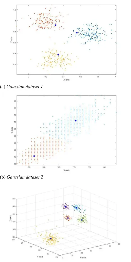
(a) Gaussian dataset 1

(b) Gaussian dataset 2

[image:6.612.307.563.71.305.2]

(c) Wrist-worn accelerometer dataset

Fig. 1 Offline partitioning results (Blue “*” stands for the focal points, if “” is in different colours, then it stands for different data clouds)

offline version of the proposed local modes-based partitioning algorithm on two synthetic Gaussian problems and a real problem (wrist-worn accelerometer dataset [15]) on a benchmark. The datasets used in the evaluation are tabulated in Table I. The partitioning results are presented in Fig. 1. The detailed experimental results are tabulated in Table II.

For further discussion of the performance, the offline version of the proposed algorithm is compared with two well-known offline clustering algorithms: mean shift [1] (needs the kernel size.



to be predefined) and k-means [2] (needs the number of clusters to be predefined). The experimental results of the two comparative algorithms are tabulated together in the Table II as well.

As we can see from Table II, the mean shift algorithm [1] is the fastest one from all the three, however, it is less accurate.

The k-means algorithm [2] is somehow comparable to the proposed local modes-based partitioning algorithm in terms of accuracy, but one has to keep in mind that the high accuracy of the k-means algorithm relies heavily on the properly pre-defined user input. In real cases, the number of clusters within a dataset is often hard to be decided because of the very limited

prior knowledge. Comparatively, the proposed algorithm is not

as fast as the other two algorithms, but it has the high accurate performance, and the most important point is that, it does not require any kind of user input.

B. Evaluation of the evolving version

[image:6.612.315.573.615.696.2]

[image:7.612.47.248.64.502.2]

TABEL IV . Comparison between evolving algorithms

Inp Data set

Measures

NoC AvP MaP MiP T

LM

G3

4 0.9958 1.0000 0.9900 2.00

DB a

0.06,

10 c 4 0.9325 1.0000 0.9965 0.10

0.08,

10 3 0.7350 1.0000 0.5017 0.16

ELMb 0.04 10 0.9967 1.0000 0.9870 1.06

0.06 3 0.7425 0.9802 0.5000 0.41

LM

G4

5 0.9920 1.0000 0.9689 2.24

DB

0.06,

10 5 0.9464 1.0000 0.9957 0.11

0.08,

10 3 0.5928 1.0000 0.3360 0.17

ELM

0.03 9 0.9912 1.0000 0.9689 1.18

0.04 6 0.8896 1.0000 0.6507 0.87

LM

C

2 0.9691 0.9747 0.9634 1.58

DB

1.6,

10 7 0.7985 1.0000 0.9966 0.04

2,10 3 0.8902 1.0000 0.9908 0.06

ELM

3 4 0.9670 1.0000 0.9592 0.42

5 3 0.6215 1.0000 0.5639 0.24

a. _{DBScan Algorithm;} b. _{ELM Algorithm;} c._{[Radius, minimum number].}

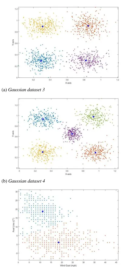
(a) Gaussian dataset 3

(b) Gaussian dataset 4

(c) Real climate dataset

Fig. 2 Evolving partitioning results (Blue “*” stands for the focal points; if “” is in different colours, then it stands for different data clouds)

The comparison results as depicted in Table IV demonstrate that, the proposed algorithm is the most accurate one of the three, and the most importantly, it is entirely data-driven and free from any pre-defined parameters or assumptions. In contrast, the DBScan algorithm is the fastest, but it is less accurate and needs two parameters to be decided by the user. ELM algorithm exhibits comparably accurate performance with the proposed algorithm; however, this also depends on the user input. With improperly defined radius, its performance can be significantly degraded.

C. Hybrid example between the offline and evolving versions

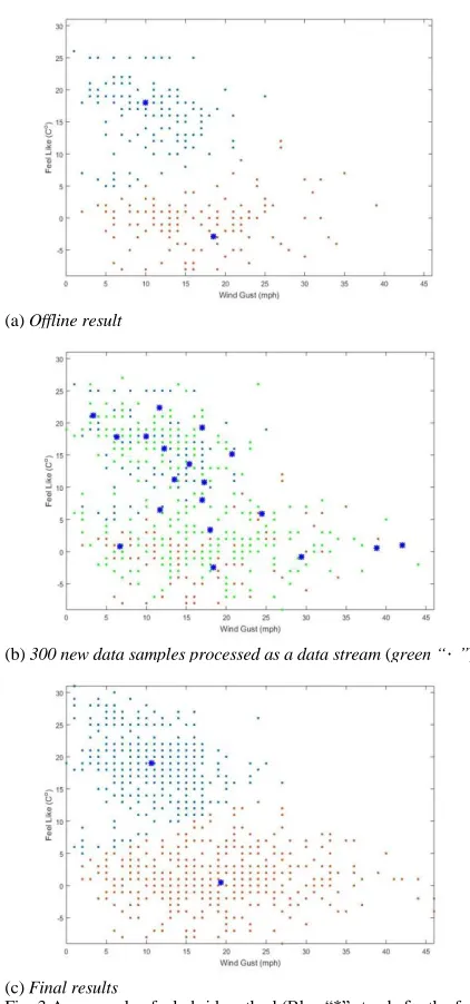
We use the same real climate dataset [16] as tabulated in Table II to study a hybrid between the offline version to start and the evolving version afterwards. The offline version is

applied to the first 300 data samples of the climate dataset [16] and the evolving version then is used to process the remaining 638 data samples as a data stream. The results of using the hybrid are shown in Fig. 3. From the figure we can see that the offline version builds two data clouds based on the 300 data samples. Then, the evolving version takes over the task and continues to process the rest of the data samples. The density changes with more data samples arriving and more clusters being formed based on the new data samples. Once, there are no anymore new data samples, the algorithm performs a filtering operation of the main modes and successfully identifies the two focal points representing the two main modes of the data density. Finally, the two focal points are used to form the two data clouds.

VII.CONCLUSION

In this paper, a novel “local modes-based” partitioning algorithm is introduced as a fully autonomous technique to partition the data space into parameter-free data clouds

[image:7.612.318.563.74.382.2] [image:7.612.314.564.83.374.2]

(a) Offline result

(b) 300 new data samples processed as a data stream (green “”)

[image:8.612.48.259.62.513.2]

(c) Final results

Fig. 3 An example of a hybrid method (Blue “*” stands for the focal points; if “”is in different colours, then it stands for different data clouds)

REFERENCES

[1] K. Fukunaga and L. Hostetler, “The estimation of the gradient of a density function, with applications in pattern recognition,” IEEE

Transactions on Information Theory, 1975, vol. 21, no. 1, pp. 32–40.

[2] J. B. MacQueen, “Some methods for classification and analysis of multivariate observations,” in Berkeley Symposium on Mathematical

Statistics and Probability, 1967, vol. 1, no. 233, pp. 281–297.

[3] S. L. Chiu, “Fuzzy model identification based on cluster estimation.,”

Journal of intelligent and Fuzzy systems, 1994, vol. 2, no. 3. pp. 267–

278.

[4] M. Ester, H. P. Kriegel, J. Sander, and X. Xu, “A density-based algorithm for discovering clusters in large spatial databases with noise,”

in International Conference on Knowledge Discovery and Data Mining,

1996, vol. 96, pp. 226–231.

[5] R. Dutta Baruah and P. Angelov, “Evolving local means method for clustering of streaming data,” in IEEE International Conference on

Fuzzy Systems, 2012, pp. 10–15.

[6] R. R. Yager and D. P. Filev, “Approximate clustering Via the mountain method,” IEEE Transactions on Systems, Man, and Cybernetics, vol. 24, no. 8, pp. 1279–1284, 1994.

[7] P. Angelov and R. Yager, “A new type of simplified fuzzy rule-based system,” International Journal of General Systems, vol. 41, no. 2, pp. 163–185, 2011.

[8] A. Okabe, B. Boots, K. Sugihara, and S. N. Chiu, Spatial tessellations: concepts and applications of Voronoi diagrams, 2nd ed. Chichester, England: John Wiley & Sons., 1999.

[9] P. Angelov, “Outside the box: an alternative data analytics framework,”

Journal of Automation, Mobile Robotics and Intelligent Systems, vol. 8,

no. 2, pp. 53–59, 2014.

[10] P. Angelov, “Typicality distribution function – a new density- based data analytics tool,” in IEEE International Joint Conference on Neural

Networks (IJCNN), 2015, pp. 1–8.

[11] P. P. Angelov, “Anomaly detection based on eccentricity analysis,” in

IEEE Symposium Series in Computational Intelligence, IEEE Symposium on Evolving and Autonomous Learning Systems, EALS, SSCI, 2014, pp. 1–8.

[12] P. P. Angelov, X. Gu, J. Principe, and D. Kangin, “Empirical data analysis - a new tool for data analytics,” in IEEE International

Conference on Systems, Man, and Cybernetics, 2016, p. in press.

[13] J. Saw, M. Yang, and T. Mo, “Chebyshev inequality with estimated mean and variance,” The American Statistician, 1984, vol. 38, no. 2, pp. 130–132.

[14] P. Angelov, Autonomous Learning Systems: From Data Streams to Knowledge in Real Time. John Willey, 2012.

[15] https://archive.ics.uci.edu/ml/datasets/Dataset+for+ADL+Recognition+ with+Wrist-worn+Accelerometer