Using
Publicly Available Data, Physiologically-Based
1Pharmacokinetic Model and Bayesian Simulation to Improve
2Arsenic Non-Cancer Dose-Response
3Zhaomin Donga,b, CuiXia Liub,c, Yanju Liua,b, Kaihong Yana,b, Kirk T. Sempled and Ravi Naidu*,a,b 4
5 a
Global Centre for Environmental Remediation, the Faculty of Science and Information Technology, 6
University of Newcastle, University Drive, Callaghan, NSW 2308, Australia 7
b
Cooperative Research Centre for Contamination Assessment and Remediation of the Environment 8
(CRC CARE), Mawson Lakes, SA 5095, Australia 9
c
School of Environmental Science and Engineering, Huazhong University of Science and Technology, 10
Wuhan 430074, China 11
d
Lancaster Environment Centre, Lancaster University, LA1 4YQ Lancaster, United Kingdom 12
13
* Corresponding Author: Ravi Naidu 14
15
ATC Building, Global Center for Environmental Remediation, Faculty of Science and Information 16
Technology, University of Newcastle, Callaghan, NSW 2308 17
Email: [email protected]
18
19
Contents
21
Abstract ... 3 22
Graphical Abstract ... 4 23
1. Introduction ... 5 24
2. Materials and Methods ... 6 25
2.1. Procedure for Establishing Arsenic Dose Response. ... 6 26
2.2. Exposure Assessment. ... 6 27
2.3. Biomonitoring Data. ... 7 28
2.4. PBPK Model. ... 8 29
2.5. Bayesian Simulation. ... 8 30
2.6. Dose-Response Assessment. ... 10 31
3. Results and Discussion ... 10 32
3.1. Exposure Estimation... 10 33
3.2. Urinary Arsenic Concentrations. ... 12 34
3.3. PBPK Model Optimisation. ... 13 35
3.4. Dose Response Assessment. ... 15 36
4. Limitations and Conclusions ... 16 37
5. Acknowledgements ... 17 38
6. Supplementary Materials Available ... 17 39
7. References ... 17 40
List of Tables ... 21 41
List of Figures. ... 25 42
Abstract
45
Publicly available data can potentially examine the relationship between environmental exposure
46
and public health, however, it has not yet been widely applied. Arsenic is of environmental
47
concern, and previous studies mathematically parameterized exposure duration to create a link
48
between duration of exposure and increase in risk. However, since the dose metric emerging from
49
exposure duration is not a linear or explicit variable, it is difficult to address the effects of exposure
50
duration simply by using mathematical functions. To relate cumulative dose metric to public health
51
requires a lifetime physiologically-based pharmacokinetic (PBPK) model, yet this model is not
52
available at a population level. In this study, the data from the U.S. total diet study (TDS,
53
2006-2011) was employed to assess exposure: daily dietary intakes for total arsenic (tAs) and
54
inorganic arsenic (iAs) were estimated to be 0.15 and 0.028 µg/kg/day, respectively. Meanwhile,
55
using National Health and Nutrition Examination Survey (NHANES, 2011-2012) data, the fraction
56
of urinary As(III) levels (geometric mean: 0.31 µg/L) in tAs (geometric mean: 7.75 µg/L) was
57
firstly reported to be approximately 4%. Together with Bayesian technique, the assessed exposure
58
and urinary As(III) concentration were input to successfully optimize a lifetime population PBPK
59
model. Finally, this optimized PBPK model was used to derive an oral reference dose (Rfd) of 0.8
60
µg/kg per day for iAs exposure. Our study also suggests the previous approach (by using
61
mathematical functions to account for exposure duration) may result in a conservative Rfd
62
estimation.
63
KEY WORDS: PBPK model; Dose response; Bayesian Simulation; Arsenic; Publicly
64
Available data
Graphical Abstract
66
TDS
NHANES
…
dose
re
sponse
1. Introduction
68
Chronic exposure to elevated levels of arsenic (As) has resulted in many adverse effects
69
appearing in humans (Maull et al. 2012; Naujokas et al. 2013). Epidemiological evidence
70
provides opportunities to undertake a dose-response study, and furthermore to assist in
71
assessment and management. For example, one study over a mean follow-up period of 9.7
72
years for 52,931 eligible participants suggested that the adjusted incidence rate ratios per 1
73
μg/L increment in arsenic levels in drinking water were 1.03 (95% confidence interval (CI):
74
1.01, 1.06) for all diabetes cases (Bräuner et al. 2014). Such epidemiological studies have
75
convincingly linked the As exposure level and risk (Bräuner et al. 2014; U.S. EPA 1988).
76 77
Excepting exposure level, previous research has also demonstrated the incidence of
78
diseases increases with exposure duration (Liao et al. 2008; Mazumder et al. 1998; U.S.
79
EPA 1988). To quantify the exposure duration effects, mathematical functions (such as
80
Weibull and Hill functions) have usually been employed, by parameterizing age factor to
81
represent exposure duration effect (Liao et al. 2008; U.S. EPA 1988). For long-term
82
chronic exposure, since the dose metric emerging from exposure duration is not a linear or
83
explicit variable, it is difficult to address these effects simply based on mathematical
84
parameterization (Hodgson and Darnton 2000; Philippe and Mansi 1998). The case study
85
on dioxin has successfully illustrated how to use toxicokinetic model to convert external
86
exposure level and exposure duration into a cumulative dose metric, which was further
87
applied in dose-response study (Becher et al. 1998; Crump et al. 2003). To understand the
88
influence of exposure duration to public health requires a toxicokinetic model to
89
appropriately quantify the impact of exposure duration on delivered dose and ultimately
90
risk in a quantitative dose-response framework.
91 92
Several toxicokinetic models have been previously developed (El-Masri and Kenyon 2008;
93
Liao et al. 2008; Yu 1999). Based on short-term oral exposures, Yu (1999) developed a
94
seven-compartment physiologically-based pharmacokinetic (PBPK) model for inorganic
95
As (iAs). More recently, El-Masri and Kenyon (2008) published an individual PBPK
96
model that traced the relationships among iAs, monomethylarsenic acid (MMA) and
97
dimethylarsenic acid (DMA) for oral exposure. While these models offered an overview of
98
the absorption, metabolism, distribution and excretion mechanisms in human systems, all
99
such models were developed based on normal people at an individual level. To relate
100
exposure to public health, a PBPK model needs to account for intrinsic heterogeneity at a
population and lifetime scale.
102 103
Publicly available data have the potential to support the optimization of population PBPK
104
models for use in quantitative risk assessment (Bernillon and Bois 2000; Lyons et al. 2008),
105
particularly in dose-response study. Specifically, the U.S. FDA has conducted a total diet
106
study (TDS) program to monitor the levels of multiple elements, as well as As, in the
107
country’s food supply (Tao and Michael Bolger 1999). Also, the National Health and
108
Nutrition Examination Survey (NHANES) program was initiated to assess the health and
109
nutritional status of adults and children in the United States (Aylward et al. 2014). Fitting of
110
PBPK models to available data using Bayesian methods such as Markov Chain Monte
111
Carlo (MCMC), these publicly available data can be utilized to bridge As exposure and
112
public health. To the best of our knowledge, this type of research has not previously been
113
attempted and represents a novel interpretation of human health from existing data sets.
114 115
In this study, the aim is to illustrate how to integrate publicly available data, PBPK model
116
and Bayesian simulation to refine human health risk assessment, using arsenic as a case
117
study. In particular, the objectives include: 1) assessment of As exposure from U.S. TDS; 2)
118
reporting As biomonitoring information based on the latest U.S. NHANES data
119
(2011-2012); 3) optimizing an As population lifetime PBPK model; and 4) improving As
120
non-cancer dose-response study. The newly proposed dose-response study has the potential
121
to protect human health from arsenic exposure.
122
2. Materials and Methods
123
2.1. Procedure for Establishing Arsenic Dose Response.
124
As shown in Figure 1, the procedure for establishing As dose response consisted of three
125
steps. In step 1, a national As exposure assessment was conducted based on TDS data. Then,
126
the urinary As data was retrieved from NHANES database. The As exposure information
127
and urinary As concentration were set as PBPK model input and output, respectively.
128
Therefore a population, lifetime PBPK model was optimized by using Bayesian simulation
129
(step 2). Finally, the optimized PBPK model assisted in As dose-response study (step 3).
130
131
2.2. Exposure Assessment.
132
The U.S. FDA has released analytical results for samples (all the samples in the TDS study
133
were table-ready prior to analysis) collected during 2006-2011 for toxic and nutritional
134
elements (U.S. FDA 2014). The total As concentrations (tAs) in 272 types of foods were
also measured. The foods were collected based on the food list representing the major
136
components of American people’s diet. In the meantime the U.S. FDA compiled food
137
consumption data from 9 age subgroups (U.S. FDA 2009). Therefore, the daily tAs
138
exposure (EAs) was estimated by multiplying arsenic concentration (CAs) and the 139
age-specific consumption amount (AAs) for each TDS food: 140
As As As
E =C ×A (1)
141
In this study, all 272 types of food were classified into six categories: seafood (exclude
142
fish), rice/bread/wheat, fish, vegetables, meat, wine and others.
143 144
Only tAs was available in the current TDS study. Lynch et al. (2014) have evaluated the
145
iAs fraction of tAs in food based on more than 6500 data points. To our knowledge, their
146
research is the most comprehensive available analysis on arsenic forms in food. Thus, the
147
fractions of iAs in different food categories were summarized in this study (Supplementary
148
Material(SM) Table S1), and were used to estimate daily exposure for different forms of As
149
in each food category.
150 151
Excepting diet exposure, drinking water was also deemed to be an important pathway for
152
iAs exposure. Xue et al. (2010) have estimated that the daily iAs exposure from drinking
153
water was 0.025±0.104 µg/kg.bw per day (median: 0.002 µg/kg.bw per day) for the U.S.
154
population. Consequently this median value was considered to be geometric mean (GM) of
155
drinking water exposure to help estimate arsenic exposure.
156 157
In this study, a log-normal distribution (LN) of daily intake was employed to account for
158
population variability:
159
As-Individual
E � LN GM GSD( , ) (2) 160
The median value of daily arsenic intake (the sum of dietary exposure and drinking water)
161
was used to represent the GM of this log-normal distribution, and the geometric standard
162
deviation (GSD) of iAs intake was estimated to be 1.58, which was based on a previous
163
survey of the general U.S. population (Yost et al. 2004).
164 165
2.3. Biomonitoring Data.
166
The urinary biomarker data, including the tAs, iAs, MMA, DMA, arsenobetaine and
167
arsenocholine was derived from the NHANES (n=4794) (NHANES 2014). The detection
168
rates for tAs, As(III), As(V), MMA, DMA, arsenobetaine, arsenocholine and
trimethylarsine oxide were 96%, 31%, 3%, 27%, 80%, 47%, 4% and 2%, respectively. A
170
log-normal distribution was assumed for urinary concentrations (Aylward et al. 2014), and
171
the maximum likelihood estimation (MLE) was performed to obtain the statistical
172
parameters, including the GM and GSD.
173 174
2.4. PBPK Model.
175
Our PBPK model was derived from previous studies (El-Masri and Kenyon 2008; Liao et
176
al. 2008; Yu 1999). Compared to prior models, this model allowed a lifetime exposure by
177
specifying some age-dependent parameters (Table 1). This human PBPK was a
178
five-compartment model consisting of four well-mixed tissue groups—liver, kidney, lung,
179
and rest of the body—and a mixed blood compartment (Figure 1). A detailed description of
180
the PBPK model and the programming code is available in the SM.
181
182
To account for the population variability of current lifetime PBPK model, three strategies
183
were used: firstly, the Gaussian distribution families were assumed for physiological
184
parameters (30% relative standard derivation (RSD) was used (Dong and Hu 2011), the
185
means of theses Gaussian distributions have been provided in Table 1); secondly, a
186
population optimization for sensitive parameters was performed based on a Bayesian
187
hierarchical model (BHM) (Lyons et al. 2008; Wan et al. 2013): to select the sensitive
188
parameters, a prior sensitivity analysis was carried out and the results were shown in Table
189
S2. Consequently, three parameters, i.e. liver/blood partition coefficients for As(III),
190
maximum metabolism rate constant for As(III)-MMA, urinary elimination constants for
191
As(III), were outlined as the sensitive parameters for optimization. Thirdly, a log-normal
192
distribution for daily exposure was adopted (as described in the earlier section).
193
194
2.5. Bayesian Simulation.
195
A BHM was established to estimate the sensitivity parameters as shown in Figure 1.
196
Predicted urinary levels (PULs) through the PBPK model by inputting the sensitive
197
parameters (Ps), exposure time (t) and other model parameters (Φ), and then PULs and
198
observed urinary levels (MULs) were linked through a residual error model (log-normal
199
distribution) with the mean (zero) and variance (σ2) in the likelihood calculation (Yang et al.
200
2010). Considering reported As exposure information did not distinguish the specifications
201
of organic arsenic (MMA, DMA, arsenobetaine and arsenocholine), correspondingly we
cannot employ the urinary organic arsenic (oAs) concentrations as the MULs in this study.
203
In contrast, we selected urinary As(III) levels as the MULs as the detection rate for As(V)
204
was too low (3%) to derive reliable statistics for As(V) (NHANES 2014).
205 206
Corresponding to Bayesian theory, the estimated posterior probability density function
207
(PPDF) for target parameters was obtained from the product of the joint prior probability
208
density function (pPDF) and the likelihood function. This was done based on the
209
measurement model describing the difference between the model simulation and the
210
observation (Lyons et al. 2008; Sohn et al. 2004). A joint prior probability distribution was
211
encoded asp(s2,Ps)= p(s2)×p P( s). Hence, the PPDF for s2andPs can be expressed by
212
Equation (3):
213
2 2
2 ,
( , s MULs) ( MULs s) ( s) ( )
Ps P C ∝ p C s P ×p P ×ps (3)
214
The prior distributions were non-informative for p(s2
) (a uniform distribution with
215
boundary of 0.001-100) and p(Ps) (normal distributions with 500% RSDs, the prior means
216
of these normal distributions have been noted in Table 1). With the prior distributions
217
forPsands2, the residual error model used in the likelihood function for different age
218
groups (i=1~6) was expressed as Equation (4):
219
n( MUTs i) n( ( s, , )) i n( PUTs i) i
L C − =L f P t Φ + =ε L C − +ε (4)
220
where εi was the error in age group i, which was termed 2
(0, )
i N
ε � s and f expressed
221
the PBPK model. With the prior distribution fors2
, the posterior distribution for the
222
parameters of interest was calculated by applying Equation (4) in the likelihood function
223
(Equation (5)):
224
6
2 , ,
1
( MULs s) ( MULs i PULs i s)
i
p C s P p C − C − P
=
∝
∏
(5)225
In this log-normal measurement model, 96 individuals (I) were chosen (Dong and Hu 2011)
226
due to the computational time required (approximate 90mins for each individual). MCMC
227
computation was used to optimize the parameters. The Gibbs and Metropolis Hastings (MH)
228
samplers were used to update the object parameters (Xu et al. 2006): 1) the parameter,s2,
229
was randomly drawn from the inverse gamma distribution by using the Gibbs sampler; 2)
230
the conditional distributions for Pshave no specific form as the PBPK model is non-linear, 231
and therefore we sampled the Ps by using the Metropolis algorithm. 232
2.6. Dose-Response Assessment.
234
Several symptoms have been considered to associate with ingested iAs (Bräuner et al. 2014;
235
Liao et al. 2008), while the skin lesions are considered as the most common symptoms.
236
Thus, the skin lesions of keratosis and hyperpigmentation were selected as the critical
237
non-cancer effects for As exposure in this study. Between April 1995 and March 1996, a
238
survey was conducted to investigate these two effects in West Bengal, India (Mazumder et
239
al. 1998). In all, 7683 participants were examined and interviewed, and the As levels in
240
drinking water were measured (Mazumder et al. 1998). The As levels and age were divided
241
into eight groups (0-50, 50-99, 100-149, 150-199, 200-349, 350-49, 500-799, and 800+
242
µg/L) and seven age groups (<9, 10-19, 20-29, 30-39, 40-49, 50-59, 60+), respectively
243
(Mazumder et al. 1998). Using the established PBPK model, drinking water iAs
244
concentration (Cw) was converted into urinary iAs concentration (UCiAs), and then
245
cumulative urinary concentration (CUC) was estimated by integrating UCiAs and age (t):
246
, , , w
(C )
iAs s
UC = f P Φt (6)
247
0
t iAs
CUC=
∫
UC dt (7)248
In our study, since previous studies indicated that the skin lesions were associated to
249
As-contaminated drinking water and drinking water was considered as major exposure
250
pathway (Bagla and Kaiser 1996; Mandal 1996; Mazumder et al. 1998), only drinking
251
water pathway was included when conducting dose-response study.
252 253
Then, the benchmark dose (BMD) approach was employed to estimate the iAs BMD and
254
the lower 95% confidence limit of BMD (BMDL) of the CUC (Davis et al. 2011; Wheeler
255
and Bailer 2009), and finally the BMDLCUC was extrapolated as the reference dose (Rfd).
256
To minimize model uncertainties, seven BMD models were included in this estimation,
257
including Gamma, Dichotomous-Hill, Logistic, Log-logistic, Probit, Logprobit and Weibull
258
models (Davis et al. 2011).
259
3. Results and Discussion
260
3.1. Exposure Estimation.
261
Of the 272 types of food, only the median value of 24 types were above the detection limit
262
(U.S. FDA 2014). Together with consumption data (U.S. FDA 2009), the median of daily
263
dietary tAs exposure was estimated to be 0.15 µg/kg/day (body weight was used as 70 kg).
264
Specifically, the values for age groups 0 - 0.5, 2, 6, 10, 14 - 16, 25 - 30, 40 - 45, 60 - 65, 70+
were 0.24, 0.39, 0.19, 0.18, 0.15, 0.16, 0.15, 0.20 and 0.16 µg/kg/day, respectively (Figure 2,
266
age-specific body weights as presented in Table 1 were used here). These age groups were
267
identical to the classification of age groups by U.S. Food and Drug Administration (U.S. FDA
268
2009). For young children (<6 years of age), the tAs exposure from food was approximately
269
1.5 - 2 times higher than that shown for other groups. Figure 2 also identified that the highest
270
contribution to tAs is made by seafood (58.46%, excluded fish), followed by rice/bread/wheat
271
(22.82%) and fish (14.72%).
272 273
The median value of estimated daily dietary iAs intake was 0.028 µg/kg/day for all age
274
groups. In particular the daily dietary intakes for As(III) and As(V) were estimated to be 0.020
275
and 0.0077 µg/kg/day, respectively. Thus, it was concluded that approximately 18.67% of tAs
276
exposure originating from diet was toxic iAs. Specifically, the iAs percentages for age groups
277
0 - 0.5, 2, 6, 10, 14 - 16, 25 - 30, 40 - 45, 60 - 65, 70+ were 40.67%, 27.56%, 27.37%, 21.34%,
278
22.19%, 21.44%, 19.43%, 12.76% and 12.38%, respectively. Thus, age differences were
279
observed (Figure 2): young children’s daily intake of iAs daily can be up to 0.11 µg/kg/day,
280
which was approximately 4 times higher than older age groups. However, the major
281
contribution to iAs exposure arose from rice/bread/wheat (84% for As(III) and 72% for
282
As(V)), while the rice/bread/wheat only contributed 23% to tAs exposure. Such differences
283
can be explained by the iAs fraction in food commodities (Table S1): although seafood made
284
the biggest contribution to tAs intake, the iAs fraction in seafood was approximately 1.2%.
285
Thus, seafood only contributed 3.66% and 5.38% for As(III) and As(V), respectively. On the
286
other hand, the fractions of As(III) and As(V) in the rice/bread/wheat were up to 49.01% and
287
15.99%, respectively.
288 289
Estimations in current study showed agreement with the urinary excretion: considering the
290
median value for tAs in urine for the general U.S. population was reported to be 8.15 µg/L
291
(Aylward et al. 2014), the daily intake should be approximately 12.68 µg/day. This is
292
assuming the urine volume is about 1.4 L per day and 90% of excretion was estimated by
293
urine (Pomroy et al. 1980): 8.15×1.4/90%=12.68 µg/day. Our dietary tAs exposure estimation
294
was 10.5 µg/day (0.15 µg/kg/day × 70 kg=10.5 µg/day), which is close to the total intake
295
amount of 12.68 µg/day. This estimation also indicated dietary is a major pathway, which has
296
been demonstrated in previous studies (MacIntosh et al. 1996; Yost et al. 2004).
297 298
Previous studies have reported daily arsenic exposure in the general U.S. population
(MacIntosh et al. 1997; Xue et al. 2010; Yost et al. 2004). For example, MacIntosh et al.
300
(1997) have reported that the mean dietary intake of tAs was 1.56 µg/kg/day (assuming an
301
adult weight of 70 kg), which was much higher than the median value (0.15 µg/kg/day) in this
302
report. Yost et al. (2004) estimated that for children the tAs exposure was 3.2 µg/day on
303
average, with a range of 1.6~6.2 µg/day, which was similar to the estimations in this study.
304
More recently, using data from 2003-2004 NHANES individual data, the median estimations
305
for tAs and iAs were 0.08 µg/kg/day and 0.02 µg/kg/day, respectively (Xue et al. 2010).
306
Comparing to the estimation for tAs in this study (median: 0.15 µg/kg/day), the estimation for
307
tAs was 2~3 times lower in the previous study (Xue et al. 2010).
308 309
Another difference between current study and the previous one is the contributions of food
310
commodities (Xue et al. 2010). One prior analysis showed that rice, wheat and related
311
products contributed about 29% of the iAs intake (Xue et al. 2010), which was much lower
312
than an estimation of 80.68% in this study. An estimation of only 24.32% iAs fraction in rice
313
(Schoof et al. 1999), which was adopt in previous study (Xue et al. 2010) and then resulted in
314
a low contribution being made by rice/bread/wheat. Contrastingly, a board array of literature
315
indicated that iAs fraction in rice was up to 65% (Jorhem et al. 2008; Lynch et al. 2014;
316
Torres-Escribano et al. 2008). Ancillary support provided by the European Food Safety
317
Authority also suggested that on average iAs represents approximately 70% of the tAs content
318
in rice, except for brown rice where on average iAs represents around 80% of tAs content
319
(EFSA 2014). Thus, previous report may underestimate the contribution of iAs from
320
rice/bread/wheat since it adopt a lower iAs fraction in rice/bread/wheat (Xue et al. 2010).
321 322
The iAs exposure from drinking water was estimated to be 0.002~0.004 µg/kg/day at a
323
national survey previously (Xue et al. 2010), which was referred to include drinking water to
324
calculate arsenic daily exposure in this study.
325
3.2. Urinary Arsenic Concentrations.
326
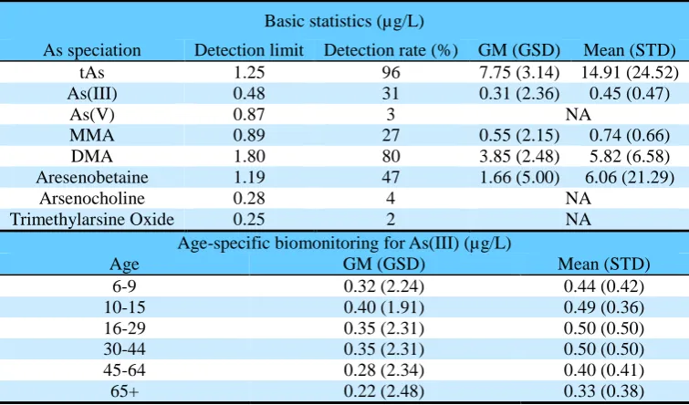
Of all the biomarkers examined for As exposure in the NHANES subjects (n=4794), the GM
327
and GSD were estimated to be 7.75 µg/L and 3.14, respectively (Table 2). Specifically, DMA
328
and arsenobetaine had relatively high concentrations, with GM of 3.85 µg/L and 1.66 µg/L,
329
respectively, followed by MMA (0.55 µg/L) and As(III) (0.36 µg/L). The age trend for As(III)
330
concentrations has also been statistically analysed (Table 2): the mean As(III) concentrations
331
for age groups 6-9, 10-15, 16-29, 30-44, 45-64 and 65+ were 0.44, 0.49, 0.50, 0.50, 0.40 and
332
0.33 µg/L, respectively.
334
This study marks the first one to document As(III) concentration in the general U.S.
335
population. For 2011-2012 NHANES data, the detection limit for As(III) declined sharply
336
from 1.2 µg/L (2009-2010 NHANES) to 0.48 µg/L (2011-2012 NHANES). Thus, the
337
detection rate increased from <5% to 31%, which provided an opportunity to estimate As(III)
338
concentration in general population. Based on a log-normal assumption for As(III), the As(III)
339
concentration using MLE methods was evaluated. A previous study stated that the MLE
340
method has an acceptable error ratio (0.7%), and further simulation indicated that only when
341
the detection rate fell below 25%, did the error ratio dose differ from zero (Croghan and
342
Egeghy 2003). In this study the impact of low detection rate was also simulated (Matlab
343
pseudocode is provided in the SM). The simulated results showed the error ratio was below
344
5% (detection rate>30%) when the size was 4794 (the population size in this study), which
345
suggested our estimated As(III) may be reliable.
346 347
Aylward et al. (2014) observed that the secondary methylation index (SMI, ratio of urinary
348
DMA to MMA) in the NHANES program likewise is much higher in people with measurable
349
arsenobetaine than in those without, suggesting that direct DMA exposure is co-occurring
350
with exposure to arsenobetaine. Such study indicated correlations among urinary DMA,
351
MMA, and arsenobetaine may potentially characterize source exposure (Aylward et al. 2014).
352
Figure 3(d) illustrates a relationship between DMA and MMA
353
(Ln(DMA)=1.04×Ln(MMA)+1.83, n=1280, p<0.0001), may indicate direct exposure to these
354
species in seafood or the metabolism of organic arsenicals. Previous analyses did not correlate
355
As(III) and organic arsenic at the national scale due to As(III) concentration was not available.
356
In this study, Figure 3(a)-(c) stated there were significant log-log linear regressions between
357
As(III) and tAs, MMA and DMA. The correlations between As(III) and MMA
358
(Ln(MMA)=0.55×Ln(As(III))+0.48; r2=0.35, n=944, p<0.001) were apparently more
359
significant than those between As(III) and DMA (Ln(DMA)= 0.87×Ln(As(III))+2.27; r2=0.27,
360
n=1480, p<0.001). This can be explained by the metabolism from MMA to DMA, which
361
would amplify the heterogeneities when addressing the relationship between As(III) and
362
DMA. Such heterogeneities were also propagated when linking As(III) and tAs, which would
363
reduce the fit (Figure 3(a), Ln(tAs)= 1.04×Ln(As3)+3.06; r2=0.19, n=1486, p<0.001). These
364
correlations may help trace arsenic exposure in the future.
365 366
3.3. PBPK Model Optimisation.
Although nine age groups were used in the TDS, the youngest participant in the NHANES
368
program was 6 years old. Therefore, the daily exposure estimations for the six age groups (as
369
listed in Table 2) were identical to average exposures of (6 yrs, 10 yrs), (10 yrs, 14-16 yrs),
370
(14-16 yrs, 25-30 yrs), (25-30 yrs, 40-45 yrs), (40-45 yrs, 60-65 yrs), and (60-65 yrs, 70 yrs),
371
respectively. The Gelman-Rubin diagnostic method served to test the convergence of the
372
objective parameters (Dong and Hu 2011) and was achieved in this study. The posterior
373
distribution for the three sensitive parameters, including the liver/blood partition coefficient
374
for As(III), maximum metabolism rate constant for As(III)-MMA, and the urinary elimination
375
constant for As(III), were estimated to be 20.93 ± 11.33 (95%CI: 0.95 - 41.19), 5.68×10⁻⁷ ±
376
2.85×10⁻⁷ (95%CI: 0.68×10⁻⁷- 1.12×10⁻⁶) mol/min and 0.098 ± 0.046 (95% CI: 0.019-0.19)
377
(min-1) (as shown in Table 1), respectively. Comparison with the prior value from previous
378
literature, increases of 26.79% and 9.23% were found for liver/blood partition coefficient and
379
maximum metabolism rate constant for As(III)-MMA, respectively. The increase for
380
liver/blood partition indicated the As(III) partitioned more in the liver, and the increase for
381
maximum metabolism rate constant suggested arsenic is more able to achieve maximum
382
metabolism. On another aspect, the posterior urinary elimination constant, a much higher with
383
a value of 40% increases (comparing to prior value), suggesting that As (III) was excreted
384
more readily in urine.
385 386
These parameter updates can be explained by the error between simulation results and
387
observed values (SM Figure S1). Using prior information, the simulated GM±GSD of As(III)
388
for the 6-9, 10-15, 16-29, 30-44, 45-64 and 65+ age groups were 0.19±1.91, 0.24±1.91,
389
0.41±1.86, 0.44±1.83, 0.39±1.85, 0.33±1.83 μg/L, respectively. The simulated concentrations
390
for 6-9 and 10-15 were 40% lower than the observed values, while those values for other
391
groups were 17%-50% higher than the observed values (corresponding As(III) levels, i.e.
392
0.32±2.24, 0.40±1.91, 0.35±2.31, 0.35±2.31, 0.28±2.34, 0.22±2.48 μg/L). By using the
393
posterior information, the simulated values (GM±GSD) of As(III) for the six age groups were
394
0.20±2.34, 0.24±2.29, 0.36±2.19, 0.38±2.14, 0.29±2.16, 0.23±2.13 μg/L, respectively.
395
Generally, the residual error was magnified with the cumulative probability increased due to
396
the positive skewness of the lognormal distribution. Although the relative differences between
397
the 6-9 and 10-15 age groups were still up to 0.38 and 0.40, the average difference for the
398
following four age groups fell to only 0.053, and the overall relative residual sum of squares
399
(RRSS) decreased from 0.85 to 0.31. Through Bayesian inference, crucial parameters in the
400
PBPK model were updated based on the prior distributions, further, calibration of the PBPK
model improved the prediction of biomonitoring data. Therefore, the updated parameters
402
under the constraints imposed by the model structure, model parameters, and the prior
403
exposure, represent more responsible population parameters that can be used to better
404
understand how exposure events are linked.
405 406
3.4. Dose Response Assessment.
407
The drinking water iAs concentration and age were inputted into the established PBPK model
408
to estimate CUC (Equations 4-5). The data for females and males subjects were combined
409
since the PBPK model did not treat the genders separately. Overall incidences of
410
hyperpigmentation and keratosis were 4.56% and 2.01%, respectively. Both types of skin
411
lesions demonstrated a positive age trend, as exemplified the hyperpigmentation incidences
412
for the age groups <9, 10-19, 20-29, 30-39, 40-49, 50-59, >60 were 1.83%, 2.31%, 4.14%,
413
5.90%, 7.21%, 9.10% and 7.5%, respectively.
414 415
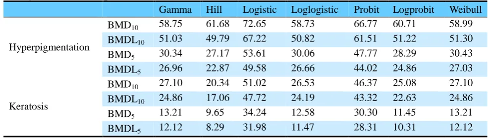
Table 3 showed the iAs BMD estimation for different models when BMR were set as 10%
416
and 5%. The estimated iAs BMDL10 ranked from 17.06 - 72.65 µg/kg per day, while the iAs
417
BMDL5 were estimated with a range of 8.29 - 46.37 µg/kg per day. Using the keratosis as the
418
critical effect and BMR of 5%, the PoD (Point of Departure) was estimated to be 8.29 µg/kg
419
per day (the lowest BMDL estimation was used). Since the data for dose-response was only
420
stemmed from one report, an uncertainty factor of 10 was considered to account for
421
population variability. Thus, the iAs Rfd was adjusted to be 0.8 µg/kg per day. As stated,
422
current diet iAs daily intake was estimated to be 0.028 µg/kg/day, which suggested the hazard
423
quotient (HQ) was only 0.035. Such a low HQ indicated an insignificant risk for skin lesions
424
when the general U.S. population was exposed to iAs.
425 426
Previous studies also functionally parameterized exposure duration to create a link between
427
risk increases and exposure duration (Liao et al. 2008; U.S. EPA 1988). Contrastingly, this
428
study used a PBPK model to include the impacts from exposure duration. For comparisons,
429
the dose-response data was also analysed using a generalized multistage function to
430
parameterize exposure duration (U.S. EPA 1988):
431
2
0 1
( , ) 1 exp( ( ( ) )k
p duration dose = − − k ×dose× duration k− (8)
432
where the parameters k0, k1, k2 were skin lesion-specific best-fitted parameters, and model 433
simulations were provided in SM Table S3, as well as risk-specific dose in SM Table S4.
Using a response (p in Equation 8) of 5%, the Rfd was estimated to be 0.40 µg/kg per day (for
435
hyperpigmentation) when considering the intra-specific UF of 10. Thus, our analysis suggests
436
the previous method may result in a conservative Rfd estimation, since one fold higher Rfd
437
was obtained when using PBPK model. Moreover, using PBPK model to convert age into a
438
dose metric not only took into account the cumulative effect, but also simplified the model fit
439
since it involved fewer variables. A non-straightforward fit will emerge if the models used to
440
fit dose-response model is too complicated. In fact the Weibull model (Liao et al. 2008), was
441
also attempted to parameterize the age-effect in our study, however, the simulated results did
442
not converge (data not shown).
443 444
Arsenic Rfd on humans from epidemiological data was previously evaluated by the U.S.
445
EPA’s IRIS (U.S. EPA 2012). Using the data from a Taiwanese farming population exposed to
446
arsenic in well water, a chronic RfD of 0.3 µg/kg/day for inorganic arsenic was derived, based
447
on a NOAEL of 0.8 µg/kg/day for skin effects and possible vascular complications. However,
448
the Taiwanese dose-response data is not publicly available currently, which make it is
449
impossible to implement the estimations and comparisons for this population group.
450
4. Limitations and Conclusions
451
Some limitations have been acknowledged in this study. The total exposures considered only diet
452
and drinking water, since it was difficult to trace other pathways. This treatment may bring the bias
453
since this value was used as input to optimise the PBPK model parameters. However, previous
454
studies have demonstrated that diet and drinking water were the major exposures, and such
455
estimations agree well with the biomonitoring in our analysis. Also, only As(III) was used for
456
fitting the model parameters and the biomonitoring information for MMA and DMA was discarded:
457
this modelling endeavour omits MMA and DMA. These arsenic species (MMA and DMA) have
458
been known to have high activity and are likely the causes of many of even most of arsenic
459
biological effects (Ahmad et al. 2002; Andrewes et al. 2003). This flaw resulted from that the
460
details of exposure information on oAs is not available currently. Since oAs is much less toxic than
461
the inorganic fraction, such a consideration may have limited impact on assessing toxicity. On
462
another aspect, while cancer may drive the usual arsenic risk assessments, only Rfd based on
463
non-cancer effect is estimated. This consideration is due to the dose-response data is available for
464
hyperpigmentation and keratosis, but the raw data for cancer effects cannot be accessed based on
465
our extensive literature review. Each of these limitations may result in some amount of error or
466
bias into our study, and more available data promises to overcome these limitations.
467
One major aim of this study is to illustrate how to employ publicly available data inform
469
environmental regulations. Toward the next generation (NexGen) of human health risk
470
assessment strategies, new technologies are being used to collect and organize data streams
471
that promise to reshape our understanding of chemical behaviour (Krewski et al. 2014). By
472
exchanging such data, more hypotheses, methods and conclusions could benefit both
473
researchers and stakeholders. For example, current publicly available datasets (such as
474
ACToR, NHANES, National Morbidity, Mortality, and Air Pollution Study, IRIS) have
475
largely advanced research on human exposure and health outcomes (Fowler 2013), especially
476
when examining the links between public health and exposure to a certain chemical as shown
477
in this study.
478 479
In conclusion, not only did we estimate dietary tAs and iAs exposures for the general U.S.
480
population, our study is also the first to report that the fraction of As(III) levels in total arsenic
481
was approximately 4%. Moreover, a population PBPK model was optimised to help derive
482
iAs Rfd of 0.8 µg/kg per day for skin lesions. The framework presented here illustrates how to
483
use publicly available data and computational techniques to help stakeholders make informed
484
decisions.
485
5. Acknowledgements
486
We would like to thank the Cooperative Research Centre for Contamination Assessment
487
and Remediation of the Environment (CRC CARE) for funding support, and the Global
488
Centre for Environmental Remediation, University of Newcastle for use of its facilities.
489
6. Supplementary Materials Available
490
Information describing the PBPK model, pseudocode for PBPK model, pseudocode to
491
address the impact of low detection rate, fractions of As(III) and As(V) in food, sensitivity
492
analysis results for PBPK parameters, model fit results, risk-specific dose under generalized
493
multistage function, contour of the residual error between the simulated urinary As levels and
494
the observed urinary As levels here are provided.
495
7. References
496
Ahmad S, Kitchin KT, Cullen WR. 2002. Plasmid DNA damage caused by methylated arsenicals, 497
ascorbic acid and human liver ferritin. Toxicol Lett 133:47-57. 498
Andrewes P, Kitchin KT, Wallace K. 2003. Dimethylarsine and trimethylarsine are potent genotoxins 499
in vitro. Chem Res Toxicol 16:994-1003. 500
Aylward LL, Ramasamy S, Hays SM, Schoeny R, Kirman CR. 2014. Evaluation of urinary speciated 501
Regul Toxicol Pharmacol 69:49-54. 503
Bagla P, Kaiser J. 1996. India's spreading health crisis draws global arsenic experts. Science 504
274:174-175. 505
Becher H, Steindorf K, Flesch-Janys D. 1998. Quantitative cancer risk assessment for dioxins using an 506
occupational cohort. Environ Health Perspect 106:663. 507
Benramdane L, Accominotti M, Fanton L, Malicier D, Vallon JJ. 1999. Arsenic speciation in human 508
organs following fatal arsenic trioxide poisoning - a case report. Clin Chem 45:301-306. 509
Bernillon P, Bois FY. 2000. Statistical issues in toxicokinetic modeling: A Bayesian perspective. 510
Environ Health Perspect 108:883-893. 511
Bräuner EV, Nordsborg RB, Andersen ZJ, Tjønneland A, Loft S, Raaschou-Nielsen O. 2014. 512
Long-term exposure to low-level arsenic in drinking water and diabetes incidence: A prospective 513
study of the diet, cancer and health cohort. Environ Health Perspect 122:1059. 514
Brown R, Delp M, Lindstedt S, Rhomberg L, Beliles R. 1997. Physiological parameter values for 515
physiologically based pharmacokinetic models. Toxicol Ind Health 13407:484. 516
Croghan C, Egeghy P. 2003. Methods of dealing with values below the limit of detection using SAS. 517
Southeastern SAS User Group, St Petersburg, FL:22-24. 518
Crump KS, Canady R, Kogevinas M. 2003. Meta-analysis of dioxin cancer dose response for three 519
occupational cohorts. Environ Health Perspect 111:681. 520
Davis JA, Gift JS, Zhao QJ. 2011. Introduction to benchmark dose methods and US EPA's benchmark 521
dose software (BMDS) version 2.1. 1. Toxicol Appl Pharmacol 254:181-191. 522
Dong Z, Hu J. 2011. Development of lead source-specific exposure standards based on aggregate 523
exposure assessment: Bayesian inversion from biomonitoring information to multipathway 524
exposure. Environ Sci Technol 46:1144-1152. 525
EFSA. 2014. Dietary exposure to inorganic arsenic in the European population. 526
El-Masri HA, Kenyon EM. 2008. Development of a human physiologically based pharmacokinetic 527
(PBPK) model for inorganic arsenic and its mono-and di-methylated metabolites. J 528
Pharmacokinet Pharmacodyn 35:31-68. 529
Fowler BA. 2013. Computational toxicology: Methods and applications for risk assessment:Academic 530
Press. 531
Hodgson JT, Darnton A. 2000. The quantitative risks of mesothelioma and lung cancer in relation to 532
asbestos exposure. Annals of Occupational Hygiene 44:565-601. 533
Jorhem L, Åstrand C, Sundström B, Baxter M, Stokes P, Lewis J, et al. 2008. Elements in rice from the 534
swedish market: 1. Cadmium, lead and arsenic (total and inorganic). Food Addit Contam 535
25:284-292. 536
Krewski D, Westphal M, Andersen ME, Paoli GM, Chiu WA, Al-Zoughool M, et al. 2014. A 537
framework for the next generation of risk science. Environ Health Perspect 122:796-805. 538
lesions in children. Sci Total Environ 392:203-217. 540
Lynch HN, Greenberg GI, Pollock MC, Lewis AS. 2014. A comprehensive evaluation of inorganic 541
arsenic in food and considerations for dietary intake analyses. Sci Total Environ 496:299-313. 542
Lyons MA, Yang RS, Mayeno AN, Reisfeld B. 2008. Computational toxicology of chloroform: 543
Reverse dosimetry using Bayesian inference, Markov Chain Monte Carlo simulation, and human 544
biomonitoring data. Environ Health Perspect 116:1040-1046. 545
MacIntosh D, Williams P, Hunter D, Sampson L, Morris S, Willett W, et al. 1997. Evaluation of a food 546
frequency questionnaire-food composition approach for estimating dietary intake of inorganic 547
arsenic and methylmercury. Cancer Epidemiology Biomarkers & Prevention 6:1043-1050. 548
MacIntosh DL, Spengler JD, Ozkaynak H, Tsai L-h, Ryan PB. 1996. Dietary exposures to selected 549
metals and pesticides. Environ Health Perspect 104:202. 550
Mandal BK. 1996. Arsenic in groundwater in seven districts of west bengal, india-the biggest arsenic 551
calamity in the world. Current Scienc 70:976-986. 552
Maull EA, Ahsan H, Edwards J, Longnecker MP, Navas-Acien A, Pi J, et al. 2012. Evaluation of the 553
association between arsenic and diabetes: A national toxicology program workshop review. 554
Environ Health Perspect 120:1658-1670. 555
Mazumder DNG, Haque R, Ghosh N, De Binay K, Santra A, Chakraborty D, et al. 1998. Arsenic 556
levels in drinking water and the prevalence of skin lesions in west bengal, india. Int J Epidemiol 557
27:871-877. 558
Naujokas MF, Anderson B, Ahsan H, Aposhian HV, Graziano JH, Thompson C, et al. 2013. The broad 559
scope of health effects from chronic arsenic exposure: Update on a worldwide public health 560
problem. Environ Health Perspect 121:295-302. 561
NHANES. 2014. NHANES 2011-2012 laboratory data, national health and nutrition examination 562
survey. Available: 563
http://wwwn.Cdc.Gov/nchs/nhanes/search/datapage.Aspx?Component=laboratory&cyclebeginye 564
ar=2011. 565
Philippe P, Mansi O. 1998. Nonlinearity in the epidemiology of complex health and disease processes. 566
Theoretical medicine and bioethics 19:591-607. 567
Pomroy C, Charbonneau S, McCullough R, Tam G. 1980. Human retention studies with 74 As. Toxicol 568
Appl Pharmacol 53:550-556. 569
Saady JJ, Blanke RV, Poklis A. 1989. Estimation of the body burden of arsenic in a child fatally 570
poisoned by arsenite weedkiller. J Anal Toxicol 13:310-312. 571
Schoof R, Yost L, Eickhoff J, Crecelius E, Cragin D, Meacher D, et al. 1999. A market basket survey 572
of inorganic arsenic in food. Food and Chemical Toxicology 37:839-846. 573
Sohn MD, McKone TE, Blancato JN. 2004. Reconstructing population exposures from dose 574
biomarkers: Inhalation of trichloroethylene (TCE) as a case study. J Expo Sci Environ Epidemiol 575
Tao SS-H, Michael Bolger P. 1999. Dietary arsenic intakes in the united states: FDA total diet study, 577
September 1991-December 1996. Food Additives & Contaminants 16:465-472. 578
Torres-Escribano S, Leal M, Vélez D, Montoro R. 2008. Total and inorganic arsenic concentrations in 579
rice sold in Spain, effect of cooking, and risk assessments. Environ Sci Technol 42:3867-3872. 580
U.S. EPA. 1988. Special report on ingested inorganic arsenic. Environmental Protection Agency: 581
Washington, D.C. . 582
U.S. EPA. 2012. Arsenic, inorganic. Integrated risk information system (IRIS). Washington, DC: U.S. 583
Environmental Protection AgencyWashington, DC: U.S. Environmental Protection Agency. 584
U.S. FDA. 2009. 2003 food list + 1994-96, 1998 CSFII data. Available: 585
http://www.Fda.Gov/food/foodscienceresearch/totaldietstudy/ucm184232.htm. 586
U.S. FDA. 2014. Total diet study elements results summary statistics: Market baskets 2006 through 587
2011. Available: 588
http://www.Fda.Gov/downloads/food/foodscienceresearch/totaldietstudy/ucm184301.pdf. 589
Wan Y, Zhang K, Dong Z, Hu J. 2013. Distribution is a major factor affecting bioaccumulation of 590
decabrominated diphenyl ether: Chinese sturgeon (acipenser sinensis) as an example. Environ Sci 591
Technol 47:2279-2286. 592
Wheeler MW, Bailer AJ. 2009. Comparing model averaging with other model selection strategies for 593
benchmark dose estimation. Environ Ecol Stat 16:37-51. 594
Xu T, White L, Hui D, Luo Y. 2006. Probabilistic inversion of a terrestrial ecosystem model: Analysis 595
of uncertainty in parameter estimation and model prediction. Global Biogeochemical Cycles 20, 596
GB2007. 597
Xue J, Zartarian V, Wang S-W, Liu SV, Georgopoulos P. 2010. Probabilistic modeling of dietary 598
arsenic exposure and dose and evaluation with 2003-2004 NHANES data. Environmental health 599
perspectives (Online) 118:345. 600
Yang Y, Xu X, Georgopoulos PG. 2010. A Bayesian population PBPK model for multiroute 601
chloroform exposure. Journal of Exposure Science and Environmental Epidemiology 20:326-341. 602
Yost L, Tao S-H, Egan S, Barraj L, Smith K, Tsuji J, et al. 2004. Estimation of dietary intake of 603
inorganic arsenic in US children. Human and Ecological Risk Assessment 10:473-483. 604
Yu D. 1999. A physiologically based pharmacokinetic model of inorganic arsenic. Regul Toxicol 605
Pharmacol 29:128-141. 606
List of Tables
608
Table 1. PBPK parameters for arsenic
609
Table 2. Statistical information for arsenic concentration in urine
610
Table 3. Benchmark dose (BMD) estimations for various BMD models
TABLE 1. PBPK parameters for arsenic
612
Parameters Values Physiological Parameters (Brown et al. 1997)
Body Weight (bw) (kg) 0.00059×age3 -0.093×age2 +4.58×age+2.96 Tissue volume fractions (%)
Liver 2.57 Kidney 0.44 Lung 0.76 Others 96.23 Cardiac Output, QC (L/min) 14.1×bw0.75 Tissue blood flow fractions (%)
Liver 5.96 Kidney 19.24 Others 74.80 Partition Coefficients (Benramdane et al. 1999;
Saady et al. 1989) As3 As5 MMA DMA Liver 20.92a 15.8 3.3 3.3 Kidney 11.7 8.3 4.4 3.8 Lung 6.7 2.1 1.3 1.3 Others 7.3 7.6 2.6 2.4 Metabolism Parameters (Yu 1999)d As3 to MMA As3 to DMA MMA to DMA Maximum metabolism rate
constant, Vmax (mol/min)
Liver 5.68×10⁻⁷ b 1.04×10⁻⁶ 7.41×10⁻⁷ Kidney 3.47×10⁻⁷ 4.63×10⁻⁷ 2.31×10⁻⁷ Michaelis-Menten constant, Km
(mol/L)
Liver 1.00×10⁻⁴ 1.00×10⁻⁴ 1.00×10⁻⁴ Kidney 1.00×10⁻⁴ 1.00×10⁻⁴ 1.00×10⁻⁴ The other Parameters (Yu 1999) As3 As5 MMA DMA Uptake (min-1) 0.004 0.003 0.007 0.007 Urine elimination (min-1) 0.098c 0.07 0.3 0.13 Second-order rate (mol-1.min-1) 0.12
Biliary elimination (min-1) 3.00×10⁻⁴ Absorption fraction (%) 90 GSH concentration (mol/L)
Liver 1.50×10⁻² Kidney 5.00×10⁻³ Lung 5.00×10⁻³ Others 5.00×10⁻³
Most parameters were adopt from previous studies, except the parameters were optimized using Bayesian technique for: a)
613
liver/blood partition coefficients for As(III), prior mean is 16.5; b) maximum metabolism rate constant for
614
As(III)-MMA, prior mean is 5.2×10⁻⁷; c) urinary elimination constants for As(III), prior mean is 0.07.
615 616
Note: d, the reference values are for 70kg adult, SM Equation 2.
Table 2. Statistical information for arsenic concentration in urine (n=4794)
618
Basic statistics (µg/L)
As speciation Detection limit Detection rate (%) GM (GSD) Mean (STD)
tAs 1.25 96 7.75 (3.14) 14.91 (24.52)
As(III) 0.48 31 0.31 (2.36) 0.45 (0.47)
As(V) 0.87 3 NA
MMA 0.89 27 0.55 (2.15) 0.74 (0.66)
DMA 1.80 80 3.85 (2.48) 5.82 (6.58)
Aresenobetaine 1.19 47 1.66 (5.00) 6.06 (21.29)
Arsenocholine 0.28 4 NA
Trimethylarsine Oxide 0.25 2 NA
Age-specific biomonitoring for As(III) (µg/L)
Age GM (GSD) Mean (STD)
6-9 0.32 (2.24) 0.44 (0.42)
10-15 0.40 (1.91) 0.49 (0.36)
16-29 0.35 (2.31) 0.50 (0.50)
30-44 0.35 (2.31) 0.50 (0.50)
45-64 0.28 (2.34) 0.40 (0.41)
65+ 0.22 (2.48) 0.33 (0.38)
Abbreviations. tAs: total arsenic; MMA: monomethylarsonic acid; DMA: dimethylarsinic
619
acid.
Table 3. Benchmark dose (BMD) estimations (µg/kg/day) using various BMD models for
622
inorganic arsenic exposure (p>0.1)
623
Gamma Hill Logistic Loglogistic Probit Logprobit Weibull
Hyperpigmentation
BMD10 58.75 61.68 72.65 58.73 66.77 60.71 58.99 BMDL10 51.03 49.79 67.22 50.82 61.51 51.22 51.30 BMD5 30.34 27.17 53.61 30.06 47.77 28.29 30.43 BMDL5 26.96 22.87 49.58 26.66 44.02 24.86 27.03
Keratosis
List of Figures.
624
Figure 1. Framework for establishing dose response.
625
Abbreviations. FC: food consumption; con.: concentration; TDS: total diet study; GI:
626
gastrointestinal; PBPK: physiologically-based pharmacokinetic model; t: time; Ps: sensitive 627
parameters; ϕ: other parameters; NHANES: national health and nutrition examination survey.
628 629
Figure 2. The daily intake for total Arsenic, As(III) and As(V), and contributions by foods.
630 631
Figure 3. Scatter plot for arsenic forms in urine: (a) total arsenic (y) and AsIII (x); (b)
632
monomethylarsonic acid (y) and AsIII (x); (c) dimethylarsinic acid (y) and AsIII (x); (d)
633
dimethylarsinic acid (y) and monomethylarsonic acid(x). The data points in red color are
634
considered to be outliers.
Simulation
Error function
NHANES Database
Likelihood calculation
Daily intake estimation
FC As conc.
TDS
1. Exposure assessment
t
P
sPBPK
Lung
Kidney
GI Tract
Faeces
Exposure
Rest of
the Body
Liver
Metabolism Urine
3. Dose-Response Assessment
Φ
2.1 PBPK model
2.2 Bayesian Simulation
[image:26.595.76.528.72.414.2]637
Figure 1. Framework for establishing dose response.
638
Abbreviations. FC: food consumption; con.: concentration; TDS: total diet study; GI:
639
gastrointestinal; PBPK: physiologically-based pharmacokinetic model; t: time; Ps: sensitive 640
parameters; ϕ: other parameters; NHANES: national health and nutrition examination
641
survey.
0.00 0.05 0.10 0.15 0.20 0.25 0.30 0.35 0.40 0.45
0-0.5 2 6 10 14-16 25-30 40-45 60-65 70
A
s
d
aily
in
ta
k
e
(µ
g/
kg·bw
)
Age Group (years)
As(V) As (III) Organic form
Seafood (exclude fish) Rice/Bread/wheat Fish Others
Total As As(III) As(V)
[image:27.595.76.479.76.352.2]643
Figure 2. The daily intake for total Arsenic (tAs), As(III) and As(V), and contributions by
644
foods
1 10 100 1000
1 10 100
1 10 100 1000
1 10 100
Ur
in
ar
y
ar
sen
ic lev
el
(µ
g
/L)
Urinary arsenic level (µg/L)
a
b
d
c
Ln(tAs)=3.06+1.04*Ln(As3); n=1486; r2=0.19; p<0.001
Ln(MMA)=0.48+0.55*Ln(As3); n=944; r2=0.35; p<0.001
Ln(DMA)=2.27+0.87*Ln(As3); n=1480; r2=0.27; p<0.001
Ln(DMA)=1.83+1.04*Ln(MMA); n=1280; r2=0.35; p<0.001
647
Figure 3. Scatter plot for arsenic forms in urine: (a) total arsenic (y) and AsIII (x); (b)
648
monomethylarsonic acid (y) and AsIII (x); (c) dimethylarsinic acid (y) and AsIII (x); (d)
649
dimethylarsinic acid (y) and monomethylarsonic acid(x). The data points in red color are
650
considered to be outliers.
[image:28.595.83.506.74.409.2]